A Generative Adversarial Network-Based Investor Sentiment Indicator: Superior Predictability for the Stock Market

Abstract

Investor sentiment has a profound impact on financial market volatility; however, it is difficult to accurately capture the complex nonlinear relationships among sentiment proxies with the existing methods. In this study, we propose a novel investor sentiment indicator, S^GAN, which uses generative adversarial networks (GANs) to extract the nonlinear latent structure from eight sentiment proxies from February 2003 to September 2023 in the Chinese A-share market. Unlike traditional linear dimensionality reduction methods, GANs are able to capture complex market dynamics through adversarial training, effectively reducing noise and improving prediction accuracy. The empirical analyses show that S^GAN significantly outperforms existing methods in both in-sample and out-of-sample prediction capabilities. The GAN-based investment strategy achieves impressive annualized returns and provides a powerful tool for portfolio construction and risk management. Robustness tests across economic cycles, industries, and U.S. markets further validate the stability of S^GAN. These findings highlight the unique advantages of GANs as sentiment-driven financial forecasting tools, providing market participants with new ways to more accurately capture sentiment-shifting trends and develop effective investment strategies.

1. Introduction

Optimistic investors typically respond positively to market fluctuations, whereas pessimistic investors exhibit adverse reactions [1,2]. Extensive studies have confirmed the significant impact of investor sentiment on capital market fluctuations [3,4]. A comprehensive understanding of investor sentiment is essential for predicting stock market returns and formulating effective investment strategies [5].

Early research on investor sentiment frequently relied on survey-based measurements [6]. For example, in the paper by Hao, the consumer confidence index (CCI) was introduced to determine sentiment levels on specific dates [7]. Dong et al. used text mining on daily Twitter feeds, employing neural networks and two analysis tools for sentiments [8]. Some researchers employed principal component analysis (PCA) to formulate a synthetic sentiment gauge [9]. While the choice of sentiment proxies can vary, PCA remains widely used in sentiment analysis [10,11,12]. The partial least squares (PLS) method improves predictive accuracy by filtering out irrelevant noise [13]. Later, Huang et al. introduced the sPCA method for predicting Chinese stock market returns [14]. Recently, the genetic algorithm (GA), which optimizes complex problems by simulating biological evolution, has also been increasingly applied to dimensionality reduction tasks [15].

Beyond PCA, sPCA, PLS, and GA, numerous other dimensionality reduction methods exist. Since their inception, generative adversarial networks (GANs) have revolutionized artificial intelligence applications through their innovative dual-network architecture, particularly transforming progress in visual data analysis and linguistic pattern recognition [16]. The research of Kumar et al. implemented generative adversarial networks within a methodological framework designed to elevate the reliability of stock market forecasts and minimize errors in predictive outcomes [17]. The paper by Nejad and Ebadzadeh proposed an innovative model integrating GANs with feature-matching techniques to predict equity prices, demonstrating enhanced stability during training tests and mitigating mode collapse challenges in generative processes [18]. Wu et al. developed GAN-driven architectures incorporating the piecewise linear representation methodology to model three distinct trading strategies in financial markets [19]. Xu et al. designed a self-regulated GAN framework through a methodological integration of adversarial and cooperative neural architectures to forecast fluctuations in equity prices, aiming to enhance predictive robustness in financial modeling [20]. The research by Yan and Li introduced the SAR-GAN, which integrates a self-attention mechanism with a residual network to forecast leading stocks in prominent industries across various markets [21]. So, in our paper, we investigate sentiment indicators. In the investor sentiment literature, the term ‘sentiment’ is often denoted by S, and the specific method of generation is labelled on it. For example, S^GAN denotes the investor sentiment indicator generated by a GAN, S^GA denotes the investor sentiment indicator generated by a genetic algorithm, S^PLS denotes indicators generated through partial least squares, and S^PCA denotes indicators generated through principal component analysis. This notation is generally accepted and followed by researchers as the standard way of writing [14].

Our study specifically aims to address three key research questions. Firstly, can GANs create a more effective investor sentiment indicator compared to traditional dimensionality reduction methods? Moreover, does our proposed S^GAN demonstrate superior predictive power for stock market returns in both in-sample and out-of-sample tests? Finally, how robust is the predictive performance of S^GAN across different market conditions, economic cycles, and industries?

This study advances prior scholarly discourse and application through the following key dimensions. Firstly, we apply GANs to the field of investor sentiment indicator construction, which is fundamentally different from linear dimensionality reduction methods such as PCA and PLS in the existing literature. GANs are capable of capturing complex nonlinear relationships among sentiment agents through the adversarial learning mechanism of generators and discriminators, a capability that is particularly important in the highly nonlinear financial markets. The existing literature on financial sentiment analysis rarely explores the potential of adversarial neural networks for sentiment quantification; thus, this study fills this methodological gap. Secondly, by comparing with the investor sentiment indicators constructed using the existing methodology, it is verified that the newly constructed sentiment indicator performs better in market forecasting. Moreover, out-of-sample experiments, multi-period analysis, multi-factor testing, and analysis of different industries, periods, and countries are used to demonstrate the strong robustness of S^GAN. Last but not least, the findings of our paper enable investors to grasp the tendency of the change in investor sentiments better, which could help to construct more effective investing strategies.

This paper is structured as follows: Section 2 provides a summary of the data, while Section 3 outlines the methodology employed. Section 4 conducts empirical analyses, followed by a robustness check in Section 5. Finally, Section 6 concludes this study.

2. Data

2.1. Data Sources and Variables

We carefully collected data from CSMAR and the EPU website, selecting the data from February 2003 to September 2023. In this paper, the monthly frequency return of Shanghai, Shenzhen, and Beijing A-share markets is defined as the Chinese stock market returns. Excess market returns (R^m) are computed by deducting the risk-free rate from the total returns generated by the A-share market index. We also collect the PCA-based investor sentiment S^PCA from CSMAR from February 2003 to September 2023.

This paper examined eight well-established proxies closely associated with sentiment trends. These proxies include fund discount rates [22,23], trading volume in the last month [24], IPO frequency [9], first-day IPO returns [9], monthly growth in investor accounts [9], consumer confidence index [25], equity return volatility [26], and the economic policy uncertainty index [27,28,29]. Below,

Table 1. The eight sentiment indicators and their definitions.

Variable	Definition
Fund discount rates (DCEF)	The comprehensive discount rate of market funds weighted by fund shares.
Trading volume in last month (TURN)	The rate of monthly trading volume relative to total market.
IPO frequency (IPON)	The count of IPOs within that month.
First-day IPO returns (IPOR)	The average returns of the IPO.
Monthly growth in investor accounts (NIA)	The logarithm of the monthly new investor registrations.
Consumer confidence index (CCI)	Constructed using data from quarterly surveys administered by CEMA.
Equity return volatility (RV)	Monthly return volatility is estimated through the summation of squared daily returns.
Economic policy uncertainty index (EPU)	The natural logarithmic of the EPU index.

Notes: This table provides the eight sentiment indicators and their definitions. The eight indicators are fund discount rates, trading volume in last month, IPO frequency, first-day IPO returns, monthly growth in investor accounts, consumer confidence index, equity return volatility, and economic policy uncertainty index. The period of the sample is from February 2003 to September 2023.

provides a concise overview of these eight sentiment indicators.

Table 2. Summary statistics.

Variables	Mean	Max	Min	Std	Skew	Kurt	Obs
Rm	0.008	0.296	−0.268	0.078	−0.062	1.768	248
SGAN	0.008	0.161	−0.1712	0.040	−0.392	4.012	248
SPLS	0.000	2.316	−2.214	0.794	−0.003	0.314	248
SGA	0.008	0.077	−0.092	0.028	−0.538	1.018	248
DCEF	−8.084	0.984	−37.501	11.133	−1.561	0.953	248
TURN	0.243	0.689	0.080	0.117	1.447	2.191	248
IPON	17.383	82.000	0.000	15.844	0.966	0.658	248
IPOR	5.786	39.281	−4.356	6.966	2.476	7.513	248
NIA	13.564	16.000	11.140	1.028	−0.587	0.043	248
CCI	103.924	127.000	85.500	11.278	0.457	−0.840	248
RV	0.014	0.045	0.004	0.007	1.688	3.153	248
EPU	161.822	661.828	23.716	120.769	1.407	1.806	248

(Notes: The statistics of this table include mean (Mean), maximum (Max), minimum (Min), standard deviation (Std), skewness (Skew), kurtosis (Kurt), and observations (Obs). The period of this sample is from February 2003 to September 2023.)

shows the summary of the variables of the paper, which include the excess market returns (R^m), the three different investment sentiments developed by different methods, and the eight sentiment proxies [30]. Figure 1 and Figure 2 show the excess return and S^GAN, respectively. From the two figures, we notice that the trends of Rm and S^GAN are fairly similar. For example, from December 2007 to July 2009, there was a significant and sudden drop in both R^m and S^GAN, which could be attributed to the world financial crisis triggered by the 2008 subprime mortgage crisis in the United States. At the same time, this implies that S^GAN may be a better predictor of excess returns.

2.2. Data Processing

Out of a total of 248 monthly samples, we found missing values for about 4.2 per cent of the data points, which were mainly concentrated on the indicators DCEF (seven missing points), CCI (three missing points), and EPU (one missing point). For these missing data, we use linear interpolation to populate them in order to maintain the continuity of the time series. Our sampling process is based on a full sample collection covering all available monthly data from February 2003 to September 2023, and this continuous time series sampling methodology is able to comprehensively capture sentiment changes across market cycles. For outlier handling, we use three times the standard deviation ($3\sigma$) as the threshold, identifying and replacing about 2.3% of the outlier data points to ensure that model training is not disturbed by extreme values [16]. Smooth data in our study refers to data where the statistical properties of the time series remain constant over time. We use the ADF test to assess data smoothness. The original hypothesis was that the series is nonstationary if it contains a unit root. The results of the test showed that some of the original sentiment proxy variables were nonstationary (p-value > 0.05); so, we used first-order differencing to transform these series into stationary series. Although the difference treatment changes the absolute value of the data, it retains the relative change information of the series, which is particularly important for capturing the dynamics of investor sentiment. Finally, to address disparities in measurement scales across predictor variables, we standardized all the features, using the Z-score method, and the standardized data help to improve the stability and convergence speed of model training.

Furthermore, we examined potential multicollinearity among the eight sentiment proxies using VIF analysis. The VIF values ranged from 1.24 to 2.87, all well below the commonly accepted threshold of 10, indicating that multicollinearity is not a significant concern in our dataset. A correlation analysis further confirmed moderate correlations between the proxies (average correlation coefficient of 0.41), suggesting that each proxy contributes unique information to our sentiment indicator.

3. Methodology

3.1. The PCA Method (Principal Component Analysis)

Principal component analysis (PCA) first computes the covariance matrix of the data matrix and then derives its eigenvalues and corresponding eigenvectors [16]. This matrix contains the eigenvectors associated with the K features, where the eigenvector linked to the largest eigenvalue represents the direction of maximum variance. By projecting the original data onto this new space, the dimensionality of the dataset is reduced by PCA. The pseudocode for the PCA procedure is presented in Algorithm 1.

Algorithm 1. The pseudocode of principal component analysis.

Require: Data matrix $X$, target dimension $k$

$1: \mathrm{Compute} \mathrm{mean} \mathrm{vector}: \mu \leftarrow {\displaystyle \frac{1}{n}}{\displaystyle \sum _{i=1}^n{X}_i}$

$2: \mathrm{Center} \mathrm{the} \mathrm{data}: X\leftarrow X-\mu$

$3: \mathrm{Compute} \mathrm{covariance} \mathrm{matrix}: C\leftarrow {\displaystyle \frac{1}{n-1}}{X}^{T}X$

$4: \mathbf{For} \mathrm{each} \mathrm{eigenvalue} {\lambda }_i$$\mathrm{and} \mathrm{eigenvector} v_i$ of $C$ do

$5: \mathrm{Solve} \mathrm{for} \mathrm{eigenvalues} \mathrm{and} \mathrm{eigenvectors}: C{v}_i={\lambda }_i{v}_i$

6: end for

7: Sort eigenvectors by eigenvalues in descending order

8: Select the top $k$$\mathrm{eigenvectors}: W\leftarrow [v_1,v_2,\dots ,v_k]$

$9: \mathrm{Project} \mathrm{data} \mathrm{onto} \mathrm{the} \mathrm{new} \mathrm{space}: Y\leftarrow X\cdot W$

$10: \mathbf{Return} \mathrm{Reduced} \mathrm{data} \mathrm{matrix} Y=0$

3.2. The PLS Method (Partial Least Squares)

The partial least squares method aims to capture essential information from various sentiment proxies while eliminating irrelevant noise, and its construction involves two main steps.

The first step includes several regressions of time series. Each proxy x_i,t performs the time series regression on the realized stock return R_t. This regression model captures how each proxy responds to the underlying investor sentiment S_t, which is inferred through its relationship with stock returns.

$$x_{i,t}={\pi }_{i,0}+{\pi }_i{R}_t+u_{i,t-1}(t=1,2,\cdots ,T)$$

(1)

Here, ${\pi }_i$ represents the loading of $x_{i,t-1}$ on the $S_{t-1}$, as instrumented using $R_t$.

The second step includes several cross-sectional regressions. In this step, we perform a cross-sectional regression for each period t, using the sentiment proxies $x_{i,t}$ and the loadings ${\pi }_i$ obtained from the first step to estimate the aligned sentiment index $S_t^{PLS}$.

$$x_{i,t}=c_t+S_t^{PLS}{\widehat{\pi }}_i+v_{i,t}(i=1,2,\cdots ,N)$$

(2)

In this equation, $S_t^{PLS}$ represents the estimated aligned investor sentiment, which is optimized to predict excess returns based on the covariance between the sentiment proxies and the returns.

The key formula for the $S^{PLS}$ estimate using full-sample information can be written as:

$$S^{PLS}=X{J}_N{X}^{\prime }{J}_{T}R{(R^{\prime }{J}_{T}X{J}_N{X}^{\prime }{J}_{T}R)}^{-1}{R}^{\prime }{J}_{T}R$$

(3)

Here, X is the matrix of sentiment proxies; R is the vector of excess market returns; J_T and J_N are matrices that adjust for constants in the regressions; and $S^{PLS}$ is the vector of investor sentiment. Algorithm 2 below presents the pseudocode of partial least squares.

Algorithm 2. Pseudocode of partial least squares.

Require:$\mathrm{Sentiment} \mathrm{proxies} (S)$$, \mathrm{stock} \mathrm{returns} (R)$

$1: \mathbf{for} \mathrm{each} \mathrm{sentiment} \mathrm{proxy} (S_i)$ do

$2: \mathrm{Perform} \mathrm{time} \mathrm{series} \mathrm{regression}: S_i={\beta }_{i}R+{\epsilon }_i$

$3: \mathrm{Store} \mathrm{loadings} ({\beta }_i)$

4: end for

$5: \mathrm{for} \mathrm{each} \mathrm{time} \mathrm{period} (t)$ do

$6: \mathrm{Perform} \text{cross-sectional} \mathrm{regression}: I_t={\displaystyle \sum {\beta }_i}{S}_{i,t}+{\eta }_t$

7: end for

$8: \mathbf{return} (I_t)$

3.3. The GA Method (Genetic Algorithm)

The genetic algorithm (GA) was proposed by Holland and then summarized and refined as a class of simulated evolutionary algorithms by Dejong and Goldberg [15]. It is an algorithm that searches for optimal solutions by simulating the mechanisms of inheritance in nature and the theory of biological evolution. This paper uses this algorithm to reduce multiple sentiment proxies into a single investor sentiment. The pseudocode for the GA is presented in Algorithm 3.

Algorithm 3. Pseudocode of genetic algorithm.

Require:$\mathrm{Sentiment} \mathrm{proxy} \mathrm{matrix} (X)$$, \mathrm{target} \mathrm{variable} (Y)$$, \mathrm{population} \mathrm{size} (N)$$, \mathrm{mutation} \mathrm{probability} (P_m)$$, \max \mathrm{iterations} (T)$

$1: \mathbf{function} \mathrm{initializepopulation} (N,m)$

$2: P\leftarrow$Randomly generate $N$ individuals with $m$ features

3:         return  $P$

4: end function

$5: \mathbf{function} \mathrm{evaluatefitness} (P,X,Y)$

$6: \mathbf{for} \mathrm{each} \mathrm{individual} (p)$$\mathrm{in} (P)$ do

$7: R^2[p]\leftarrow$$\mathrm{LinearRegression} (X[p]$$Y$)

8:        end for

$9: \mathbf{return} (R^2)$

10:  end function

$11: \mathbf{function} \mathrm{genericalgorithm} (X,Y,N,P_m,T)$

$12: P\leftarrow$$\mathrm{initializepopulation} (N,len(X[0]))$

$13: \mathbf{for} t=1$ to $T$ do

$14: (R^2)$$\leftarrow$$\mathrm{evaluatefitness} (P,X,Y)$

$15: P_{elite}$$\leftarrow$$\mathrm{Select} \mathrm{top} \mathrm{individuals} \mathrm{based} \mathrm{on} (R^2)$

$16: P_{new}$$\leftarrow$$\mathrm{Crossover} (P_{elite}$)

$17: P_{mutated}$$\leftarrow$$\mathrm{Mutation} (P_{new}$$, P_m$)

18:              $P$$\leftarrow$$P_{mutated}$

19:       end for

$20: \mathbf{return} \mathrm{Best} \mathrm{individual} \mathrm{as} (S^{GA})$

21: end function

3.4. The Generative Adversarial Networks (GANs)

3.4.1. The Principles of GANs

The objective is for the generator to learn a latent sentiment factor that effectively captures investor sentiment, while the discriminator ensures its quality.

(1)

Mechanism of Generators and Discriminator

We choose to use the three-layer fully connected neural network instead of a convolutional or recurrent network, mainly because the input data no longer retain obvious temporal or local spatial structure after preprocessing, and a fully connected network may capture global features more directly and achieve effective dimensionality reduction. In addition, the simple structure and fewer parameters of fully connected networks make them easier to train and debug, and their flexibility and robustness are more likely to meet the needs in this task of dimensionality reduction and extraction of investor sentiment factors.

This sentiment factor reflects market optimism or pessimism by integrating sentiment proxies, thereby influencing investors’ market expectations. Through adversarial training, the generator optimizes the extracted factor to enhance its explanatory power for excess market returns.

(2)

Selection of activation function

To prevent the issue of gradient vanishing that may arise during training, we use the LeakyReLU activation function, which maintains a small slope in the negative input interval, thus improving the stability of training. The final layer does not use an activation function to give continuity to the output Z. The input to the discriminator is the low-dimensional investor sentiment variable Z, and its objective is to distinguish between real and generated samples.

3.4.2. Selection of Hyper-Parameters

(1)

Optimization approach

The specific hyper-parameters are determined by a combination of grid search and cross-validation. During the grid search, we systematically explore different combinations of key parameters: learning rate, hidden layer size, and batch size. The initial range and step size of each parameter are shown in

Table 3. The initial range and step values of hyper-parameters.

	Initial Range	Step Values
Learning rate	[0.00001, 0.001]	(0.00001, 0.0001, 0.001)
Hidden layer size	[32, 256]	(32, 64, 128, 256)
Batch size	[16, 128]	(16, 32, 64, 128)

(Notes: Table 3 represents the initial range and step values of hyper-parameters, which include learning rate, hidden layer size, and batch size, respectively.).

. The initial values of the hyper-parameters in Table 3 are not randomly set, but refer to the typical parameter ranges recommended by the existing literature on GANs in the field of time series analysis [17,18]. After performing the grid search, we analyze the results to determine the optimal hyper-parameter values that produce the best model performance [18,19].

Cross-validation is employed throughout the process to assess each hyper-parameter configuration, with the final selection based exclusively on out-of-sample R² and mean squared error (MSE). In our approach, the best performance is explicitly defined as the configuration that maximizes R² while minimizing MSE on the validation sets. In our tests, 80% of the data is allocated for training, while the remaining 20% serves as the validation set to assess the model’s performance on unseen data in real time during training [16,17]. Additionally, a convergence threshold is defined through the ‘patience’ parameter in the early stopping strategy. If the validation loss fails to show significant improvement over 100 consecutive epochs, the model is considered to have reached a state of convergence, and the training is stopped, which not only prevents the GANs from overfitting when training, but also saves the computational resources and ensures that the final model has a better generalization ability. Although the hyper-parameter tuning process is computationally intensive due to the grid search and extensive cross-validation, this strategy effectively balances model complexity and generalization ability, ensuring robust performance across different market conditions.

For the selection of optimizer, we choose the Adam optimizer, which is able to avoid the common oscillation phenomenon in traditional gradient descent methods. The optimization function of the Adam optimizer updates the model parameters according to the losses of the generator and the discriminator, with the learning rate fixed at 0.0001. Last but not least, to ensure the loss values converge completely, we set the number of training epochs to 1000.

Table 4. The hyper-parameters in GANs.

Hyper-Parameters	Value
Hidden layer of the generator	64 to 32 to 1
Hidden layer of the discriminator	32 to 16 to 1
Learning rate	0.0001
Training epochs	1000

Notes: This table represents the hyper-parameters and their values used in GANs.

represents the hyper-parameters.

(2)

Sensitivity analysis of hyper-parameters

In order to comprehensively assess the impact of hyper-parameters on the performance of the generator and subsequent regression models, this study conducts sensitivity analyses for four dimensions: learning rate, epochs, batch size, and depth of the generator network. By training the generator under different hyper-parameter configurations and calculating its tuning in the regression, it is possible to observe how the variation in these hyper-parameters affects the model’s explanatory power of returns.

Figure 3 represents the results of the sensitivity experiments for each hyper-parameter. From these four sensitivity analysis plots, it could be seen that different learning rates, number of training epochs, batch sizes, and number of generator layers significantly affect the adjusted R² of the regression model. The convergence of the model improves significantly as the learning rate gradually increases from very low, and the increasing number of training epochs generally enhances the model’s ability to explain returns, although fluctuations may occur between iterations. In terms of batch size, medium batches tend to strike a better balance between stability and training efficiency. At the same time, the increasing number of layers of the generator network may better capture complex mapping relationships and thus improve the interpretation of the model, but it also entails higher training difficulty and a potential risk of overfitting. Overall, these results suggest that moderate and balanced hyper-parameter tuning (e.g., choosing the right learning rate, number of training epochs, batch size, and reasonable network depth) for the data and methods could significantly improve the generator’s dimensionality reduction effect on sentiment agents.

3.4.3. Train Process of GANs

The details of this process are explained below, and Figure 4 represents the process diagram of the GANs.

(1)

Generator Training

① The generator takes high-dimensional financial sentiment proxies X as input, generating a low-dimensional sentiment factor.

② The loss function consists of adversarial loss (ensuring the generated sentiment factor z is indistinguishable from real data) and regression loss (MSE constraint) (maintaining predictive power for excess market returns). The function of adversarial loss is defined as:

$$L_{GAN}=E[\log D(z_{real})]+E[\log (1-D(G(X)))]$$

(4)

$z_{real}-P_{real}\left(z\right)$ is the investor sentiment variables from the real market, and $z_{fake}=G\left(X\right)$ is the investor sentiments generated from X in the generator. Regression loss (MSE constraint) encourages the extracted sentiment factor z to maintain strong predictive power for excess market returns, which prevents mode collapse. MSE constraint is defined below.

$$L_{MSE}=E[{(G(X)-y)}^2]$$

(5)

In this equation, G(X) is the investor sentiment factor output by the generator; y is excess market return.

③ The balance between adversarial and regression loss is fine-tuned through grid search. So, the total loss function of the generator is:

$$L_G=E[\log (1-D(G(X)))]+\lambda E[{(G(X)-y)}^2]$$

(6)

In this equation, $\mathsf{\lambda }$ is for balancing adversarial loss and regression loss. Specifically, the value is chosen among multiple sets of parameters by the grid search method. We set up the grid search from 0 to 5 [31]. The experimental results show that $\lambda =1$ can effectively prevent mode collapse while ensuring regression accuracy. The sensitivity analysis in Figure 5 shows that $\lambda =1$ provides the least mean squared error; so, it verifies the reasonableness of this choice. We optimize the loss function using a gradient penalty technique. However, comparing the R² and MSE revealed that, due to the relative simplicity of the loss function employed in this network, this optimization strategy has only a marginal impact on the final results.

(2)

Discriminator Training

①

The discriminator distinguishes between real and generated sentiment factors.

②

A binary classification loss function is used to minimize errors in differentiation.

③

Label smoothing (according to the research of Kumar, assigning real samples a label of 0.9 and fake samples 0.1) enhances training stability [21].

(3)

Adversarial Optimization Process

①

Fix G and train D to improve classification ability.

②

Fix D and update G to generate more realistic sentiment factors.

③

The min–max game iterates until the generator learns a robust sentiment indicator.

(4)

Maintaining Balance Between Generator and Discriminator

①

To prevent mode collapse or instability, several strategies are implemented.

②

Learning Rate Control: Both networks use Adam optimizer with a learning rate of 0.0001 for stable convergence.

③

Regularization Using MSE Constraint: Ensures extracted sentiment factors maintain economic interpretability.

④

Multiple Training Runs and Averaging: Training five independent GANs and averaging outputs mitigates random fluctuations.

⑤

Dropout Implementation: Prevents overfitting by randomly deactivating neurons during training.

(5)

Avoidance of overfitting and mode collapse

We mitigate pattern collapse by means of label smoothing. We use soft labels for the discriminator, setting the labels of the real samples to 0.9 instead of 1, and the labels of the fake samples to 0.1 instead of 0. This prevents the discriminator from becoming over-confident and thus provides the generator with smoother and informative gradient signals, which helps the generator to produce more diverse outputs. In addition, the code also increases training uncertainty during discriminator training by using random noise on the forged samples, which further promotes the generator to learn a richer feature distribution. Together, these two mechanisms help to mitigate the phenomenon of pattern collapse, ensuring that the generator is able to continuously improve and maintain the diversity of its output during adversarial training.

In order to prevent overfitting, the dropout mechanism is mainly used in this model. Dropout is applied in multiple hidden layers of the generator and discriminator, and its main function is to reduce the risk of overfitting by randomly discarding a portion of neurons and preventing the network from overdependence on some specific neurons [20]. By randomly masking a portion of the features at each forward propagation, dropout forces the model to learn more redundant and robust feature representations, which helps to improve the model’s adaptability to data noise and variability. Additionally, the incorporation of dropout enables the model to utilize the data more efficiently during training, avoiding the need to fit the training samples too finely, which in turn improves the generalization performance of the generator and the discriminator in the face of new data. This regularization method supports the stable training of the entire GAN framework and ensures that the generated investor sentiment can show good explanatory power in the regression model.

Figure 6 shows the learning curve of the training loss and validation loss, respectively. As shown in Figure 6, both the training and validation losses gradually decrease throughout the training process, staying closely aligned in the initial stages, which indicates that the model is effectively capturing the data’s underlying patterns. As training advances, while the validation loss exhibits some fluctuations, it generally stabilizes, suggesting that the model maintains a strong fit for both the training and validation datasets. The validation loss does not continue to rise as it does in the overfitting case, but rather stabilizes at a lower level, indicating that the model is capable of generalizing effectively to the validation set while maintaining good training performance.

(6)

Extracting the Sentiment Indicator

①

The final investor sentiment indicator is extracted from the trained generator, mapping high-dimensional sentiment proxies to a single low-dimensional sentiment factor. Unlike direct deep learning regression models, which often overfit short-term fluctuations, the adversarial training mechanism in GANs learns robust latent information while filtering noise.

②

To further enhance stability, multiple GAN models are trained, and their outputs are averaged. A comparative study on ensemble sizes (3, 5, 10) indicates that using 5 models achieves the optimal trade-off between accuracy and computational efficiency. Variance analysis confirms the robustness of this approach.

The pseudocode of the GANs is listed in Algorithm 4 below.

Algorithm 4. Pseudocode of GANs.

Require: financial feature matrix ($X$), learning rate ($\alpha$), batch size ($B$), hidden layer size ($H$), max epochs ($T$)

1: function initializeGAN ($H$)

$2: G\leftarrow$ Three-layer neural network with hidden size ($H$)

$3: D\leftarrow$Fully connected neural network

$4: \mathbf{return} G,D$

5: end function

$6:\mathbf{function} \mathrm{trainGAN} (G,D,X,\alpha ,\beta ,T)$

7:         for epoch = 1 to $T$ do

$8: \mathrm{Sample} \mathrm{minibatch} \left(X_B\right)$ from ($X$)

$9: S_G\leftarrow G$$. \mathrm{Extttforward} (X_B$)

$10: L_D\leftarrow$$\mathrm{extttDiscriminatorLoss} (D,S_G$)

11:               Update $D$ using Adam optimizer with ($\alpha$)

$12: L_G\leftarrow$$\mathrm{extttGeneratorLoss} (G,D,X_B$)

13:            Update $G$ using Adam optimizer with ($\alpha$)

14:        end for

15:         return Trained $G$$\mathrm{as} (S^{GAN}$)

16: end function

3.4.4. Innovation of GANs Applied to Sentiment Indicator Construction

Compared with traditional linear dimensionality reduction techniques, GANs show unique advantages in sentiment indicator construction. Firstly, GANs are able to automatically learn and capture complex nonlinear dependencies between sentiment agents without being restricted by the assumption of linearity. Moreover, GANs have dynamic weight adjustment. For example, through adversarial training, GANs are able to dynamically adjust feature weights according to the contribution of each sentiment agent to the excess return prediction to dynamically adjust the feature weights. Last but not least, GANs are capable of noise filtering. The presence of the discriminator ensures that the generated sentiment factors have high signal-to-noise ratios, effectively filtering the market noise. These innovative features make GANs particularly suitable for capturing the complex dynamics of investor sentiment.

In this study, we not only simply apply GANs to financial data, but also design algorithmic innovations to address the specific needs of investor sentiment extraction. We developed a specialized GAN architecture. It includes an innovative dual-loss function design that combines adversarial loss and regression constraints to ensure that the extracted sentiment factors both conform to statistical laws and maintain economic explanatory power. Additionally, our GAN architecture contains label smoothing and adaptive dropout strategies for financial time series, which effectively prevents pattern crashes and overfitting. Moreover, a feature importance assessment based on a gradient analysis mechanism reveals the dynamic changes in market sentiment structure. These innovative designs enable our GAN model to extract comprehensive sentiment indicators with strong predictive power from high-dimensional sentiment proxies.

4. Empirical Results

4.1. Single-Factor Regression Analysis

4.1.1. Adversarial Training Performance of GANs

We first verify the performance of the GANs. In Figure 7, the consistent decline in the discriminator’s loss suggests a progressive enhancement in its capacity to distinguish real data from generated data. The generator’s loss decreases rapidly at first, but then the curve flattens out and eventually stabilizes. This indicates that the generator loss stabilizes as training progresses and that it is able to generate relatively realistic data. Figure 8 shows that as training proceeds, the generator succeeds in gradually converging the distribution of generating factors from a random distribution to a more regular distribution. This trend is one of the important signs of successful GAN training.

4.1.2. Single-Factor Regression of Four Investor Sentiments

We measure the predictive power of S^PCA, S^PLS, S^GA, and S^GAN for Chinese A-share market returns, respectively. Given the extensive and well-established literature on predictive regression with a single factor, we begin our analysis by considering single-predictor regression in the context of prior investigations.

The model constructed to evaluate the predictability of investor sentiment indicators in this subsection is as follows:

$$R_{t+1}^m=\alpha +\beta S_t^X+{\epsilon }_{t+1}X=PCA,PKS,GA,GAN$$

(7)

$R_{t+1}^m$ represents the excess market returns at t + 1 month and is the lagged sentiment indicator. The predictive ability of $S_t^X$ is assessed through the estimated coefficient of the slope $\beta$, along with the corresponding t-statistics.

As demonstrated in

Table 5. In-sample prediction effect of four different investor sentiments.

Variables	Coefficient	t-Statistics	R2 (%)
SGAN	0.897 ***	13.982	15.3
SGA	1.000 ***	6.010	12.8
SPLS	−0.031 ***	−5.242	10.7
SPCA	0.032	0.496	−8.7

(Notes: Table 5 gives the regression results of S^GAN, S^PLS, S^GA (developed by GA method), and S^PCA, respectively. The specific indicators include coefficient, t-statistics, and R². Statistical significance levels are denoted by asterisks. *** at the 1% significance level. The period is from February 2003 to September 2023).

, S^GAN shows strong in-sample forecasting performance for the Chinese A-share market, with an estimated efficient 0.897, and achieves a significance level of 1%. Moreover, the GAN model achieves a respectable goodness of fit, as evidenced by an R² of 15.3%, indicating a solid explanatory power for stock market behavior.

Similarly, S^PLS displays a negative but significant forecasting power, with an estimated slope of −0.031. This indicator also offers a reasonably good fit, with an R² value of 10.0%. Also, the coefficient of S^GA is 1.000 with a significance level of 1%, and the R² is 12.8%. In contrast, according to row 5 of Table 5, we observe that the in-sample predictive ability of S^PCA is considerably weaker, with an estimated parameter that is statistically not statistically significant, suggesting it lacks explanatory power regarding excess market returns. Nonetheless, PCA is still a valid benchmarking method, and its weaker performance compared to newer methods such as GANs highlights the strength of the GAN method in capturing sentiment signals.

4.1.3. Analysis of Feature Importance

To quantify feature importance with precision, we employ gradient attribution analysis in our GAN model. This technique measures the gradient of the output with respect to each input feature, providing a numerical assessment of each feature’s contribution to the model’s decisions. The gradient values are normalized to a scale of 0–1, with higher values indicating stronger influence on model outcomes. This quantitative approach complements our qualitative analysis and provides a rigorous foundation for identifying the most significant features in our framework.

As shown in Figure 9, traditional dimensionality reduction methods (e.g., PCA) make most proxies contribute almost the same to the sentiment measure and thus may contain noise or irrelevant information. In contrast, S^PLS, S^GA, and S^GAN could optimize sentiment extraction by selectively weighting features according to their contribution to excess return predictability. However, S^PLS and S^GA are substantially dependent on a few agents. However, we use the corresponding gradient size of each agent in the GANs to measure its contribution to S^GAN. Sentiment proxies reflecting liquidity conditions (e.g., TURN, RV) and speculative activities (e.g., IPOR) have high correlations with the extracted factors, suggesting that they play a dominant role in influencing market sentiment. Meanwhile, indicators of macroeconomic uncertainty (e.g., EPU, CCI) have less impact on the financial market, but still act together with other indicators on the stock market.

Unlike traditional methods such as PCA that assign weights statically, S^GAN is able to dynamically adjust the importance of each sentiment proxy in response to changes in market conditions. The GANs assign higher weights to liquidity-related indicators and speculative activity indicators, while maintaining the moderate influence of macroeconomic uncertainty indicators, creating a more balanced distribution of feature importance. This adaptive feature weight distribution mechanism is a key factor in the superior forecasting performance of S^GAN and represents an important innovation in sentiment indicator construction techniques.

In order to systematically assess the sensitivity of S^GAN to each emotional agent variable, we perform a feature leave-one-out test. This test excludes eight investor sentiment agents one by one, trains multiple S^GAN variants, and compares the changes in their predictive performance. The specific testing results are shown in

Table 6. Leave-one-out tests of S^GAN.

	R2 (%)	Changes in R2 (%)
Exclude DCEF	0.1486	0.0049
Exclude TURN	0.1111	0.0424
Exclude IPON	0.1495	0.0040
Exclude IPOR	0.1077	0.0458
Exclude NIA	0.1132	0.0403
Exclude CCI	0.1384	0.0151
Exclude RV	0.1029	0.0506
Exclude CPU	0.1474	0.0061

(Notes: Table 6 gives the leave-one-out tests of S^GAN developed by GAN method. The specific indicators include R² (%) and changes in R² (%). The period is from February 2003 to September 2023.)

.

Based on the results of the feature leave-one-out test, we find that S^GAN varies in its dependence on each of the sentiment proxy variables, but shows strong feature robustness. The exclusion of RV had the greatest impact on the model, resulting in a decrease in R² of 0.0506, followed by IPOR and TURN, which decreased R² by 0.0458 and 0.0424, respectively. In contrast, the exclusion of DCEF, IPON, and EPU had less impact on the model performance. These results indicate that S^GAN successfully incorporates multidimensional sentiment information, with particular emphasis on market volatility and speculative activity-related indicators, while not overly relying on any single variable, and maintains a stable predictive ability even in the absence of certain sentiment proxies, which validates the robustness and adaptability of the model.

4.1.4. Backtesting of Predictability

We also plot backtests of the market excess returns predicted by four different investor sentiment forecasts. In Figure 10, plot (a) shows the backtest of predicted returns using PCA, and it can be seen that S^PCAs are not effective in making predictions about the actual market conditions. The S^PLS and S^GA backtest results in plot (b) and plot (c) show higher instability. In plot (d), the blue line represents the backtest results of the actual market, which is more volatile, especially in the early and middle periods, when the net value experiences rapid growth and fallback, with higher volatility. The red line represents the GAN-based investor sentiment strategy, which is more volatile in the early stages and shows some profit potential and a relatively stable growth trend. Furthermore, the GAN-based investment strategy shows relatively positive returns over the backtesting period, with an annualized return of 8.80%, implying a return of approximately 8.80% per annum. Moreover, using the 1-year China Treasury yield as the risk-free rate of return, the strategy’s Sharpe ratio was 1.35, which is a reasonable return per unit of risk and suggests that the strategy’s risk-adjusted level of return is somewhat effective.

4.2. Out-of-Sample Tests

4.2.1. Out-of-Sample Tests for PCA, PLS, GA, and GANs

This section focuses on the performances of the S^PLS, S^GA, and S^GAN in out-of-sample forecasting. Huang et al. [32], and others, demonstrate that out-of-sample testing effectively mitigates biases, providing a more robust evaluation of model performance.

The full observation window is divided into two intervals. The calibration period extends from February 2003 to August 2019, followed by a four-year validation window (2019–2023) for performance verification. The parameter p is designated as the fixed length of the initial training dataset. This model is then applied to predict excess market returns at subsequent time intervals t = p + 1, p + 2. For the time p + 1, investor sentiment indices are derived from the initial training dataset to forecast these excess returns.

$$E(R_{t+1}^m)={\widehat{\alpha }}_t+{\widehat{\beta }}_t{S}_t^X,t=p,p+1,\cdots ,T-1,X=PCA,PLS,GA,GAN$$

(8)

where ${\widehat{\alpha }}_t$ and ${\widehat{\beta }}_t$ are estimated by using regression ${\left\{R_{s+1}\right\}}_{s=t-p+1}^{t-1}$ on a constant and investor sentiments ${\left\{S_s^X\right\}}_{s=t-p+1}^{t-1}$. Additionally, $S_t^X$ and $S_s^X$ are derived exclusively from data spanning periods $t-p+1$ through $t-1$. Consequently, our estimation of excess market returns at period $t$ relies solely on information available through time $t$.

To assess the forecasting performance, our paper utilizes the $R_{OS}^2$ statistic and the MSFE-adjusted statistic, both of which are commonly employed in the literature. The $R_{OS}^2$ is defined as follows:

$$R_{OS}^2=1-{\displaystyle \frac{{\displaystyle \sum _{t-p}^{T-1}{(R_{t+1}^m-E(R_{t+1}^m))}^2}}{{\displaystyle \sum _{t-p}^{T-1}{(R_{t+1}^m-{\overline{R}}_{t+1}^m)}^2}}}$$

(9)

$${\overline{R}}_{t+1}^m={\displaystyle \frac{1}{t}}{\displaystyle \sum _{s=1}^t{R}_s}$$

(10)

Here, $R_{t+1}^m$ represents the actual excess market return at the time t + 1, while E($R_{t+1}^m$) and ${\overline{R}}_{t+1}^m$ denote the estimated excess market returns and the historical average benchmark, respectively. As outlined by Neely and others [33], the $R_{OS}^2$ statistic quantifies the relative decrease in MSFE compared with the benchmark. To statistically validate forecasting efficacy, the MSFE-adjusted measure is further applied, assessing sentiment-driven models against the reference framework.

Hou emphasizes that historical averages provide an exceptionally rigorous benchmark in out-of-sample analyses, with most economic predictors failing to surpass this standard [34]. We conclude that our prediction E($R_{t+1}^m$) is superior to the historical means if $R_{OS}^2$ > 0. Anticipated reductions in MSFE for our proposed framework relative to established benchmarks would demonstrate predictive superiority over historical mean returns in comparative forecasting accuracy assessments.

Table 7. Out-of-sample predictability.

Predictor	${\mathit{R}}_{\mathit{O}\mathit{S}}^2$ (%)	MSFE-Adj
SGAN	25.40	0.009 ***
SGA	16.37	0.007 ***
SPLS	10.60	0.008 ***
SPCA	−8.67	0.966
MPCI	−9.00	0.969
MSPI	−7.20	0.953
MSLI	−7.27	0.954

(Notes: This table shows the out-of-sample tests for S^PLS, S^GA, S^GAN, S^PCA, MPCI, MSPI, and MSLI. The relevant statistics include the $R_{OS}^2$ and MSFE-adjusted statistics. The period of training is from February 2003 to August 2019. The period of validation is from September 2019 to September 2023. Statistical significance levels are denoted by asterisks. *** at the 1% significance level.)

reports the out-of-sample predictability of different investor sentiments for the excess market returns. Table 7 indicates that S^PLS and S^GA have significantly great $R_{OS}^2$ values, which are 10.60% and 16.37%, respectively, and the corresponding MSFE-adjusted statistics are 0.008 and 0.007, respectively, and are statistically significant at a 1% level. S^GAN brings an $R_{OS}^2$ value of 25.40%, and the MSFE-adjusted measure yields a value of 0.009, attaining significance at the 1% level. The $R_{OS}^2$ values of S^PCA, MPCI, MSPI, and MSLI are all less than zero, and their MSFE-adjusted statistics are not statistically significant. According to Huang et al. [32], the $R_{OS}^2$ value of 0.5% could create considerable economic value. Therefore, S^GAN demonstrates strong performance in forecasting excess market returns and might be effectively applied in real-world financial practice. Furthermore, by comparing the $R_{OS}^2$ values among S^PLS, S^GA, and S^GAN, it suggests that S^GAN has better predictability for excess returns.

4.2.2. Rolling Forecasts of S^GAN

When reaching the final time period of testing, Figure 11 represents that the loss variance of the test set stays at a low level, indicating that the performance on the test set is stable and may have reached a reasonable level of generalization. We also use rolling forecasts to test the model for overfitting. Figure 12 represents the rolling window prediction visualization results. Under the rolling window, the average MSE value of the training set is 0.00939, while the average MSE value of the test set is 0.00305. From these data, we find that the difference in MSE between the training set and the test set is small, and both of them are relatively low, which suggests that the model performs well in terms of generalization ability, and there is no sign of overfitting. The experimental results show that when the dropout mechanism is added to the GANs, it can effectively avoid pattern collapse and overfitting problems, ensuring its robust performance on out-of-sample data.

4.3. Predictability for Different Industries

The previous sections demonstrated the notable impacts of investor sentiment on overall market dynamics. Theoretically, securities characterized by higher valuation complexity and arbitrage constraints are likely more susceptible to sentiment-driven fluctuations relative to other equities [35]. Song et al. find that PCA-based investor sentiment can significantly impact the excess return of different industries [36]. Following the method of Song and Yu, we continue to test the influence of S^GAN on the returns in different industries. In this section, we examine the predictive capacities of investor sentiments through systematic selection of seven sectoral groupings within China’s A-share market. These seven industries are selected from the primary industries classified by the CSRC, including the agriculture index, catering index, financial index, construction index, and other primary sector indices.

In

Table 8. Predictability for different industries.

	SPCA			SGA
Industry	Coefficient	t-Stat	R2 (%)	Coefficient	t-Stat	R2 (%)
Agriculture	−0.003	−0.034	−0.8	1.010	2.991 **	6.7
Construction	−0.002	−0.089	−0.8	1.001	3.764 ***	10.2
Retail	−0.004	−0.055	−1.2	1.000	4.092 ***	11.8
Catering	−0.002	−0.046	−0.8	1.003	2.960 **	8.0
Finance	−0.007	−0.101	−0.9	1.014	5.074 ***	17.1
Real Estate	−0.003	−0.026	−0.8	1.010	5.281 ***	16.5
Mining	−0.003	−0.038	−0.9	1.003	3.463 **	8.8
	SPLS			SGAN
Industry	Coefficient	t-Stat	R2 (%)	Coefficient	t-Stat	R2 (%)
Agriculture	0.030	2.325	4.1	1.672	14.127 ***	11.2
Construction	0.052	3.130 **	7.3	1.394	11.179 ***	14.6
Retail	0.035	3.183 **	7.5	1.261	16.346 ***	17.7
Catering	−0.026	−2.399	5.2	1.470	12.149 ***	9.6
Finance	0.045	4.078 ***	11.7	1.360	13.138 ***	21.9
Real Estate	0.031	3.497 **	8.0	1.401	11.855 ***	17.0
Mining	0.037	2.745 *	5.7	1.506	10.839 ***	10.2

Notes: This table represents the predicting power of S^PCA, S^PLS, S^GA, and S^GAN for the seven in-sample industry indices, respectively. The coefficient, t-statistic, and R² are reported. Statistical significance levels are denoted by asterisks: * indicates significance at the 10% threshold, ** at 5%, and *** at the 1% significance level. The period is from February 2003 to September 2023.

, the return predictability of S^GAN varies across industries, with the significance at the 1% level, which confirms that S^GAN has the high predictive ability of the corresponding returns across industries. More importantly, we find that the return prediction ability of S^GAN is more prominent for the financial sector, where the corresponding R² is the largest among the seven sectors. The financial sector’s high sensitivity to changes in market sentiment stems mainly from its close relationship with market speculation, leveraged trading, and policy sensitivity. The sentiment S^GAN prioritizes variables that reflect market speculation and risk appetite, such as TURN and RV. These proxies are directly related to investor trading activity and are particularly significantly impacted. This inference is consistent with the results presented in previous studies by Song and Yu [37]. However, in general, S^GAN outperforms the other three sentiments in predicting excess market returns, and we infer that employing S^GAN could generate enhanced economic utility for financial sector applications and advanced theoretical frameworks.

5. Robustness Check

5.1. Multi-Factor Predictive Regression

In the previous section, we observed that the S^PLS, S^GA, and S^GAN showed significant return predictability, with S^GAN exhibiting particularly promising results. However, it is possible that certain economic factors within these indices could also predict returns, potentially affecting the robustness of our findings. To address this, our study investigates the macroeconomic variables’ predictive capacity and examines whether investor sentiments retain significant explanatory power for excess market returns after controlling for fundamental economic determinants. In this paper, four economic factors are incorporated into the analysis to examine their predictive capacity and evaluate the four sentiments’ predicting abilities under the control of these factors. The four economic factors include the macroeconomic prosperity consensus index (MPCI), macroeconomic sentiment proximity index (MSPI), macroeconomic sentiment lag index (MSLI), and consumer sentiment index (CSI).

Firstly, we utilize the single-factor regression analysis:

$$R_{t+1}^m=\alpha +\beta E_t^k+{\epsilon }_{t+1},k=1,2,3,4$$

(11)

where $E_t^k$ represents the kth economic factor raised in Section 2.

Panel A of Table 8 provides the estimated results for the four economic factors, in which we find that the MPCI, MSPI, MSLI, and CSI report estimation results with R² values of 0.9%, 5.1%, 3.0%, and 0.3%, respectively.

Secondly, we assess whether the predictive capacity of S^PLS, S^GA, and S^GAN remains robust after controlling for macroeconomic variables. For this purpose, predictive regression models are constructed, incorporating both investor sentiment indices and economic factors $E_t^k$:

$$R_{t+1}^m=\alpha +\beta E_t^k+\gamma S_t^X+{\epsilon }_{t+1},k=1,2,3,4,5,X=PCA,PLS,GA,GAN$$

(12)

Panels B and C of Table 8 report the results of S^PLS and S^GA, respectively. The corresponding coefficients for S^GA and S^PLS are significant, implying that S^GA and S^PLS could still significantly predict excess market returns after adding economic factors. Panel E of Table 8 shows the poor predictability of S^PCA after adding the four economic factors.

Panel D of

Table 9. Predicting excess returns with macroeconomic variables.

Panel A: single-factor results $R_{t+1}^m=\alpha +\beta E_t^k+{\epsilon }_{t+1}$
Variables	$\beta$ (%)	t-statistics	R2 (%)
MPCI	0.060 ***	1.512	0.9
MSPI	0.240 ***	3.630	5.1
MSLI	−0.150 *	−2.775	3.0
CSI	0.010	0.814	0.3
Panel B: SPLS and economic factors results $R_{t+1}^m=\alpha +\beta E_t^k+\gamma S_t^{PLS}+{\epsilon }_{t+1}$
Variables	$\gamma$ (%)	t-statistics	$\beta$ (%)	t-statistics	R2 (%)
MPCI	−3.27 ***	−5.468	−0.200	−1.792	11.2
MSPI	−3.18 ***	−5.119	−0.060	−0.335	10.1
MSLI	−2.96 ***	−4.816	−0.150	−0.995	10.4
CSI	−3.30 ***	−5.481	0.080	1.684	11.1
Panel C: SGA and economic factors results $R_{t+1}^m=\alpha +\beta E_t^k+\gamma S_t^{GA}+{\epsilon }_{t+1}$
Variables	$\gamma$ (%)	t-statistics	$\beta$ (%)	t-statistics	R2 (%)
MPCI	102.59 ***	6.157	−0.180	−1.617	13.7
MSPI	100.80 ***	5.890	−0.040	−0.207	12.8
MSLI	96.15 ***	5.699	−0.190	−1.308	13.4
CSI	99.66 ***	5.971	0.020	0.391	12.9
Panel D: SGAN and economic factors results $R_{t+1}^m=\alpha +\beta E_t^k+\gamma S_t^{GAN}+{\epsilon }_{t+1}$
Variables	$\gamma$ (%)	t-statistics	$\beta$ (%)	t-statistics	R2 (%)
MPCI	131.38 ***	14.059	−0.140	−1.606	15.4
MSPI	132.24 ***	13.919	−0.110	−0.790	15.0
MSLI	129.76 ***	13.705	−0.110	−0.960	15.0
CSI	130.92 ***	13.937	0.002	0.414	14.9
Panel E: SPCA and economic factors results $R_{t+1}^m=\alpha +\beta E_t^k+\gamma S_t^{PCA}+{\epsilon }_{t+1}$
Variables	$\gamma$ (%)	t-statistics	$\beta$ (%)	t-statistics	R2 (%)
MPCI	0.031	0.465	0.059 ***	1.512	0.9
MSPI	0.031	0.467	0.240 ***	3.630	5.1
MSLI	0.029	0.492	−0.150 *	−2.775	3.0
CSI	0.030	0.501	0.010	1.814	0.3

(Notes: This table evaluates in-sample predictive performance across methodological configurations for forecasting excess returns, employing four macroeconomic indicators (MPCI, MSPI, MSLI, CSI) as baseline predictors. Panel A establishes benchmark results using individual economic variables, while Panels B-E progressively integrate these with alternative sentiment quantification techniques: PLS-derived indices (Panel B), genetic algorithm-optimized metrics (Panel C), GAN-generated composites (Panel D), and PCA-based proxies (Panel E). Statistical significance levels are denoted by asterisks: * indicates significance at the 10% threshold, and *** at the 1% significance level. The period is from February 2003 to September 2023).

presents the regression results for S^GAN, showing that the corresponding slope remains substantial and statistically significant even after accounting for economic factors. By comparing the results in other panels, we find that the R² of S^GAN in the tests on forecasting excess market returns is higher than the R² of S^PLS and S^GA in similar tests here. These results suggest that S^GAN contains more predictive information about excess market returns than the others.

5.2. Economic Significance Analysis

5.2.1. Predictability over Business Cycle

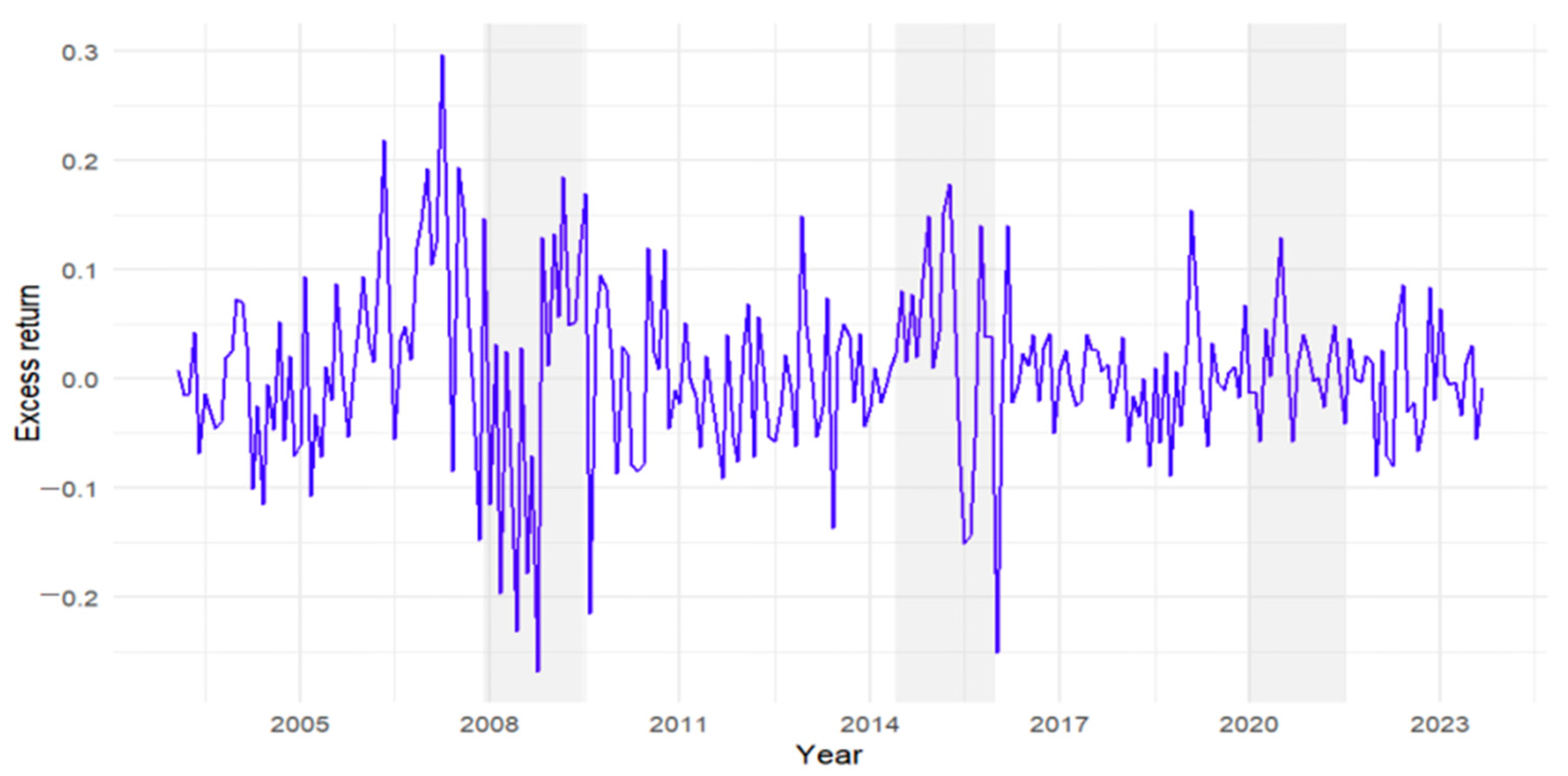
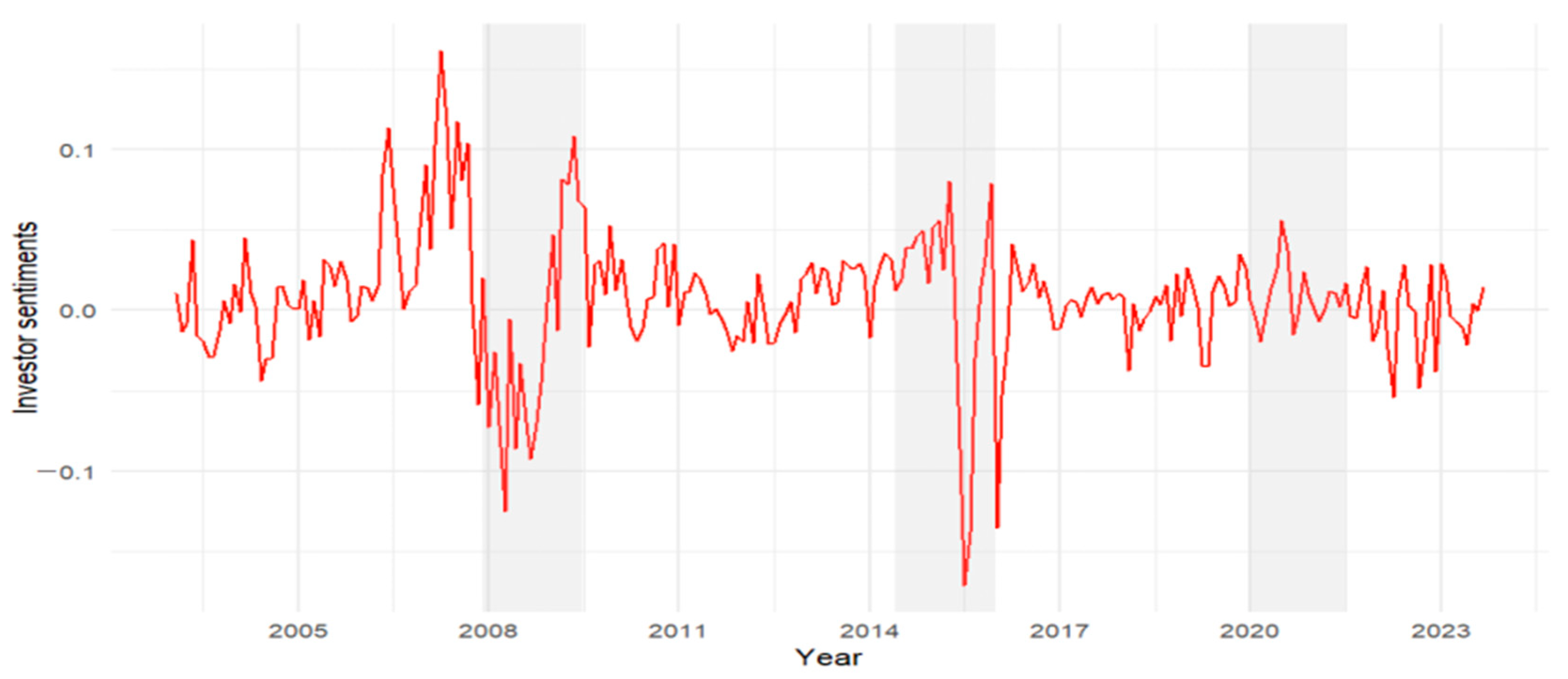
The predictability of investor sentiment has been shown to vary across different time periods [37]. Consequently, we perform the robustness check to evaluate whether the principal findings maintain statistical and economic significance in varying periods. The global financial market experienced a significant shock in 2008, known as the subprime mortgage crisis. The full sample is divided at the onset in December 2007. Similarly, the 2015 to 2016 Chinese stock market turbulence had a profound impact on investor confidence in future market conditions.

We run the regression model in Section 4.1 for S^PCA, S^PLS, S^GA, and S^GAN again over the four time periods. The temporal analysis employs systematically segmented intervals to evaluate sentiment predictability under distinct market regimes. For the 2008 financial crisis, the sample is stratified into pre-crisis (February 2003–December 2007) and post-crisis (January 2008–September 2023) phases. Similarly, China’s 2015 equity market correction is analyzed through pre-turbulence (February 2003–June 2015) and post-turbulence (July 2015–September 2023) windows. Table 9 presents the comparative predictive efficacy of sentiment metrics across these temporally stratified intervals, revealing structural variations in forecasting capacity during crisis versus noncrisis market states.

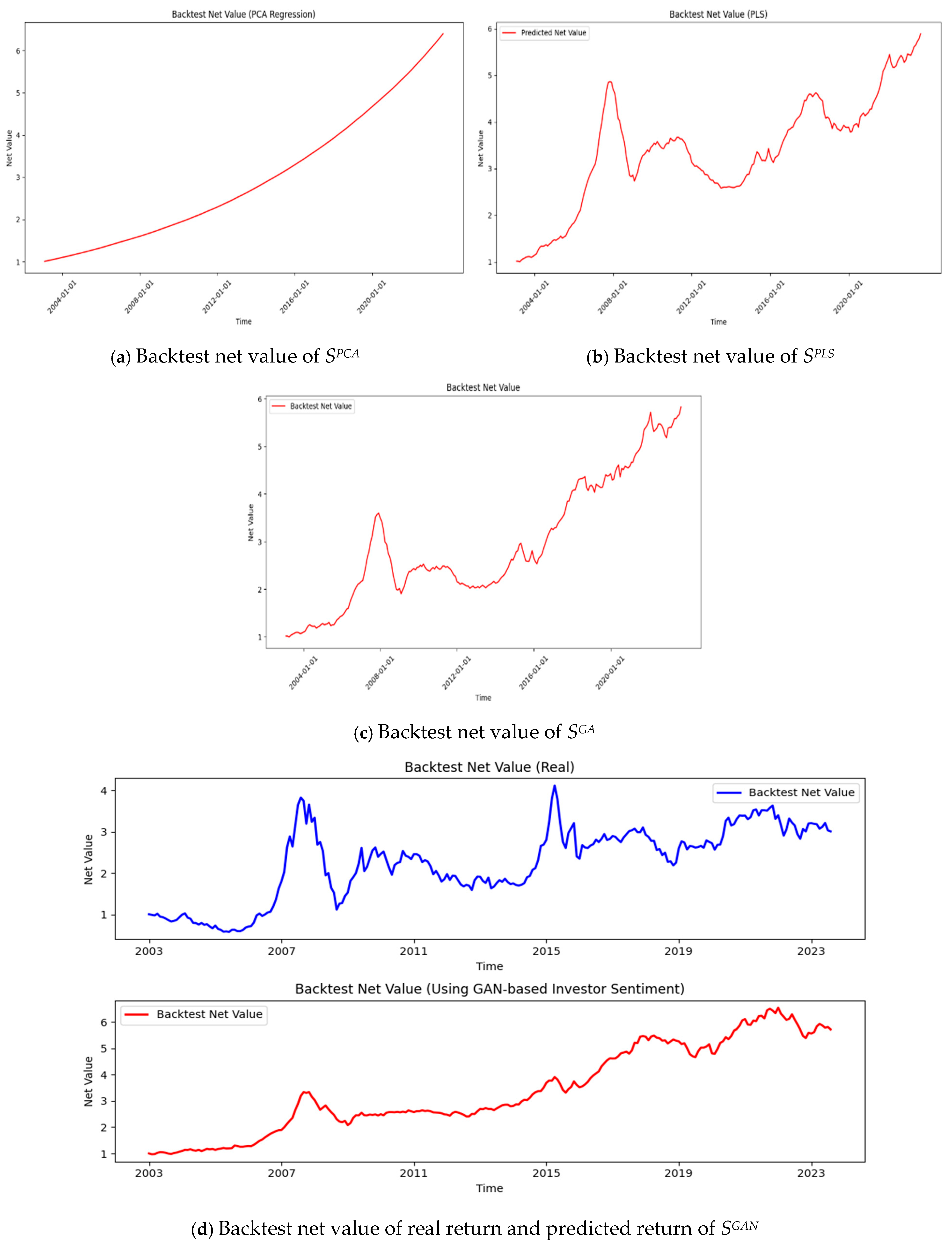
Table 10. Predictability before and after the financial crisis.

Predictor	Coefficient	t-Statistics	R2 (%)
Before the sub-prime crisis
SPCA	0.034	0.511	−7.9
SPLS	0.020 **	3.274	16.1
SGA	1.000 ***	4.077	22.6
SGAN	0.316 ***	8.090	28.4
After the sub-prime crisis
SPCA	0.032	0.498	−7.8
SPLS	−0.019 ***	−4.271	8.9
SGA	1.000 ***	6.161	16.9
SGAN	0.239 ***	14.932	19.7
Before China’s 2015 equity market correction
SPCA	0.029	0.612	−8.0
SPLS	0.028 ***	4.823	13.7
SGA	1.000 ***	5.949	19.4
SGAN	0.352 ***	9.366	22.5
After China’s 2015 equity market correction
SPCA	0.030	0.488	−8.1
SPLS	−0.018 ***	−5.191	21.9
SGA	1.000 ***	6.195	28.4
SGAN	0.196 ***	10.879	30.3

(Notes: This table reports robustness check results and predictivity results for the regression model in Section 4.1. For the 2008 financial crisis, the sample is stratified into pre-crisis (February 2003–December 2007) and post-crisis (January 2008–September 2023) phases. Similarly, China’s 2015 equity market correction is analyzed through pre-turbulence (February 2003–June 2015) and post-turbulence (July 2015–September 2023) windows. The specific indicators include coefficient, t-statistics, and R². Statistical significance levels are denoted by asterisks: ** at 5%, and *** at the 1% significance level).

provides a comparative analysis of different predictors. For example, before the subprime crisis, S^PLS exhibited significant positive predictive power, but after the crisis, its predictive ability turned negative, and its explanatory power decreased substantially, indicating that the market’s reliance on this variable weakened in the face of the crisis. S^GAN reflects the dramatic shift in market mood, showing a sharp drop in sentiment that corresponded with the market’s steep decline. The recovery seen later is captured by the rebound in sentiment, demonstrating S^GAN’s ability to predict the market’s reaction to global financial events and policy interventions.

A similar pattern is observed in the period surrounding the Chinese stock market turbulence. S^GAN exhibited greater robustness, as its predictive ability remained stable and even improved after the turbulence, with a significant increase in explanatory power. These results indicate that S^GAN demonstrates a high degree of robustness during both crises, effectively responding to external shocks, whereas S^PLS and S^GA show greater variability in their predictive performances across different stages.

5.2.2. Predictability During Bull Market, Bear Markets, and Turning Points

As a measure of market sentiment, the indicator exhibits strong indicative power in bull–bear market transitions. Specifically:

(1)

Bull Market: At the early stage of a bull market, S^GAN exhibits a gradual upward trend, indicating a steady improvement in investor sentiment. As the market reaches its late phase, S^GAN experiences a sharp surge, suggesting potential overheating and speculative bubbles.

(2)

Bear Market: In the initial phase of a bear market, S^GAN declines rapidly, reflecting a significant deterioration in investor confidence. Towards the end of the bear cycle, S^GAN remains at a low level but gradually recovers as signs of market stabilization emerge. A notable example is the 2008 global financial crisis, where S^GAN plummeted to a trough before gradually rebounding with the onset of economic recovery in 2009.

(3)

Turning Points: S^GAN tends to lead market return fluctuations at critical turning points, meaning that when it reaches an extreme high or low, a market trend reversal often follows. This characteristic makes S^GAN a valuable reference for investment strategies. For instance, a downturn from a high S^GAN level may signal rising market risks, prompting a more cautious approach, whereas an upward shift from a low S^GAN level may indicate a favorable entry point for investors.

5.2.3. Predictability During Bear Markets

In the Chinese stock market, bear markets are usually triggered by a range of economic, political, and market factors [36]. In the past few years, the Chinese stock market has experienced several notable bear markets, particularly in 2015, 2018, and 2021 to 2023 [38]. Market behavior during these bear markets provides an important opportunity to test the validity of investor sentiment indicators [39].

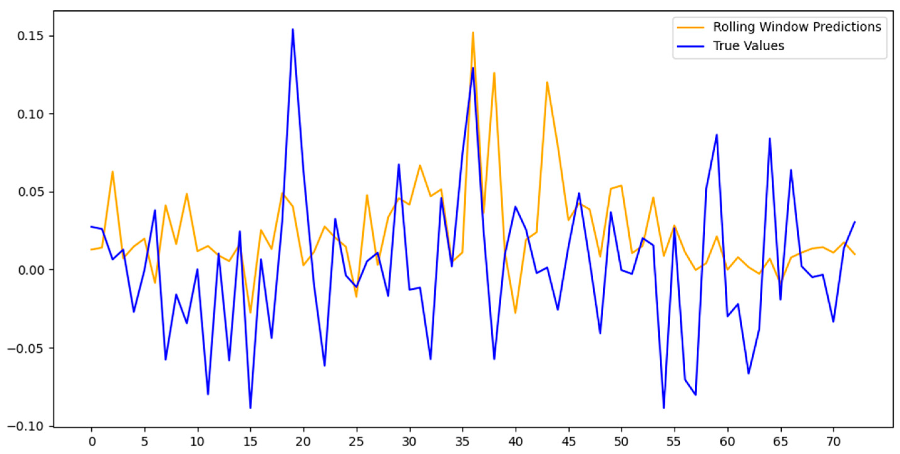
As can be seen in

Table 11. Predictability during bear markets.

Predictor	Coefficient	t-Statistics	R2 (%)
June 2015 to February 2016
SPCA	0.028	0.488	0.8
SPLS	−0.071 *	−3.696	61.3
SGA	1.000 ***	13.339	65.2
SGAN	0.589 ***	19.353	68.4
January 2018 to December 2018
SPCA	0.031	0.546	0.8
SPLS	−0.026 ***	−4.678	67.6
SGA	1.000 ***	12.479	70.4
SGAN	0.320 ***	9.496	71.8
January 2021 to September 2023
SPCA	0.030	0.522	0.8
SPLS	−0.025 ***	−4.325	36.4
SGA	1.000 ***	5.083	43.7
SGAN	0.256 ***	6.625	47.2

(Notes: This table reports robustness check results and predictivity results for the regression model in Section 4.1. The time periods include June 2015 to February 2016, January 2018 to December 2018, and January 2021 to September 2023. The specific indicators include coefficient, t-statistics, and R². Statistical significance levels are denoted by asterisks: * indicates significance at the 10% threshold, and *** at the 1% significance level).

, S^GAN has demonstrated strong forecasting ability during different bear market periods. During the crash between June 2015 and February 2016, the predictive performance of S^GAN is impressive and significant, with an R² of 68.4%, demonstrating the model’s high ability to explain excess market returns. In contrast, S^PCA has no predictive power in almost all the time periods. S^PLS performs relatively weakly, especially during the same period, with an R² of 61.3% and a negative coefficient, suggesting that its forecasts are not as good during this period. The performance of S^GA is relatively robust, with the significant coefficient and high R², but still not as good as that of S^GAN. In addition, during the other periods of the bear market, in 2018 and from 2021 to 2023, S^GAN still maintains a high R² value of 71.8% and 47.2%, respectively, showing its robustness and consistency across market cycles. Overall, S^GAN performs well in all bear market periods analyzed, proving its strong predictive ability as a sentiment indicator in extreme market conditions.

5.2.4. Which Market Behaviors (e.g., Speculation, Market Bubbles) Influence S^GAN Dynamics?

As an investor sentiment index, S^GAN captures various behavioral patterns in financial markets. It demonstrates notable sensitivity to specific market conditions, particularly in the following scenarios:

(1)

Speculation: Empirical evidence suggests that one of S^GAN’s key sentiment factors is market trading activity (TURN), which tends to increase during periods of heightened speculative behavior. For instance, in bullish markets, retail investors typically engage in higher trading volumes, leading to a surge in overall market sentiment, which is subsequently reflected in S^GAN’s upward movement.

(2)

Market Bubbles: S^GAN is also effective in identifying market bubble formations. During major bull runs, such as those in 2007 and 2015 of the Chinese A-share market, S^GAN recorded significant increases, signaling extreme investor optimism. Notably, before a bubble bursts, S^GAN often exhibits an early downward trend.

(3)

Flight to safety: During periods of heightened market uncertainty, such as the 2008 global financial crisis and the 2020 COVID-19 pandemic, S^GAN experienced a pronounced decline, reflecting deteriorating investor sentiment and a shift towards safer assets. This trend aligns with the movement of the VIX index (volatility index), reinforcing S^GAN’s ability to capture risk aversion behavior under financial distress.

5.2.5. How Do S^GAN’s Core Sentiment Factors Relate to Investor Behavior?

The key sentiment factors extracted by S^GAN using deep learning techniques exhibit strong associations with investor behavior in financial markets. These relationships are particularly evident in the following aspects:

(1)

Market Participation:

①

Key Factors: TURN (trading volume), NIA (number of new accounts).

②

Trading volume and the number of newly opened accounts serve as indicators of investor enthusiasm. When market sentiment strengthens, these metrics tend to rise, and S^GAN correspondingly reflects this upward trend.

(2)

Speculative Trading

①

Key Factors: IPOR (IPO first-day return), IPON (number of IPOs).

②

A heightened preference for high-risk assets is often accompanied by an increase in IPO first-day returns and the number of IPOs. S^GAN captures this dynamic, signaling periods of intensified speculative activity.

(3)

Market Uncertainty

①

Key Factor: EPU (economic policy uncertainty index).

②

During times of rising uncertainty—such as policy shifts or geopolitical tensions—investor sentiment tends to weaken. This is reflected in a decline in S^GAN, indicating a more cautious market outlook.

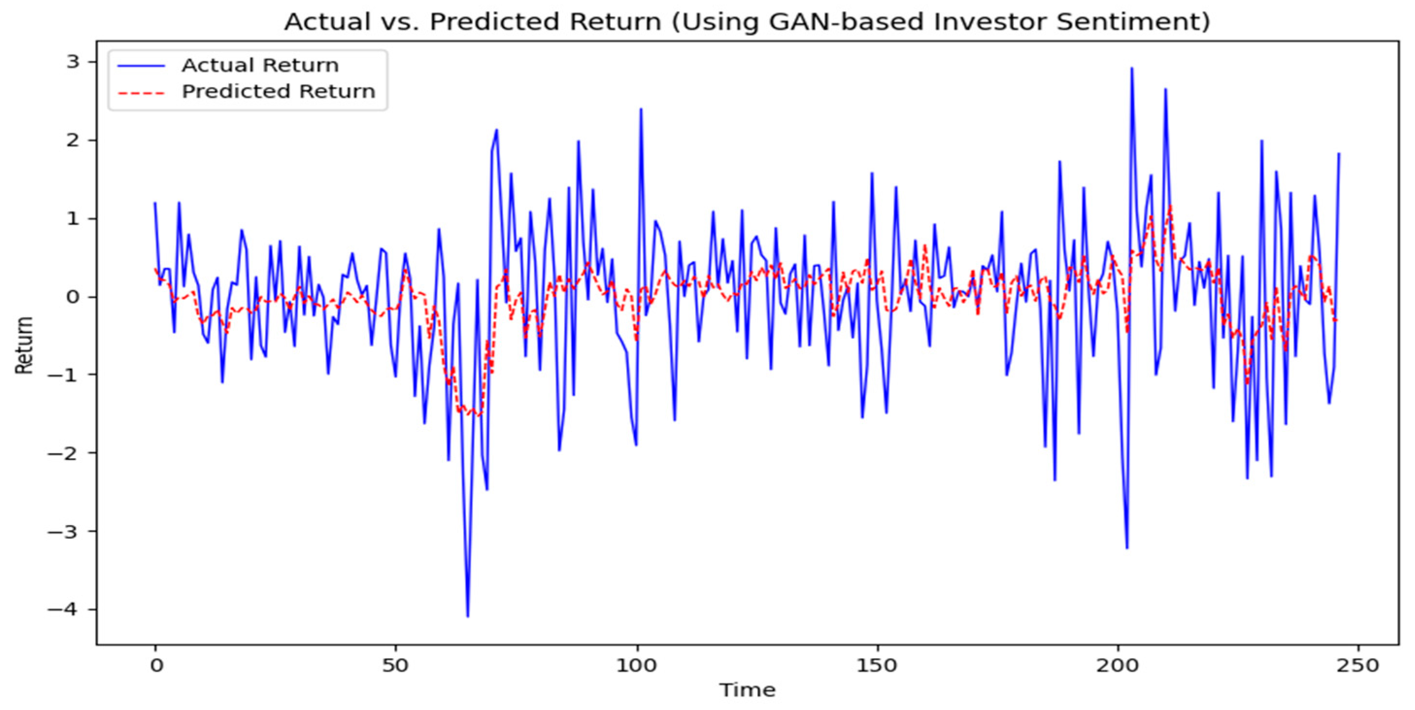
5.3. Predictability of S^GAN in the American Stock Market

In order to briefly examine the dimensionality reduction effect of the GANs on various investor sentiment proxies in different market environments, we selected the five most representative sentiment proxies in the U.S. stock market for dimensionality reduction analysis. These five indicators are dividend premium (PDND), closed-end fund discount (CEFD), number of IPOs (NIPO), first-day returns on IPOs (RIPO), and equity share in new issues (S). They are all from the New York University Stern School of Business, while excess market returns (R^m) data are from the Tuck School of Business at Dartmouth. The period selected for this test is from November 2003 to November 2023.

Based on the similar methodology in Section 4.1, our empirical analysis shows that investor sentiment has a significant positive impact on stock market returns. Figure 13 compares the predicted returns with actual returns. As can be seen from the figure, the overall trend of actual returns is closer to that of predicted returns, suggesting that the model has demonstrated some validity in capturing the overall direction and trend of market returns. In addition, the F-statistic of the regression analysis and its corresponding p-value indicate that the overall model is highly significant, which further validates that the downgraded sentiment proxies are still effective in capturing the dynamic relationship of market returns. Moreover, we use the Diebold–Mariano test to assess the statistically significant differences in the forecasting models. The results show that S^GAN has a significantly superior forecasting accuracy with the DM statistic of 2.87, and the p-value is less than 0.01. It confirms the robustness of our model’s predictive ability in different market environments. This formal statistical test provides an objective basis for this model. In other words, the investor sentiment extracted by the GAN method still represents excellent explanatory ability in the prediction of U.S. market returns.

5.4. Theoretical Basis and Mechanism Analysis of S^GAN’s Superiority

This section explores the intrinsic theoretical basis of the superiority of S^GAN over traditional methods. The results of the empirical analyses show that S^GAN significantly outperforms methods such as S^PCA, S^PLS, and S^GA in predicting the excess returns of China’s A-share market, and this superiority stems from the following key mechanisms.

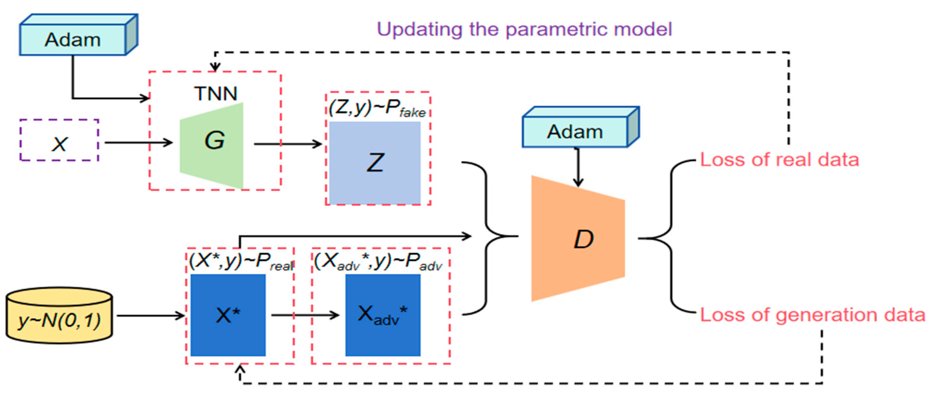
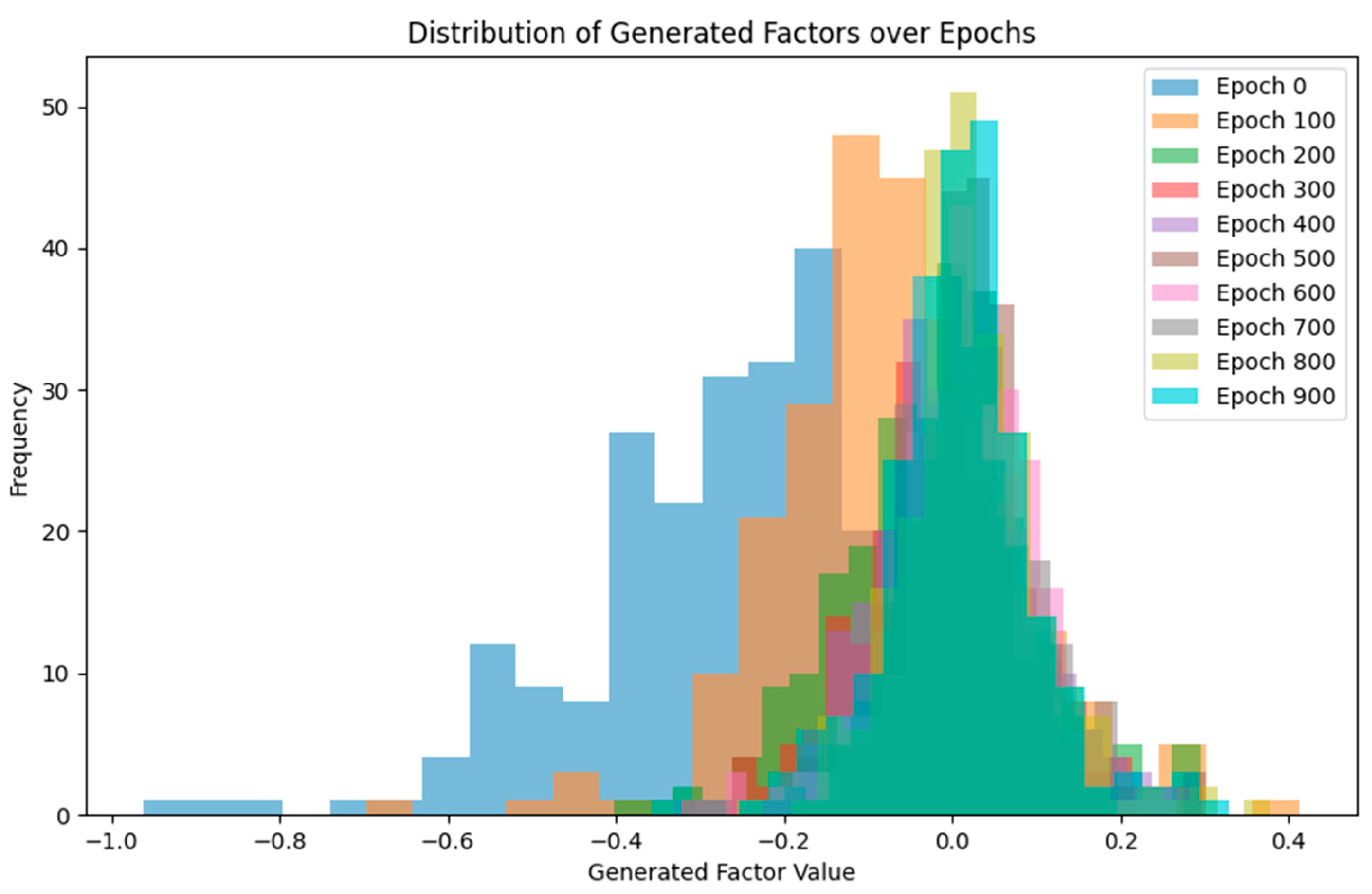
Firstly, the nonlinear feature extraction capability of GANs enables S^GAN to effectively capture the complex relationships among sentiment proxy variables. Financial markets are inherently nonlinear systems, and the relationship between investor sentiment and market behavior often exhibits complex nonlinear patterns. Traditional methods such as PCA and PLS are mainly based on linear assumptions, and it is difficult for them to capture this complexity. GANs, on the other hand, are able to automatically learn the nonlinear dependencies between sentiment agents through multilayer neural networks and adversarial training without the need to pre-specify the form of the parameters. The feature importance analysis in Figure 9 confirms the more complex and balanced emotional structure captured by S^GAN.

Secondly, the adversarial training mechanism provides powerful noise filtering capabilities. Financial market data typically contain a large amount of noise that may interfere with the extraction of sentiment signals. The discriminator of S^GAN effectively filters out extraneous noise by constantly challenging the generator and forcing it to extract the most informative sentiment factors. This mechanism is particularly important during periods of high market volatility, explaining why S^GAN performed stably during the 2008 financial crisis and the 2015 market turmoil.

Thirdly, S^GAN’s adaptive feature weight assignment mechanism makes it highly sensitive to changes in the market environment. Unlike the static weights used by S^PCA and S^PLS, S^GAN is able to dynamically adjust feature weights according to the market environment. This feature is particularly critical for capturing rapid changes in investor sentiment, such as at bull–bear transition points, where S^GAN can quickly adjust the weights of liquidity indicators such as TURN and RV to more accurately predict market turns. This explains why S^GAN significantly outperforms other indicators during bear markets, as shown in Table 10.

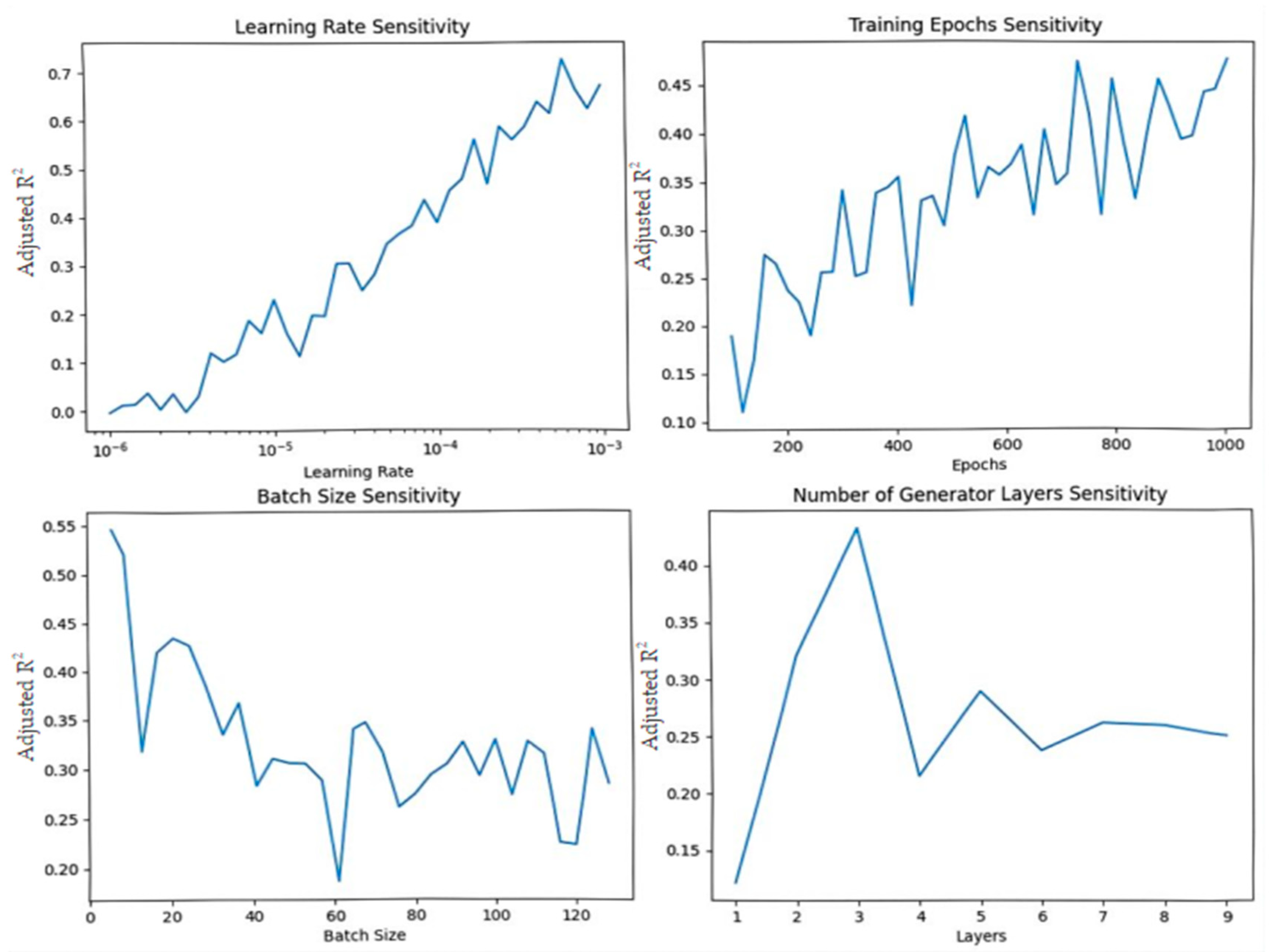
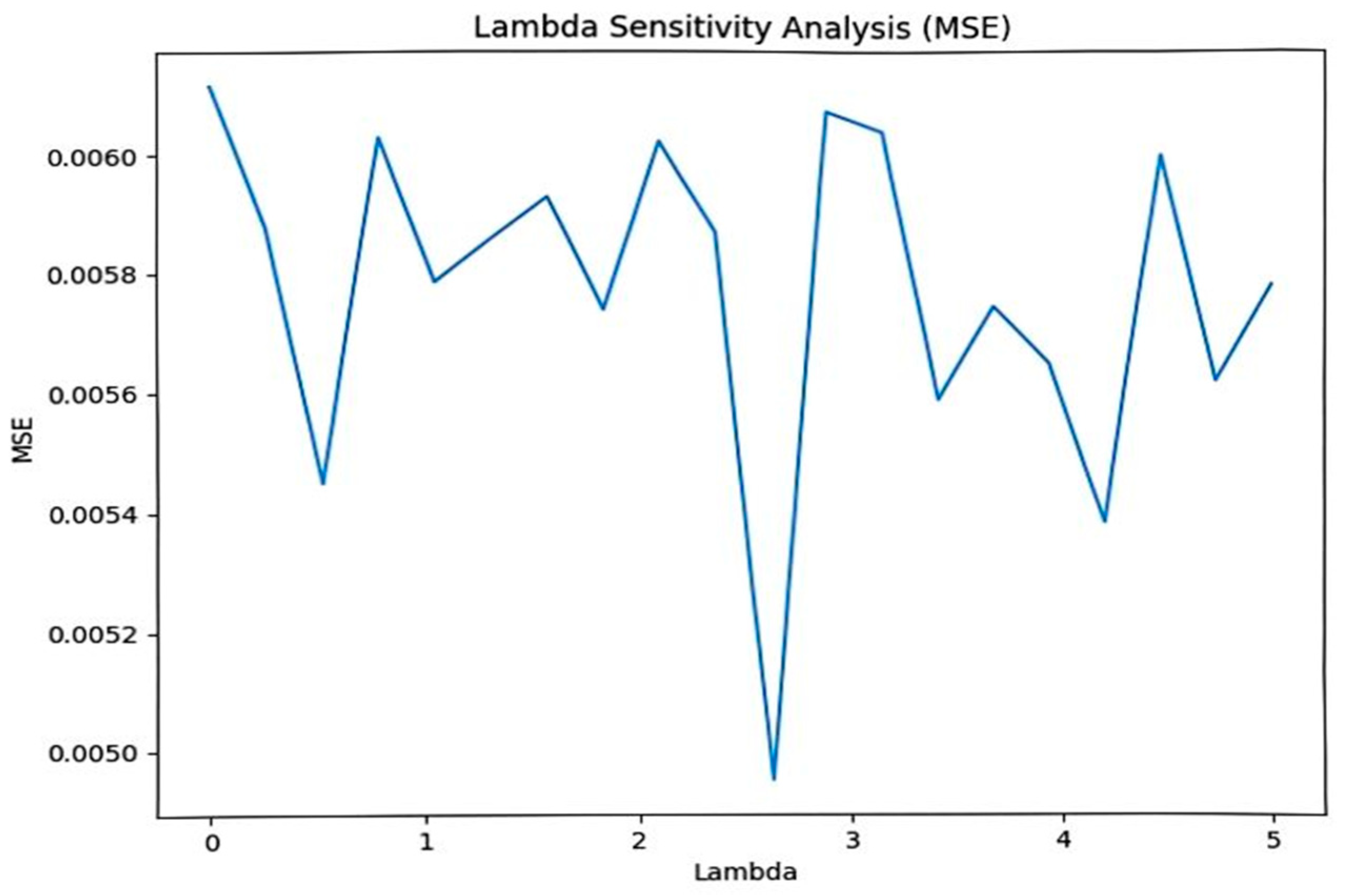
Finally, the integrated loss function we designed ensures that S^GAN maintains economic explanatory power while preserving statistical significance. The λ-sensitivity analysis in Figure 5 shows that this balance is critical to model performance. In addition, the model collapse prevention strategy we employ enhances the generalization ability of S^GAN to maintain stable performance under different market conditions.

In summary, the theoretical basis of S^GAN’s superiority lies in its ability to capture complex nonlinear sentiment structures, filter market noise, dynamically adapt to changes in market environments, and strike a balance between statistical significance and economic explanatory power through the unique architecture of GANs. These properties make S^GAN promising for a wide range of applications in asset pricing and market forecasting.

5.5. Computational Complexity and Limitations of Proposed Approach

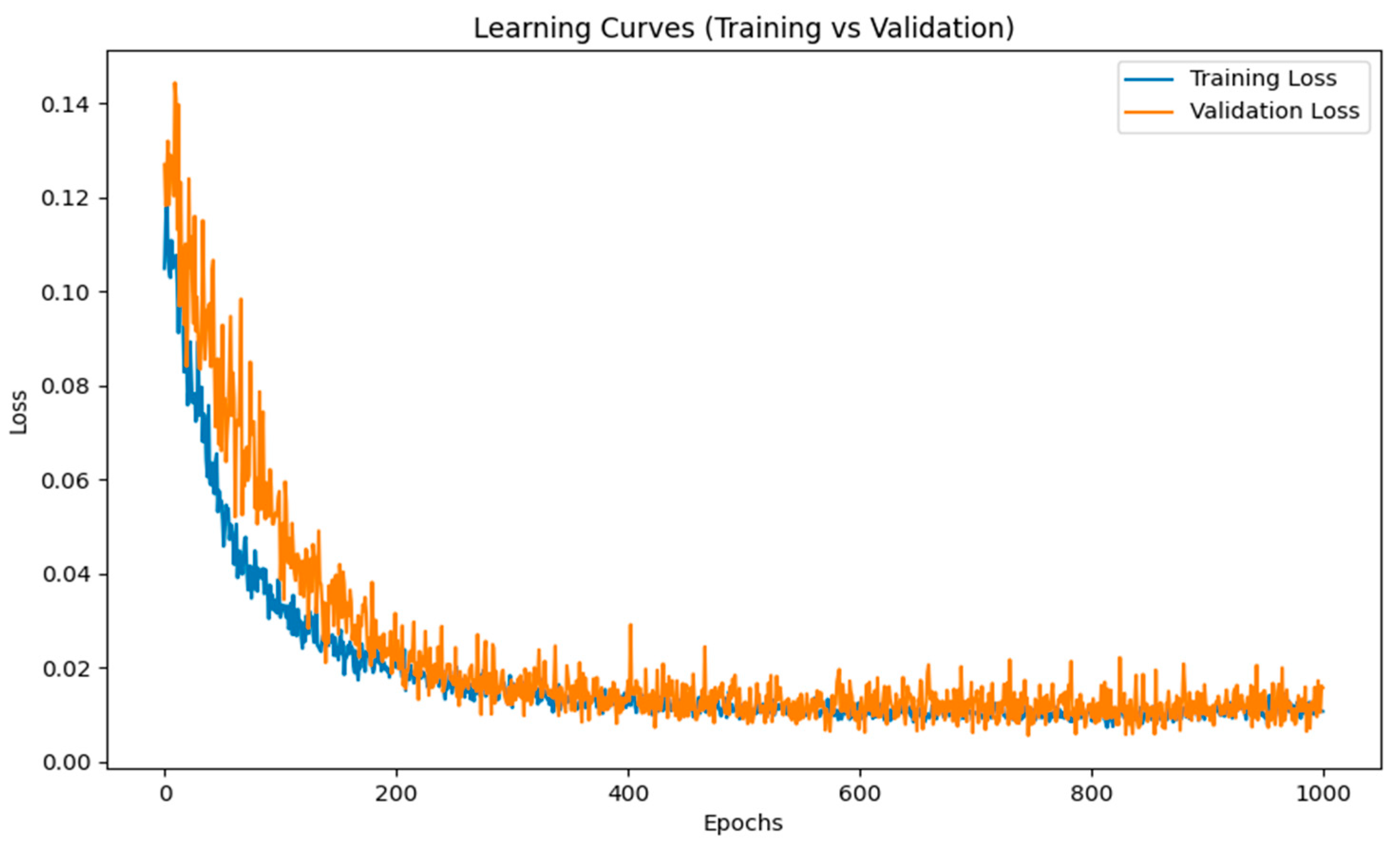
In this test, the GANs need to compute forward propagation and backpropagation once for both the generator and discriminator within each epoch. Assuming that the dimension of our input data is $d$, and we have trained $E$ epochs, the total computational complexity of each epoch is $o(E\ast n\ast (d+32))$, which is the computational complexity of each iteration in the training process. The total training time is 1.53 s. However, the GAN method in this experiment has some limitations. Firstly, the GANs in this study use a single potential dimension to represent investor sentiment. Nevertheless, financial market sentiment is complex, and multiple dimensions may be required to adequately describe investor mood swings and market psychology. If the potential dimension is too small, it may not capture all the useful sentiment signals; if it is too large, it may introduce noise or cause excessive model complexity. Second, for the agents that need to be downgraded in this study, we selected appropriate hyper-parameters to enable effective cooperation between the generator and the discriminator, so that better quality sentiment signals can be extracted. However, if this method is extended without improvement to deal with complex financial data problems, the gaming process between generators and discriminators may lead to unstable training, which makes the extracted correlation signals distorted. Meanwhile, GANs are highly prone to overfitting the training data when dealing with correlated data. Especially in financial data, the market data have strong time dependence and seasonal fluctuations, and overfitting may lead to an inconsistent performance of sentiment signals in different time periods. Finally, financial market sentiment is determined not only by factors such as historical prices and technical indicators, but is also influenced by external factors such as macroeconomics, policies, international events, and so on. The GAN model may not be able to adequately capture the impact of these factors on sentiment, resulting in the extracted sentiment signals failing to reflect the complete market psychology.

Regarding the applicability of S^GAN in different trading frequency scenarios, although this study’s analyses are mainly based on monthly data, the method has flexibility and limitations in practical application. For high-frequency trading environments, S^GAN faces two main challenges, which are computational latency and the high-frequency nature of emotional agents. The training process of GAN models is relatively time-consuming and is not suitable for real-time re-training in very high-frequency trading with millisecond decision requirements. However, the inference phase of the trained models is very efficient, which means that S^GAN can be useful in low- to medium-frequency trading strategies, such as intraday trading and daily or weekly investment decisions. Hybrid strategies can be used in practical applications: for example, the model can be updated weekly using the latest data, while the prediction process can take place in real time. In addition, high-frequency application scenarios require the redesign of sentiment proxies to suit short-term market volatility, which may be an important direction for future research. Overall, S^GAN is best suited for low- to medium-frequency trading strategies with daily to monthly time horizons and is able to effectively balance predictive performance and computational efficiency in these scenarios. For portfolio managers, S^GAN can be used as an asset allocation decision tool to enable countercyclical investment strategies; market analysts can use it as a leading indicator of market turnaround, which performs particularly well in extreme market environments; and financial economists can use it to delve into the nonlinear relationship between sentiment and asset pricing.

6. Conclusions

Investor sentiment, a key behavioral indicator in the stock market, was constructed using various methods in prior research. This study introduces a novel investor sentiment, S^GAN, developed using GANs. Leveraging GANs, we synthesized latent factors from eight sentiment indicators and assessed their predictive abilities for excess returns in the Chinese A-share market. The empirical results demonstrate that GAN-based investor sentiment outperforms traditional sentiment measures derived from PCA, PLS, and GA in both in-sample tests and out-of-sample tests. Meanwhile, S^GAN remains statistically significant even after controlling for macroeconomic variables, indicating that it captures market-relevant information beyond economic fundamentals. Additionally, S^GAN exhibits strong predictive power across various industries, with the financial sector showing the highest sensitivity to investor sentiment, aligning with prior research findings. Last but not least, its predictive ability remains robust across different economic periods and countries, further affirming its stability.

In summary, this study innovatively applies GANs to investor sentiment modeling, breaking through the limitations of traditional linear downscaling methods and providing a new research paradigm for financial behavior. The unique ability of GANs to capture the nonlinear features of sentiment time series provides a new perspective to understand how market sentiment drives price fluctuations, and this methodological innovation not only improves the prediction accuracy, but also provides a theoretical basis for constructing more effective investment strategies. Moreover, we find that the lagged effects and asymmetric responses of sentiment indicators play a crucial part in the performance of GAN models. GANs are able to capture these lagged sentiment fluctuations efficiently through adversarial training to improve the predictive power of sentiment indicators, and at the same time deal with such asymmetric effects efficiently, so that the sentiment indicators can accurately reflect the way the market responds to different changes in sentiment. This enables GANs to outperform traditional approaches to sentiment analysis, providing more stable and predictive sentiment signals across a wide range of economic conditions, thereby improving the accuracy of the predictions of future market returns. Future research could be directed toward a comprehensive empirical investigation to select additional sentiment proxies and apply a GAN to develop more robust investor sentiment indicators. Additionally, it is of interest to adopt increasingly advanced dimensionality reduction methods to explore a broader range of stock markets.