1. Introduction
The foreign exchange market (forex or FX) is a global marketplace where currencies are traded. It is the world’s largest market, averaging USD 6.6 trillion in daily trading volume [
1]. The vast, decentralized forex market enables various participants, from central banks to individual investors, to capitalize on currency fluctuations driven by global economic factors, political events, and market sentiment [
2]. As a result, the forex market is a dynamic interplay of supply, demand, and global events, constantly influencing currency prices. The forex market operates 24/5, excluding weekends and bank holidays. Currencies are traded in pairs, allowing traders to profit either by buying low and selling high or by short-selling (selling borrowed currency and buying it back at a lower price). However, forex trading is highly speculative and carries significant risk. Traders use fundamental and technical indicators to forecast future currency prices. Fundamental analysis assesses a currency pair’s intrinsic value based on economic factors such as GDP, inflation, interest rates, and unemployment, while technical analysis employs mathematical calculations on historical price data, including trends, momentum, volatility, and volume indicators. More details on these indicators are provided in
Section 3.
The EUR/USD pair, accounting for 22.7% of global forex trades in 2022, a slight decrease from 24% in 2019 [
1], is a popular subject of research due to its significant market impact. While deep learning offers promising results in forex forecasting, predicting closing prices is challenging due to factors such as multi-factor influence, high volatility, market efficiency, non-stationarity, noise, interconnected markets, and regulatory impacts [
3,
4]. Addressing these complexities requires specialized models and techniques that leverage advanced statistical models, machine learning, and external data sources to improve prediction accuracy.
In this work, we propose a dual-input deep-learning model that takes a wide range of fundamental and technical indicators as inputs and forecasts the closing price of EUR/USD with high probability. While the effects of each type of indicator/data are initially input separately into the network, they are eventually integrated to enhance the outcome of the proposed predictive model. To this end, a dual-input deep-learning long short-term memory (LSTM) model,
-
, as first introduced by Hochreiter and Schmidhuber [
5], is proposed to forecast the future EUR/USD closing price. The proposed model accepts various fundamental and technical indicators as inputs to improve forecast accuracy without requiring EUR/USD closing prices as input, which gives it an advantage over alternative models in the literature.
The proposed model is tested against alternatives, and its superior performance is verified. Moreover, forecasts for the next three days are obtained. Additionally, in a sensitivity analysis, forecasts are provided under various scenarios concerning the values of fundamental indicators.
The rest of the manuscript is organized as follows. An overview of the most recent and pertinent research is presented in
Section 2. The materials used in this article are detailed in
Section 3. The proposed method is formulated and outlined in
Section 4, and results, along with comparisons, are reported in
Section 5. Finally, concluding remarks and discussion are provided in
Section 6.
2. Related Work
Recent studies have explored the use of deep learning, particularly LSTM neural networks, for forecasting FX volatility. While these approaches have advanced the field by improving time-series modeling, they often rely on single-input architectures or treat technical and fundamental indicators in isolation. In contrast, this study introduces a dual-input LSTM-based architecture that explicitly integrates both technical and fundamental indicators in parallel streams, allowing for more nuanced learning of market dynamics. Additionally, the model leverages carefully selected time frames and normalization strategies to further enhance prediction accuracy. The following review situates this work within the broader literature, with a focus on model architecture, indicator selection, and time-series handling in similar deep learning-based financial forecasting efforts.
Initially, Dautel et al. [
6] investigated the potential of deep learning, specifically LSTM and GRU networks, for exchange rate forecasting. Their findings suggest that these modern architectures outperform traditional RNNs [
7] in terms of forecasting accuracy, highlighting the value of deep learning in this domain. In the study of time-series, convolutional neural networks (CNNs) represent another deep neural network class that can automatically extract features and create informative representations of temporal data. The effectiveness of CNNs in forecasting time-series was first discussed by Markova [
8]; while CNNs can extract features from temporal data, they may not capture long-term relationships as effectively as RNNs. To address this, multivariate multi-step CNNs and hybrid approaches combining CNNs and RNNs have been proposed (see Ni et al. [
9], Sako et al. [
10] for a few examples). While hybrid CNN–RNN models focus on extracting both short- and long-term features, our architecture emphasizes the integration of diverse feature types, both technical and fundamental, within a unified recurrent structure. Sako et al. [
10] provide a comparative analysis of LSTM and GRU networks for forecasting stock market indices and currency exchange rates. Additionally, Jung and Choi [
11] proposed a hybrid LSTM–autoencoder model [
12] to capture complex and dynamic input sequences. This model leverages the memory cells of LSTM layers in both the encoder and decoder components to learn long-term dependencies in the data, implemented using deep learning API tools.
The choice of time frame is crucial in forex prediction. Longer time frames, like monthly intervals, offer more stable patterns, while shorter time frames, such as minutes, are more volatile. It is common for different time frames to show contradictory patterns [
13]. While Dobrovolný et al. [
14] explored time frame effects on LSTM-based EUR/USD price prediction, challenges like network architecture, window size sensitivity, and variable scaling remain. Unlike [
14], which focuses on time frame sensitivity in univariate LSTM models, our approach extends this by assessing time frame interactions within a dual-input, multivariate framework.
Authors Kaushik and Giri [
15] and Kamruzzaman and Sarker [
16] have shown that multivariate time-series models, which incorporate multiple relevant features such as technical, fundamental, and inter-market indicators, can improve forex prediction accuracy. Munkhdalai et al. [
17] further advanced this approach by introducing a locally adaptive, interpretable deep-learning architecture augmented with RNNs to capture the dynamics of input and output variables.
The choice of indicators, both technical (e.g., MA, MACD, and RSI) and fundamental (economic statistics), is critical for forex prediction. These indicators can be combined for joint analysis or used separately. Yıldırım et al. [
18] employed different LSTMs for technical and fundamental indicators, combining their outputs through smart decision logic. Prediction outcomes can be treated as binary classification (decrease/increase) or three-class classification (decrease/no change/increase), as seen in [
6] and Yıldırım et al. [
18], respectively.
Unlike our proposed dual-input architecture, which processes technical and fundamental indicators simultaneously in parallel streams, [
18] trained separate LSTM models and combining their outputs post hoc via decision logic.
Table 1 and
Table 2 summarize general machine learning approaches used to forecast forex values, including both shallow-learning and deep learning-based models.
Table 3 provides an overview of various methods commonly used in finance and forex forecasting applications, categorized by prediction, portfolio management, risk assessment, and pattern recognition.
In summary, while prior studies have demonstrated the effectiveness of LSTM-based models in exchange rate forecasting, they typically rely on either single-stream architectures or limited sets of features. This study contributes to the literature by introducing a dual-input LSTM architecture that jointly processes technical and fundamental indicators optimized for both short- and long-term pattern recognition. This methodological design, alongside a systematic exploration of time frame and normalization strategies, offers a more integrated and potentially more accurate approach to forex prediction.
3. Materials
The daily high, low, and closing prices for the EUR/USD exchange rate were acquired from 3 January 2000 to 14 March 2025, totaling 6575 daily values [
38]. For the same time period, the daily U.S. long-term interest rate was collected as a fundamental indicator [
39]. Other fundamental indicators, including the EUR inflation rate [
40], U.S. inflation rate [
41], EUR long-term interest rate [
42], EUR unemployment rate [
40], and U.S. unemployment rate [
43], are monthly rates obtained separately from reliable online sources. These monthly rates were then duplicated to fill in daily values.
Six technical indicators were generated using the daily EUR/USD exchange rates via Python 3.11.0’s ‘ta’ library [
44]. These indicators are the exponential moving average (
), moving average convergence/divergence (MACD), relative strength index (RSI), upper and lower Bollinger bands (BBs), and average true range (
).
Table 4 provides the formulas for these indicators. Note that the MACD uses a simple moving average (
) with a window size of 26. As a result, no MACD value is calculated for the first 25 observations, so these are excluded, leaving 6550 observations for further analysis, starting from 7 February 2000. Additionally, an
of 6 is applied to the RSI and
values to smooth sharp fluctuations in these indicators. Time plots of all utilized fundamental and technical indicators are provided in
Supplementary Material Figures S1 and S2.
No volume indicators were utilized because not all brokerage firms publish trade volume in a standardized format, making reliable daily volume data inaccessible. All computations in this article were performed using Python 3.8.5 with the TensorFlow 2 package on a Windows OS 10 with a Core i7-10750H CPU and 32 GB RAM. All data and code are available to researchers at
https://github.com/asaghafi/Forex, accessed on 28 April 2025.
4. Methods
Figure 1 outlines the proposed model. The steps are as follows:
4.1. Pre-Processing
The six fundamental and six technical predictors are stored in a
2D array, while the closing prices are stored separately in a vector of length 6550. To assess the model’s performance,
of the most recent data is designated as the test set. The remaining
is split into a
training set and a
validation set. The array of predictors and the response vector are then processed with a robust scaler, where each predictor is centered by subtracting its median and scaled by its inter-quartile range as follows:
This approach scales features using statistics that are less sensitive to outliers. Next, the scaled predictors and response are processed with a min–max scaler:
The scaler functions are calculated using the combined training and validation data.
There is evidence supporting performance improvements in many machine learning algorithms when data are properly scaled [
45,
46]. Using
training data and
validation data, we conducted a comparative study with 10 runs of the dual-input model, each initialized with different random seeds, under four conditions: with or without the robust scaler and with or without the
scaler. The median and quartiles for scaling were calculated using only the training data. All model hyperparameters were set as described in the model structure.
Table 5 summarizes the comparison results.
Results indicate that, on average, using both scalers achieves lower minimum and values in both the training and test sets. Additionally, the variability in these performance metrics is reduced. These statistics are calculated before transforming the data back to their original scale. We also calculate the overall training + validation and after transforming the data back to their original scale, further demonstrating the performance improvement when both scalers are applied. Notably, instances of non-convergence in network weights, where the model failed to generate accurate predictions, were more frequent when the robust scaler was not used.
While we did not attempt to make the input and output variables stationary, this is a common practice in many deep learning models [
47,
48]. However, it is important to recognize that deep learning models for time-series data do not require stationary assumptions, and there are many successful implementations without this requirement [
49,
50].
Following a
training,
validation, and
test split, the validation data were used to develop the model structure and to estimate hyperparameters, including the number and type of layers, layer parameters, number of training epochs, loss function, and scaling effectiveness, among other considerations. The structure of the finalized model is illustrated in
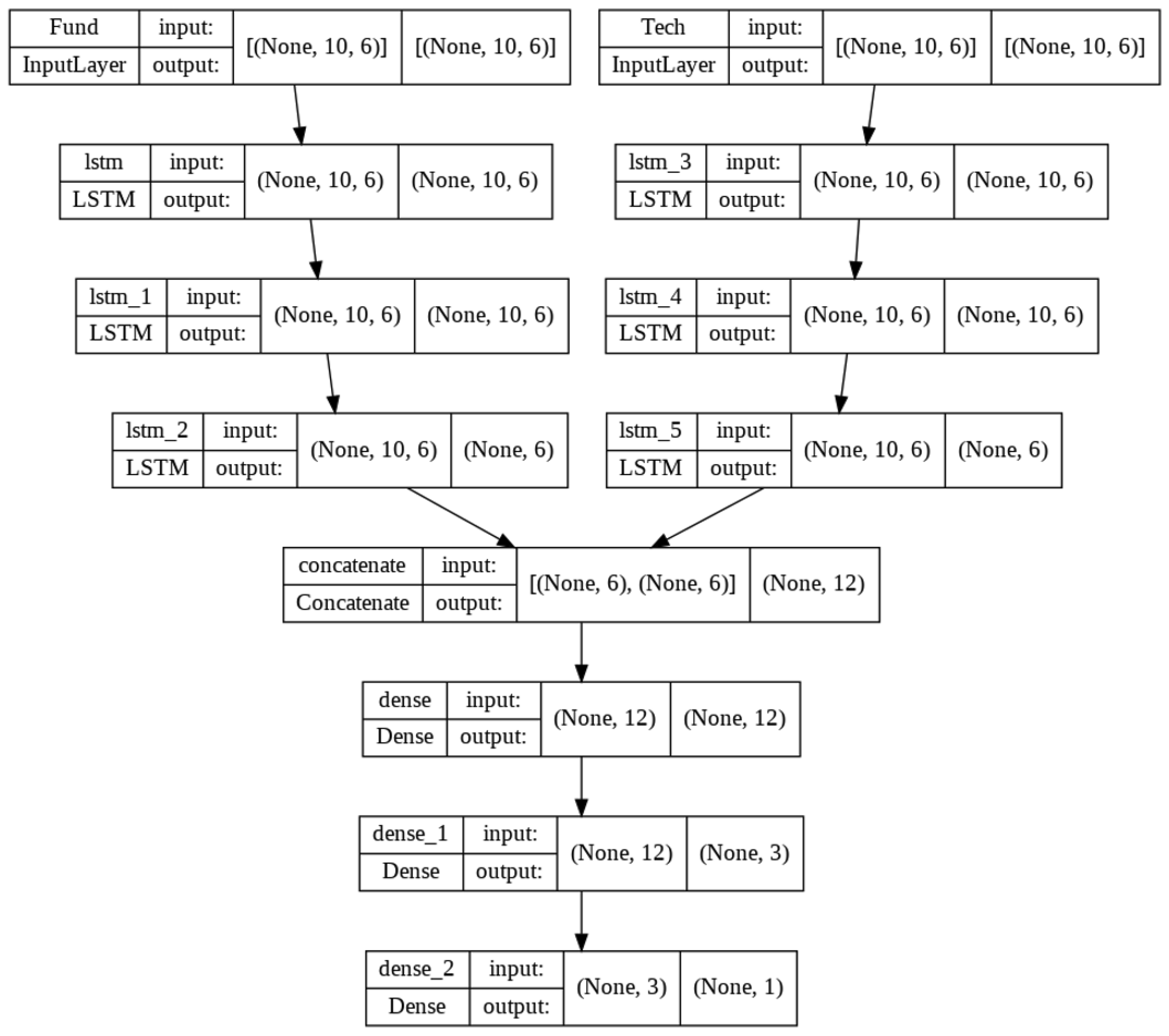
Figure 2.
This model consists of five hidden layers: . The layers are described as follows:
Input: Fundamental and technical indicators are stored in two separate 2D arrays of size . These are fed into the dual-input network in batches.
LSTM: Three LSTM layers, each with six units, are applied on each side of the dual-input network, where they process information forward and retain the long-term memory of sequences.
Concatenate: The output from the last LSTM layer on the fundamental side is concatenated with the output from the technical side, forming 2D arrays.
Dense: Two fully connected dense layers with 12 and 3 neurons, respectively, are used. Each neuron connects to all neurons in the previous layer, with the ReLU activation function applied to both layers.
Output: A fully connected dense layer with one neuron and a linear activation function serves as the final output layer.
After finalizing the model structure, the validation data are added to the training data. The model is then trained 100 times with different random seeds, and the memory and weights are cleared between each run. The weights and performance metrics for each model run are stored for post-processing. The training hyperparameters that were selected through the validation process include the ‘Adam’ optimizer, ‘MAE’ metric, 600 epochs, a batch size of 64, and the ‘Huber’ loss function, defined by the following:
The Huber loss applies a quadratic penalty for small errors and a linear penalty for large errors [
51]. By default,
is determined automatically.
4.2. Post-Processing
Model performance is evaluated on the training, validation (used only for hyperparameter tuning), and test sets using the root mean squared error (
) and mean absolute error (
) of closing prices and their model predictions.
, a widely used performance metric for regression problems, is defined as follows:
where
T is the number of time instances,
is the observed closing price at time
t, and
is its prediction by the model.
values are non-negative, with lower values indicating better model performance.
, another popular non-negative performance metric, penalizes errors linearly and is defined by the following:
Like , lower values indicate better model accuracy. A threshold of is applied to in both the training and test sets to filter out models with suboptimal performance among the 100 trained models.
4.3. Forecasting
To forecast the next-day closing price, the selected best models are retrained for 300 epochs using the extra test data. The final best models that achieved less than 0.008 are used to generate next-day forecasts. The forecasts are then transformed back to their original scale. A boxplot of forecasts is plotted using the final best models, demonstrating the variability of the next-day forecasts. The forecasted high, low, and median prices are then stored and passed on to the next step to facilitate further forecasts.
4.4. Re-Pre-Processing
The next-day forecasted high, low, and closing prices are re-scaled using inverse transformation methods. These values are then added to the original dataset as the last instance, while the first instance of the data is removed. Using this updated dataset, technical indicators are recalculated. Next-day forecasts for fundamental indicators are also obtained and appended to the data. The updated dataset is then passed to the forecasting step for retraining with the additional test data, generating the subsequent day’s forecast. This process is repeated to produce forecasts for the following three days.
5. Results
To evaluate performance, the proposed dual-input LSTM model was compared with three related models: F-LSTM (using only fundamental indicators), T-LSTM (using only technical indicators), and FT-LSTM (using both types of indicators as a single input to an LSTM). Due to differences in model complexity, training was conducted over varying epochs: 300 epochs for F-LSTM and T-LSTM, 600 for the dual-input LSTM, and 900 for FT-LSTM, with epoch counts roughly proportional to each model’s parameter count. All other hyperparameters were kept constant. Following 100 training runs,
and
metrics were computed for the both training and test sets, as summarized in
Table 6.
Given the parameter count and average training time, the dual-input model shows a balanced architecture. It achieves an average test of over 100 runs. For F-LSTM, T-LSTM, and FT-LSTM, the average test values are , , and , respectively. On average, the dual-input model surpasses the other models in predictive accuracy on the test set. While T-LSTM performs slightly better than the dual-input model on median test values, the dual-input model outperforms all alternatives in train , indicating it is more effectively trainable. This advantage is even clearer when comparing values.
The average test across 100 runs for the dual-input, T-LSTM, FT-LSTM, and F-LSTM models is , , , and , respectively, underscoring the superior performance of the dual-input model. The other models produce larger errors, significantly impacting their but not affecting their as much.
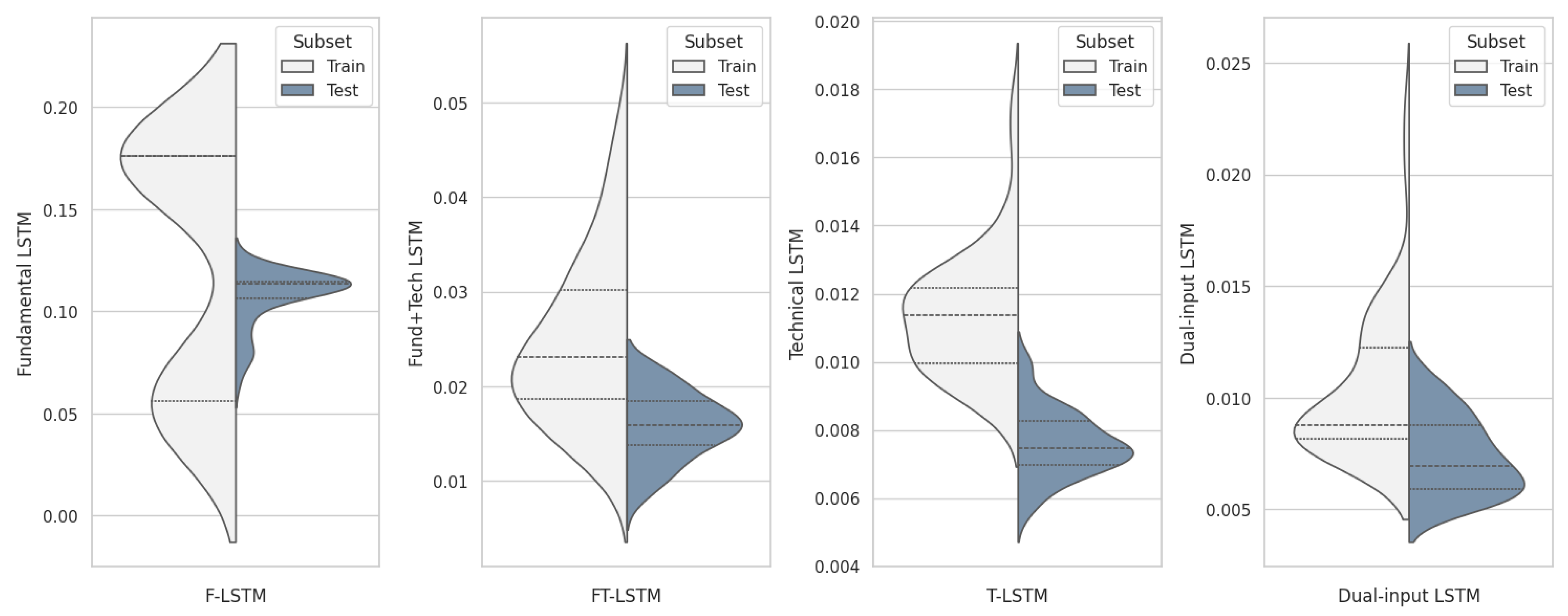
Figure 3 displays the
distribution on the training and test sets for the top 50 models in each group (those with the lowest test
). Quartiles are indicated by dashed lines: first (lower), second (inner), and third (upper). The plots confirm these findings. Considering the
y-axis scale, the models are ranked as follows:
To summarize, the F-LSTM model performs poorly in both trainability and prediction power, primarily due to the slower and less volatile nature of its predictors. This limited input hinders the model’s ability to capture dynamic market trends, making it unsuitable for reliable predictions. The FT-LSTM model performs somewhat better, yet it still lacks the foresight necessary for accurate forecasts, as combining fundamental and technical predictors has introduced complexity without fully capturing variability in the response variable. The mixed-input structure may have confused the model rather than enhance its predictive power.
The T-LSTM model ranks second overall in performance. Although it performs comparably to the dual-input model, its lack of crucial economic predictors limits its capacity to capture important variations in the response variable. In contrast, the dual-input model is superior in terms of trainability, prediction power, and computational efficiency. This model effectively integrates both fundamental and technical indicators, resulting in higher accuracy and robustness across both train and test sets. Consequently, the dual-input model is selected as the primary tool for generating three-day forecasts.
A traditional ARIMA-GARCH model [
52] was also employed for comparison, using the same 85–15% train–test split. The model development process proceeded as follows:
After differencing the training set by lag-1, the augmented Dickey–Fuller (ADF) test confirmed stationarity with a test statistic of −72.85 and a p-value of 0.000.
A grid search identified ARIMA as the optimal model based on AIC (−35,933.37), test RMSE (0.06678), and test MAE (0.05553), while ARIMA yielded the lowest BIC (−35,911.72).
Residual analysis on ARIMA confirmed mean-zero (Wilcoxon test p-value = 0.4984) and uncorrelated residuals (Ljung–Box test p-value for lags 1 to 12 all above 0.75) but identified non-normality (Jarque–Bera test p-value = 2.2 × ) and non-constant variance (Breusch–Pagan test p-value = 6.57 × ). The McLeod–Li test indicated volatility clustering, warranting a GARCH model to stabilize the variance.
The selected GARCH model improved residual diagnostics, with the Wilcoxon test indicating zero-mean (p-value = 0.5031), the Ljung–Box test indicating uncorrelated residuals (p-value for lags 1 to 12 all above 0.28), and the Breusch–Pagan test indicating constant variance (p-value = 0.205) but still failed normality tests. Thus, caution is advised when constructing normal-based confidence intervals.
The final ARIMA-GARCH
—
model demonstrated strong performance in training data with RMSE and MAE values of 0.0074 and 0.0055, respectively. However, on the test set, its RMSE and MAE of 0.0668 and 0.0555 showed limited generalizability, outperforming only the F-LSTM model and underscoring the superiority of the dual-input LSTM model. This model is formulated below while standard error of estimations is provided directly below the estimations.
where
represents the EUR/USD closing price at time
t,
denotes the differencing operation,
is the error at time
t,
signifies the variance of closing prices at time
t, and
represents white noise.
The GARCH component enhances the reliability of confidence intervals but does not contribute to trend estimation. Therefore, while useful for volatility assessment, the ARIMA-GARCH approach lacks the prediction power achieved by the dual-input model.
Additionally, using the same 85–15% train–test split and window size of 10, an SVM model [
23] was trained for comparison. Support vector machines (SVMs), as shallow networks with one or two hidden layers, often provide faster training than deep neural networks but may struggle with complex, noisy data, as is common in financial time-series.
The SVM model achieved training
of 0.05245 and
of 0.06711, with test
and
of 0.03265 and 0.04003, respectively. This performance ranks it better than the F-LSTM and FT-LSTM models but below the dual-input and T-LSTM models, indicating that SVMs, while efficient, may lack the adaptability required for complex financial prediction tasks (
Table 6). Default parameter settings included
,
,
, and an RBF kernel.
Using a ranked ANOVA Conover and Iman [
53], we computed the average rank (standard error) of
values for the top 50 runs of the LSTM models and a single run of the SVM model. The results are as follows: 67.9 (4.86) for dual-input LSTM, 85.2 (4.86) for technical LSTM, 213.7 (4.86) for Fund+Tech LSTM, 273.7 (30.82) for SVM, and 324.0 (4.86) for fundamental LSTM. Pairwise Tukey tests at the 5% family-wise significance level confirmed the model ranking as follows:
The consistent ranking across MAE and RMSE metrics in the training and test sets further emphasizes the robustness and superior predictive power of the dual-input LSTM model over both traditional and other machine learning models.
Forecasting Up to Three Days Ahead
As an additional layer of performance evaluation, 50 random points from the test dataset were selected. The top-performing models were then retrained for 200 epochs using 240 days of historical data and approximately two years of market activity, ending at the last observation before each selected test point. For these 50 forecasts, the and were calculated to be and , respectively. The of suggests that, on average, the model’s next-day predictions deviate from the actual values by just . These low and scores, obtained on randomly selected test samples, highlight the model’s robustness. Furthermore, the consistency with the original training results, where the dual-input model achieved both training and test MAE values below , reinforces the model’s ability to generalize effectively to unseen data.
Furthermore, to assess forecasting accuracy during the COVID-19 period, 50 random points between 2 March 2020 and 30 November 2021 were selected, and the same procedure was repeated using identical parameters. The RMSE and MAE of the next-day forecasts for these points were calculated to be and , respectively, further demonstrating the model’s stability and strong performance in forecasting under unprecedented market conditions.
The dual-input model, designed to incorporate both technical and fundamental indicators, was expected to perform well due to its ability to account for complex economic and market patterns. Retraining 240 days of recent data ensures that the model is exposed to recent market trends, which is essential for generating reliable short-term forecasts in a volatile market.
Figure 4 illustrates the next three-day forecasts generated as described in
Section 4.3. Using the best-developed model that achieved minimum
in the final training, the EUR/USD closing prices for 17–19 March 2025 were forecasted as
,
, and
. The high, low, and median prices in the boxplot were derived from the maximum, minimum, and median forecasts among the top-performing models that achieved
below
in the final training. At the time of these forecasts, the closing price on March 14 was 1.0879, while the actual closing prices for 17–19 March had not yet been released. The true values were later revealed to be 1.0921 (+0.39%), 1.0943 (+0.20%), and 1.0901 (−0.38%), respectively, indicating an upward trend followed by a downward dip. The forecasted values of 1.0873 (−0.06%), 1.0905 (+0.29%), and 1.0918 (+0.12%), respectively, predicted a slight initial decrease, followed by an upward trend that leveled off.
These results confirm the model’s forecasting performance, accurately capturing the overall trend direction and magnitude of changes with minimal deviation from the true values. The for these three forecasts is 0.0034, which aligns with the model’s prior performance assessments and further confirms its robustness.
This nuanced forecasting of both direction and fluctuation in EUR/USD pricing indicates the model’s effectiveness in capturing short-term market dynamics, making it a promising tool for practical trading or financial planning scenarios. Compared to simpler models, such as ARIMA-GARCH or single-input LSTM models, the dual-input model demonstrates superior accuracy, especially in capturing market turns over short forecasting horizons. This performance illustrates the advantage of integrating multiple indicator types in complex financial modeling, affirming the dual-input model’s utility in real-time financial forecasting and decision-making applications.
6. Discussion
A dual-input deep-learning LSTM model was developed to forecast the EUR/USD closing price using both fundamental and technical indicators. This model outperformed three alternatives: one with only fundamental indicators, one with only technical indicators, and one combining both but without the dual-input structure. The results confirm the effectiveness of combining these feature sets in a single input architecture for reliable forecasting.
Although the model was not trained for the binary classification problem of next-day price movement (Up/Down), it was evaluated for this task. After retraining the top-performing models on 240 days of prior data, the best model (, ) predicted the next-day price direction with 80% accuracy, correctly forecasting 40 out of 50 price movements. This suggests that the model can provide reliable directional predictions, though future work could improve this using a regression-classification framework.
Six technical indicators were selected from a broader set, including the commodity channel index (trend), awesome oscillator (momentum), and rate of change (momentum). Volume indicators were excluded due to a lack of reliable data. These technical indicators were chosen based on their relevance to market dynamics and model validation.
The fundamental indicators (federal funds effective rate, consumer price index, and gross domestic product for both the US and Europe) were selected for their correlation with inflation and long-term interest rates. Although they did not significantly improve performance, future work could explore including stock market metrics such as SP500 and DAX, which require separate forecasting. Using Shapley additive explanations (SHAP) statistics computed from the last 100 instances (default setting), we evaluated the contribution of each fundamental input feature to the output of the dual-input model. The results indicate that certain indicators, such as long-term interest rates and inflation in both Europe and the USA, consistently exert a stronger influence on the model’s forecasts compared to others, such as unemployment rates. These findings not only validate the economic relevance of the selected features but also highlight opportunities for potential model simplification and performance improvement.
While the dual-input model contains more parameters than the individual F-LSTM and T-LSTM baselines, it remains less complex than the FT-LSTM variant in terms of parameter count. The increase in training time compared to the FT-LSTM is, on average, less than three minutes, which is an acceptable trade-off between predictive performance and computational cost, especially considering the superior forecasting accuracy achieved by the dual-input architecture.
All fundamental indicators, except the European unemployment rate, showed significant (
correlations with EUR/USD closing prices. Multicollinearity affects time-series models, though not in the same way it impacts traditional regression models, such as multiple linear regression. This is because the primary objective of time-series models is not to interpret model parameters [
54] but rather to generate accurate forecasts. Moreover, LSTM and other deep learning models are nonlinear and can, in theory, learn to disregard redundant inputs. Unlike linear regression, these models do not rely on the assumption of independence between features.
With daily data, a window size of 10 captures approximately two weeks of market activity, which is generally regarded as a medium-range interval. Although we experimented with various window sizes during the validation phase, a more comprehensive investigation could help identify the optimal window size for next-day price forecasting. While the model can predict up to nine days ahead with a window size of 10, forecasts become less reliable over longer periods. A more robust approach would involve daily retraining to incorporate new information.
The observed decline in prediction accuracy over extended time horizons highlights a key challenge in time-series forecasting. This issue may stem from the model’s inability to adapt to evolving market dynamics and the accumulation of prediction errors over time.
Training multiple models on different time scales, such as daily, weekly, or even monthly, can help the system better capture trends across various temporal horizons. By incorporating longer-term patterns, the model gains a broader contextual understanding of market behavior, which in turn helps smooth out sudden shifts or anomalies that may appear on shorter time scales. For example, a daily model might overreact to short-lived volatility or noise, whereas a weekly or monthly model can provide a more stable reference, acting as an anchor for trend direction. This multi-scale approach not only enhances robustness but also improves the model’s ability to generalize and adapt to different market conditions.
Furthermore, exploring hybrid modeling approaches that combine statistical time-series models (e.g., ARIMA) with deep learning architectures could also be beneficial. Statistical models are adept at capturing long-term trends, while deep learning excels at modeling complex, non-linear relationships. A hybrid approach could leverage the strengths of both methodologies, leading to more robust and accurate long-term predictions.
7. Future Work
While LSTM models have demonstrated effectiveness in capturing temporal dependencies, emerging architectures such as transformers, leveraging self-attention mechanisms [
55], present an intriguing avenue for future research.
Transformers excel at modeling long-range dependencies by directly attending to all positions in the input sequence, overcoming the inherent limitations of LSTMs in handling very long sequences where information decay can occur. The self-attention mechanism allows the model to dynamically weigh the importance of different parts of the input, potentially capturing subtle but crucial relationships that LSTMs might miss. Furthermore, the parallelizable nature of transformers could lead to significant computational efficiency gains, particularly for large datasets.
Future work could explore integrating Transformer layers with LSTMs to create hybrid architectures. For instance, a transformer could preprocess the input sequence to extract global contextual features, which are then fed into an LSTM for finer-grained temporal modeling. This hybrid approach could combine the strengths of both architectures: the long-range dependency modeling of transformers and the sequential processing capabilities of LSTMs, potentially leading to substantial enhancements in predictive accuracy. Additionally, investigating the application of sparse attention mechanisms within transformers could further improve efficiency and robustness, especially when dealing with high-dimensional time-series data or sequences with varying lengths.


