1. Introduction
The radial bases function (RBF) network is an important network architecture, introduced in 1988 [
1]. In RBF neuron forward processing [
2], the positions of the objects are based on the distances from the given centroids. The neurons correspond to spherical areas in the object space, and the associated activation value depends on the distance to the centroid of the radial neurons.
According to the analysis performed in [
3,
4,
5], the main benefits of the RBF network can be summarized as follows:
relatively simple architecture,
low parameter complexity,
fast learning process,
strong tolerance to input noise,
good generalization ability.
The conclusion of the comparison of the RBF network and traditional MLP networks ([
4]) shows that:
RBF networks are especially recommended for surface with regular peaks and valleys;
For classification problems, traditional neural networks can usually provide better classification results;
RBF networks perform more robustly and tolerantly than traditional neural networks when dealing with noisy input data.
In traditional RBF networks, the activation at node
i is calculated with a Gaussian function:
where
denotes the centroid of the neuron. The parameter
corresponds to an inverse radius value that determines the slope of the activation curve.
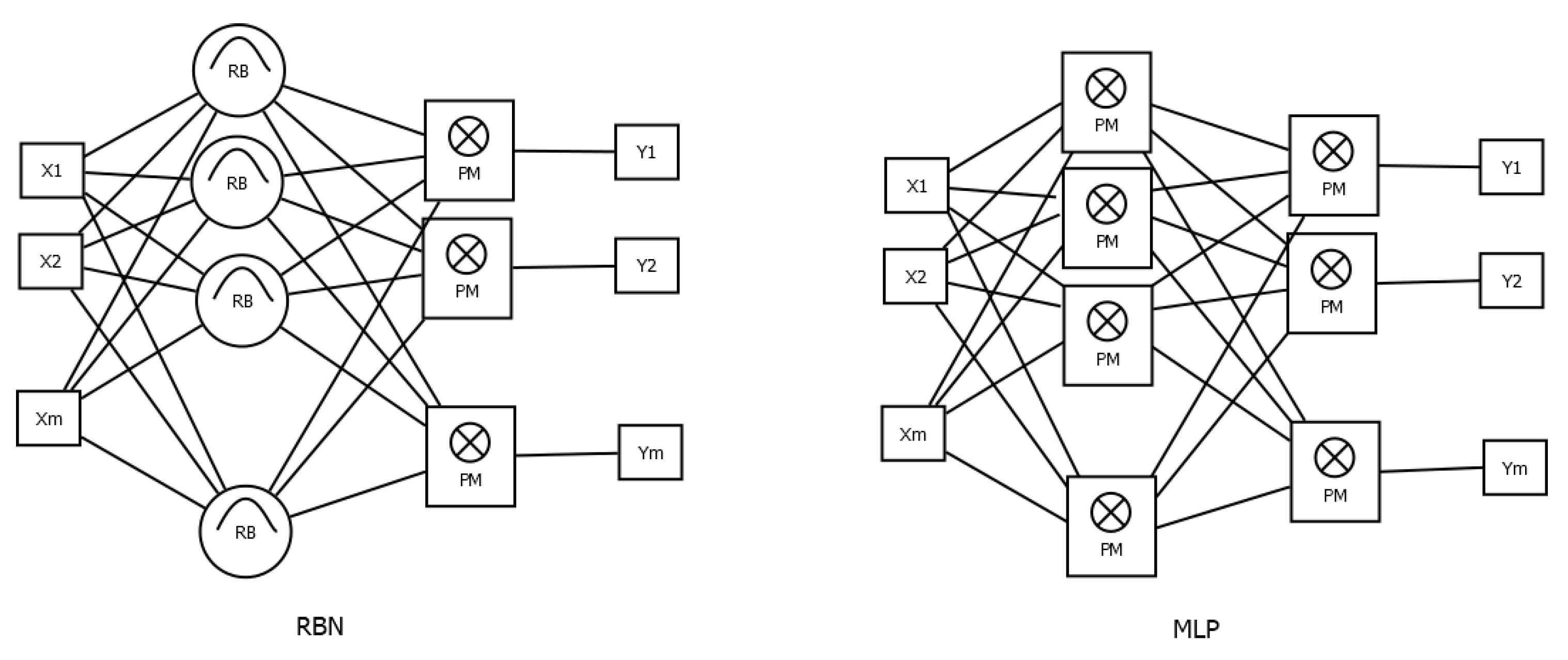
The RBF network has a three-layered architecture, including:
an input layer, which represents the feature vector of the input items;
a middle layer of radial neurons;
an output layer, where each neuron corresponds to an output category.
The layers in the network are fully connected. The baseline forward process is performed in two phases. First, the feature vector of the objects is transformed into a vector of activation values of the radial neurons, then this vector is sent to a standard perceptron layer. The output signal in the output layer is computed based on a linear weighted sum of the outputs of the radial neurons. An architecture comparison of the RBF network and the baseline MLP network is presented in
Figure 1.
Due to the benefits of RBF networks, we can find many publications in the literature on the practical application of RBF networks. In [
5], the network is applied for dynamic system design, where the authors presented novel learning methods using error correction with the second-order gradient approach. The robust decision surfaces and the ability to estimate the distance a test case is from the original training data were the main reasons to apply RBF for fault diagnosis (see [
6]). In [
7], a rain prediction framework was developed via integration of evolutionary optimization methods with RBF backpropagation methods. Another special application field is presented in [
8], where a novel RBF-based neural network method was applied to solve elliptic boundary value problems. There are many other application areas in the literature, such as time series prediction [
9], earth science [
10], human–computer interfaces [
11], or engineering [
12].
In the literature, the efficient construction of the RBF neural network architecture is an actively investigated research domain. Considering the key research projects on RBF, we can identify the following key research directions:
form of the kernel function,
initial positions of the centroids,
learning algorithm.
One of the recent key results [
13] shows that large RBF networks with suitable optimizers, regularization techniques, can achieve predictive performance comparable to gradient-boosted decision trees.
Although in current research activities on neural network technology, the MLP and convolutional neural models are the dominating methods, the number of research works on RBF network models has still been increasing in recent years [
14]. This fact shows that, thanks to the recognized benefits, the RBF model plays a stable and important role in the family of neural network models. The current RBF applications are based on the overriding principles of k-means variant clustering and two-phase parameter optimization. Another interesting fact, that there is a large separation between the RBF and other traditional neural network models, is that the RBF is considered as a model with a fixed, relatively rigid architecture. It is widely assumed that the RBF has a weaker classification accuracy but better stability.
Considering the initial positions of the centroids, there are the following main initialization approaches [
15] in the literature:
uniform or random distribution,
unsupervised clustering methods,
supervised clustering (usually the decision tree method),
evolutionary optimization algorithms (here, the GA is the dominating approach).
Regarding the radius parameter of the radial neurons, the usual solution is to use a single value for all neurons. In the more sophisticated variants, the following solutions are used:
Hyper-basis functions are defined with the following formula [
16]:
where
is a positive definite matrix that determines the contour of the related border hyper-ellipsoid.
Considering the initialization of the
value, the most general solution is to set the value to the mean of distances to the nearest centroid [
15].
Regarding the weight parameters of the links that connect the radial and output layers, the dominant solution is the application of the standard backpropagation training algorithm [
17]. A more special algorithm was presented in [
15], where the calculation of the weights between the middle and output layers was performed with a least mean square error procedure using Bayesian decision optimization, which assumes that the output of the middle layer forms a normal distribution. Another interesting approach is presented in [
3], and a new kernel function is proposed, which is a composite of a set of sigmoidal functions that aims at approximating a given function with nearly constant values.
The primary motivation of our research was to analyze the integration of RBF and MLP neural network models, with the aim of developing an efficient hybrid model that takes advantage of the strengths of both approaches. The main contributions of this work are:
The introduction of a new measure for the evaluation of centroid positions. The measure value is based on the homogeneity and density of the neighborhood region.
The development of a novel initialization method for RBF networks.
The development of a novel network architecture combining RBF and MLP modules.
The implementation and presentation of test cases that show the superiority of the proposed architecture.
2. Rbf Centroid Initialization Based on Distance-Weighted Homogeneity
2.1. RBF Centroid Initialization Methods
The simplest approach is the random initialization approach, usually using a uniform distribution. The main drawback of this approach is that the real category distribution in the object space is not uniform. According to the test results in [
18], random initialization of the centers could lead to misclassification and biased approximation, providing weaker precision than the other approaches.
In the case of unsupervised clustering, the k-means method is the dominant variant [
19]. Although random positions are generated in the first phase, in later steps, the positions are improved by the optimization algorithm to minimize the intra-cluster distances:
where
is an object vector in the feature space and
is the centroid to which
belongs. The symbol
denotes the Euclidean distance. In the baseline versions, the k-means clustering focuses on finding dense areas in the feature space where the category assignments of the objects have no role in the positioning of the centroids. In this sense, clustering is an unsupervised optimization approach. In the literature, we can later find approaches in which the clustering is performed in separate steps for each category [
15]. This means that centroids represent homogeneous clusters in the object space. Another extension is to apply some other heuristics in the clustering process, such as the immunity-based approach (immunological center selection, [
18]). This method uses an affinity measure that is inversely proportional to the distance and generates centers with high affinity values using center cloning and pruning operations.
The execution complexity of the k-means clustering method can be approximated as follows:
where
N is the number of objects;
D is the dimensionality of the object space;
K is the number of clusters; and
I is the iteration count [
20]. The value of
I is hard to predict, as it is significantly dependent on the distribution of the data and the initial position of the centroids. One of the key novelties of the k-means++ method is that it applies an optimized centroid initialization method. Although k-means clustering is a widely accepted method, there are some shortcomings that can degrade its performance. One issue is that it is suitable only for clusters with homogeneous density values; its assumption of spherical and equally sized clusters results in insensitivity to the category distribution of the objects.
In the case of the k-means method, the objects are assigned to the nearest centroid, independently of the distances to the other centroids. If the difference between the shortest distance and the second-shortest distance is small, this crisp decision will eliminate significant information. In the proposed fuzzy version of the k-means, the c-means method, the nodes belong to more different clusters at the same time. As the management of these relationships requires more calculations, the complexity of c-means is higher than the complexity of the k-means method:
In general, the c-means method has similar problems as the k-means and it is also sensitive to local optimums.
Tree structures can also be used for clustering. The R-tree is one of the most widely used methods for this task. It constructs nested rectangle areas as clusters. The main cost factor in building the R-tree [
21] is the splitting of a cluster into two sub-clusters. The cost complexity can be approximated as follows:
In some versions of tree structures, category homogeneity is also involved in the node split operation. Tree construction is a relatively fast method, but the generated partitioning is of lower quality.
In the family of decision trees, the most popular choice is the application of the C4.5 method [
22]. In the tree, every leaf node is associated with a rectangle area whose center is selected as the centroid. In the case of optimal decision trees, the set of objects assigned to the nodes has optimum homogeneity. The homogeneity is usually measured with some variants of entropy on the category labels. Thus, the decision tree approach strives to position the centroids in homogeneous clusters.
In some versions of the tree structures, the category homogeneity is also involved in the node split operation. Tree construction is a relatively fast method, but the generated partitioning is of lower quality.
In [
23], the optimal positions of the centroids are calculated with a clustering algorithm, APC-III. This method is a variant of quality threshold clustering, as it assigns the items to the nearest cluster if the distance is below a threshold; otherwise, the item will be considered as center of a new cluster. In order to avoid heterogeneous clusters, the clustering is performed separately for each category.
As shown in the analyses performed [
24], supervised clustering provides many advantages over standard unsupervised methods. One simple approach to consider the category is to extend the object feature vectors with a new dimension describing the category label [
25]. One disadvantage of this method is the difficulty in normalizing the values of two vector sections. Another method is the application of output context clustering [
26]. The algorithm first defines the output contexts and then clusters the inputs with their respective output contexts. This method guarantees that all elements of a given cluster belong to the same category.
This method was extended by [
24], where a module was introduced to determine the optimal number of clusters for a regression problem. The goal of the extension is to separate similar input objects belonging to the same category from the rest of the dataset. The method first generates disjoint intervals of the value set. The objects are then assigned to the corresponding value interval. The sets obtained are homogeneous in terms of output value (category). For each category object set, fuzzy c-means clustering is invoked to find the optimal initial positions of the related centroids. As objects of the same category are usually distributed in many local clusters, the main task of the proposed module is to find an appropriate set of sub-clusters for every category. The optimization module applies a novel separability factor to find the appropriate subcluster number.
Regarding evolutionary methods, we can see a wide variety of heuristic methods, such as the genetic algorithm [
27] or swarm optimization methods [
28]. Some of the main drawbacks of this approach are the following:
high execution cost,
low stability.
The analyses performed found in the literature show that the appropriate initial location of the centroids is a key factor in the efficiency of the redial basis neurons. A important step in the development of an efficient RBF unit is to find an optimal position in the object space.
The main problem of all traditional initialization methods is that they are insensitive to the category distribution. Considering, for example, a uniform or a baseline k-means initialization, the methods do not take into account the category labels. If the centroid is located in an inhomogeneous zone, the generated activation signal has a low category separation power, and it cannot significantly improve the classification accuracy of the neural network. On the other hand, if the spherical area of the redial function neuron includes a homogeneous zone, the unit has high activation signal output only for the related single category; thus, this unit has a high separation power.
As existing methods lack the ability to locate the optimum position for a wide range of problem domains in an efficient way, the present work focuses on the presentation of a novel approach for centroid initialization to find homogeneous dense zones in the object space.
2.2. Initialization of the Centroids with the DH Measure
In our investigation, we focus only on the classification problem, where objects are assigned to discrete categories. First, we introduce a homogeneity measure to evaluate the different positions in the feature space. The proposed d-entropy (or density-based entropy) is used to measure the homogeneity related to a given position in the feature space T.
D_entropy. Having a set of labeled objects
, where
is the position (feature vector) of the object and
is a category label, the d_entropy at position
is calculated as follows:
where
i denotes a category index and
. The value of
is given as follows:
denotes the objects belonging to category
c, and
is the selected distance (usually Euclidean distance) function in the feature space.
For the demonstration of the density entropy, let us take a one-dimensional object space with the following data distribution:
category A: [0.1, 0.15, 0.18, 0.20, 0.35, 0.43]
category B: [0.3, 0.4, 0.5, 0.6, 0.65, 0.8]
The proposed measure D_entropy(x) shows the homogeneity of the category in the neighborhood of
x. The shape of the calculated homogeneity measure for various gamma values is illustrated in the following figures (
Figure 2 and
Figure 3). In the figures, the two bottom lines of the circles show the positions of the data items. As we can see, the homogeneity value is significantly dependent on the gamma factor. If gamma is near zero, the neighborhood is very large, and each position has the same homogeneity value. The higher the gamma value, the smaller the neighborhood area. The proposed RBF initialization method will focus on locating homogeneous areas, where the (low D_entropy) measure is minimal, to position the RBF centers. The main idea behind this step is that the accuracy of the RPB prediction is better in homogeneous areas than in inhomogeneous areas.
The introduced D_entropy measure has a low value if the neighborhood of the argument position is homogeneous regarding the category labels. The base features of the D_entropy measure can be summarized on the basis of the following properties.
Proposition 1. If the object set is homogeneous, only one category is present, and the value of D_entropy is equal to zero for every position .
This property is based on the fact that and = 1.0.
Proposition 2. For every object space and position: This statement follows directly from the definition.
Proposition 3. In a finite bounded object space, ifthen the D_entropy approaches the Shannon entropy of the object set. In this case, we obtain
and thus
and
Using the limit value of
, we obtain the Shannon entropy value.
Proposition 4. If for every object in the object setthen the D_entropy(x) value is equal to the Shannon entropy of the object set. Similarly to the previous proposition, we obtain
and
Thus, we obtain the Shannon entropy as the result.
As we can see, the proposed measure has some formal similarity with the Shannon entropy concept, as
both have similar formulas,
the distribution of is similar to the probability distributions,
both can be used to find homogeneous sets.
The factor determines the radius of the sphere of the effective zones. If is too small, there is a large effective zone and all positions in the space tend to be of similar importance. The other extreme is when is too large; in this case, the effective zone is restricted to a single point.
The D_entropy measure can be used to show the homogeneity level of the different locations in the object space, but this measure alone is not powerful enough to reach the main goal, namely to locate dense and homogeneous areas. Thus, in the next step, we add a density component to the measure to improve efficiency.
DH-measure: For a set of labeled objects
, where
, the DH measure at position
, (
) is defined as
where
and
is a weighting factor.
The expression can be considered as a measure of density homogeneity in the feature space. In the optimal position, the value is at minimum, i.e., the density measure is high and the D_entropy part is low.
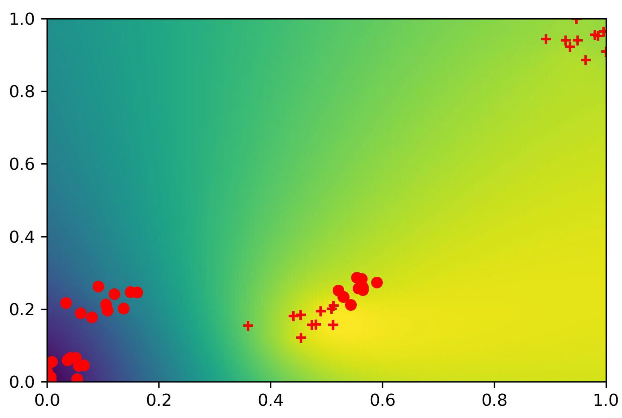
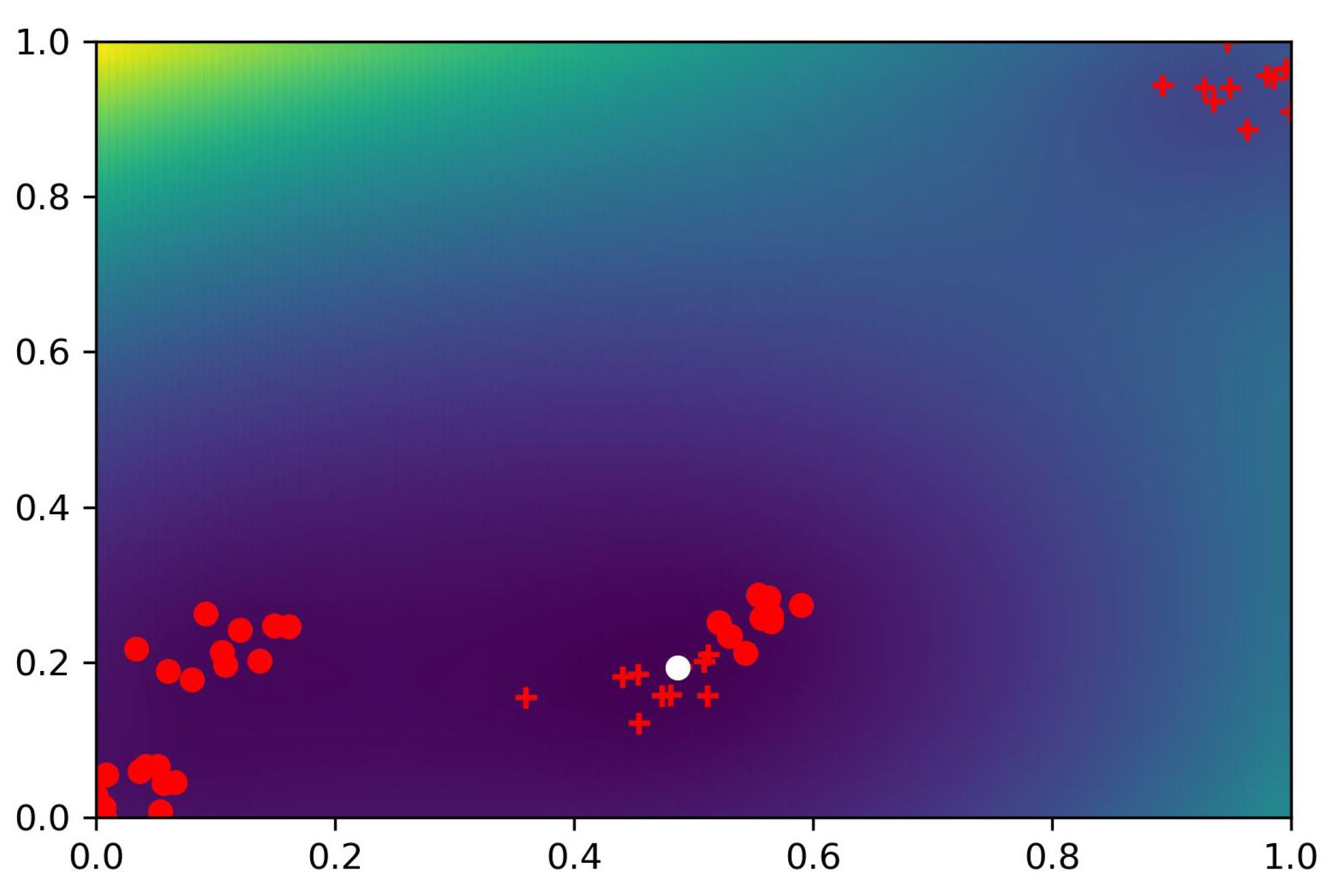
Example 1. In the next figures (Figure 4 and Figure 5), a simple two-dimensional feature space is tested to illustrate the shape of the D_entropy measure for different γ factors. The objects in the dataset are organized into blobs. There are only two categories; the related objects are denoted by + or o markers. The figures show the related heat maps for different γ values. We can observe that the larger γ values represent steeper slopes for the D_entropy function. In the figures, the light colors show high density values, while dark colors denote small density areas. Example 2. In the next examples (Figure 6 and Figure 7), the heat map of the D_entropy measure is illustrated for the same object space. We can also observe here the effect of the γ value on the shape of the heat map. Example 3. In the third example (Figure 8 and Figure 9), the heat map of the DH measure is illustrated for the same object space. In the figures, the white circle shows the position of the optimum value. The measures introduced will be used to find the optimal initial centroid positions of the neurons of the radial basis function. As full scanning of the whole object space is usually impractical, we present an approximation method in the next section.
2.3. Initialization of the Radial Function Neurons
In order to avoid the full scan of the entire object space, the proposed method applies a widely used simplification approach, namely, the search is not performed on the whole universe
, only
, the set of object positions tested. We assume that the number of centroids required is fixed and is denoted by
K. If we were to take the first
K objects having the best DH-measure values, we would usually obtain positions near each other, which would degrade the efficiency of the RBF layer. In order to avoid this risk, an additional parameter
is introduced which corresponds to a threshold value: the distance between two centroids must be greater than
. The selection of the centroid objects is carried out using the following algorithm (
Figure 10).
Calculate the DH measurements for all elements of the set of objects and introduce O as the set of candidate objects. Initially, O is equal to the set of objects in T.
Select the object with the minimal DH-measure value as the first centroid.
If the number of centroids in S is equal to K or o is empty, then the algorithm terminates.
Remove the
-neighborhood of the centroid recently selected from
O (
).
Select the object with the minimal DH-measure value as the next centroid.
Go to Step 3
Based on the literature, the standard step after initialization of the centroid positions is the application of the iterative (usually back-propagation) algorithm to optimize the weight values between the RBF layer and the output layer. As the process starts with a random weight distribution in the perceptron layer, this process takes more time to find the appropriate weight setting.
2.4. Weight Initialization of the Perceptron Layer
In our opinion, the process of weight learning can be sped up with a method based on the following considerations. If we find the optimal centroid position, then its neighborhood will contain homogeneous objects that belong dominantly to a given category c. Thus, for every centroid, we can determine a dominating category, or more precisely, we can calculate a weight value for all categories based on the values used in the calculation of the D_entropy measure. In the proposed method, we use these values as initial weight values for the edges between the RBF and the output layer. With this kind of initial setting, the RBF neuron will send a strong signal to the category neurons that dominate its neighborhood. Thus, in other words, if the test position x is in the neighborhood of the centroid s and the relative frequency values of the categories are equal to , then the importance of the centroid output in the different output neurons is proportional to ; thus, the dominant categories in the RBF centroid will obtain the highest input signal.
The initialization of the edge weights is performed in the following steps.
In the proposed novel two-phase initialization model, the first phase is to find the optimal centroid positions using the HD-measure as the objective function. In the second phase, the weights of the outgoing edges are set equal to the relative frequency vector values calculated in the first phase optimization process. The main promise of this method is that it can ensure better initial accuracy of RBF network classification.
Proposition 5. The probability of correct prediction is higher for the proposed bounded two-phase initialization method than in the case of random weight initialization.
To show the correctness of this proposition, let us take an RBF layer with centroids . The input target object is denoted by x, and we assume that x belongs to the neighborhood of . The set of categories is given by . We assume that the probability order at z is . The activation signal of neuron is denoted by , . The related relative frequencies at centroid are . The weights for the outgoing edges are denoted by . If the values are generated uniformly randomly, the , ,…, vectors are independent and belong to the same value domain, having the same value distribution.
The output of the category
j in the output layer is calculated with:
This means that the expected value of the output values
for the different categories has the same value. This means that each category has the same chance to be the winner at the output layer. In this case, each category has the same
probability of being the prediction value.
In the case of the DH-measure approach, the weights are equal to the density factors:
Taking into account the output values, we can use the following formula:
As the
vectors are independent and correspond to the same value distribution, the average value for
is the same for each category. On the other hand, as
and
we have
This means that for an average case, the prediction for x is the category . As this category has the highest chance in the region of , the expected accuracy value is higher than for the random case, where each category has the same probability of being selected as the winner.
2.5. Parameter Optimization
The efficiency of the position initialization process and the classification prediction significantly depends on the two key parameters of the proposed algorithm, namely the gamma factor () and the cluster count (K). In order to provide an optimal parameter value selection, we performed a combined hill climbing optimization process. In the first step, we determine the reasonable value range using the following heuristic considerations:
If gamma is too small, near 0, all positions have very similar fitness values.
If gamma is too large, the neighborhood is restricted to only a few other points.
If K is too small, we obtain a weak approximation.
if K is too large, the execution cost and overfitting increases.
According to our experience, the optimal parameter values depend on the data distribution; thus, we involved different data distributions in the optimization tests. For the gamma parameter, we selected two starting points in the optimization process: . In both cases, we obtained nearly the same results with . We can remark that this gamma value also provided the fastest convergence in the training process of the constructed neural network. Regarding the K parameter, the minimal value was 10, and the largest value was 100. Here, as expected, the setting provided the best convergence in the training phase, but considering the overall cost values, we found that K = 50 was the optimal cluster count for the investigated datasets.
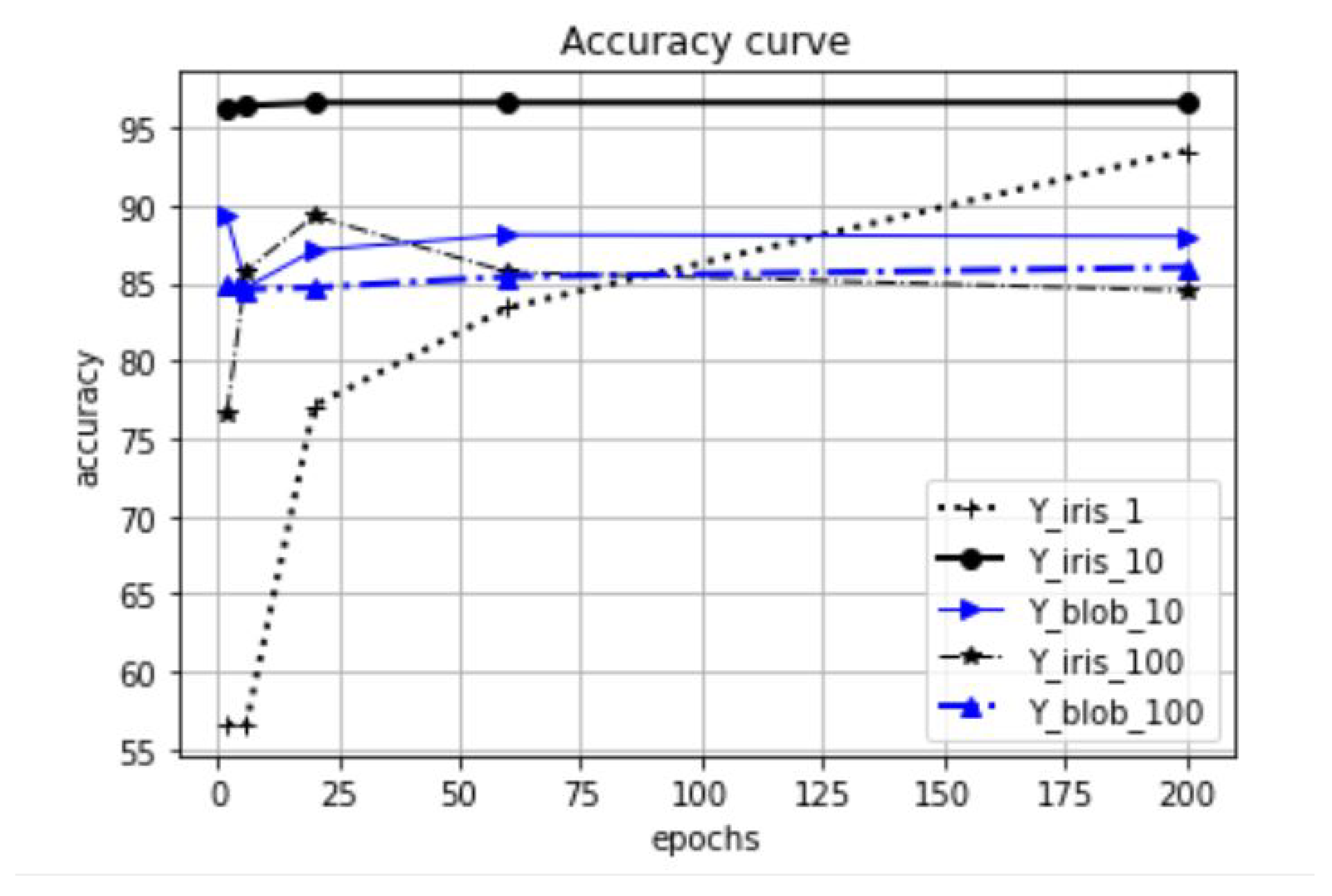
2.6. Test Results
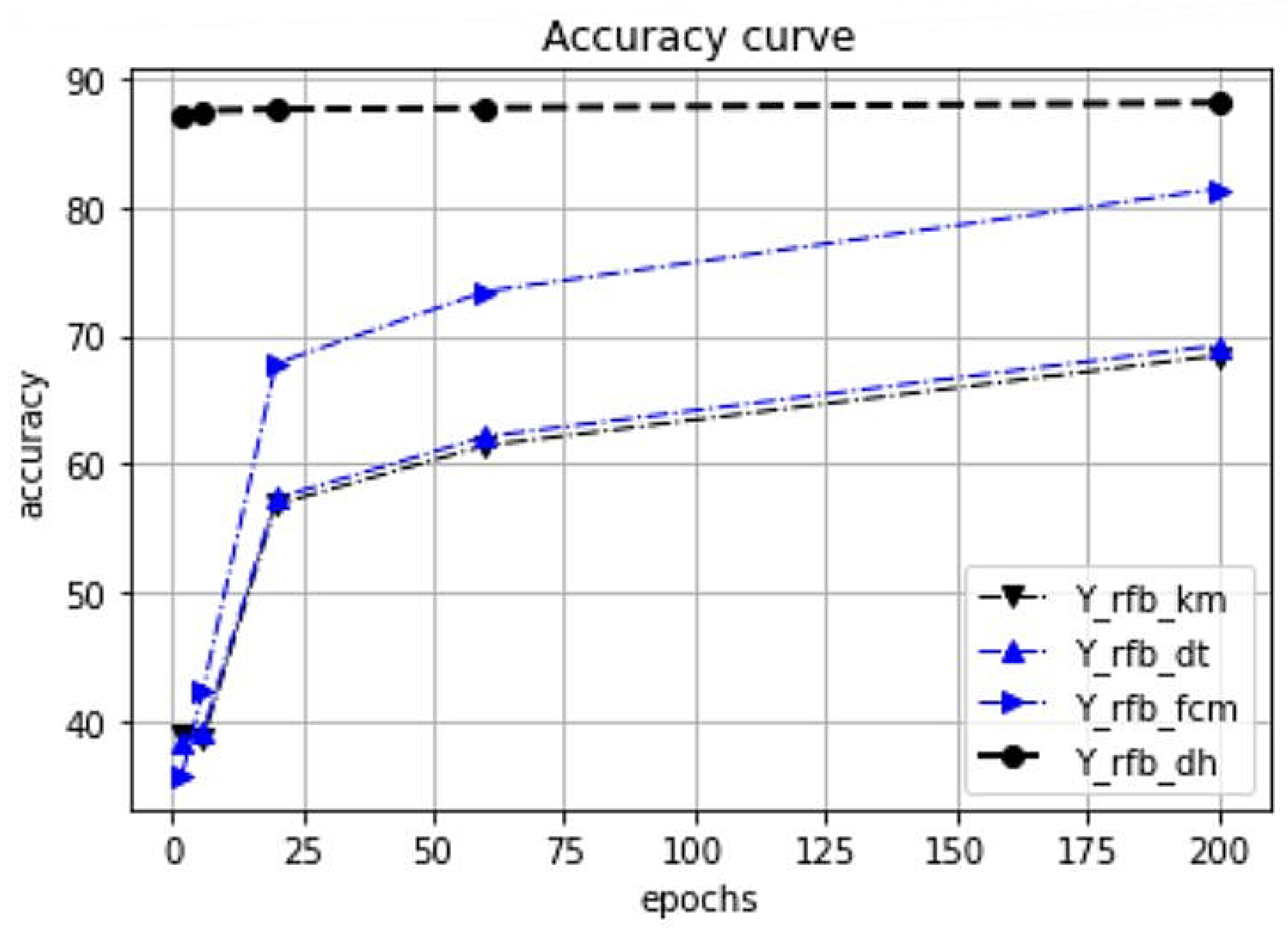
The main goal of the next experiments was to compare the classification accuracy of the proposed DH-based RBF models with the standard RBF initialization variants. In the tests, the following RBD variants were involved:
RBF-KM: baseline RBF structure with k-means initialization,
RBF-DT: RBF structure with decision tree initialization,
RBF-FCM: RBF structure with fuzzy c-means initialization,
RBF-DH: the proposed RBF model.
Regarding the test datasets, the following benchmark databases were involved in the experimental tests:
In the list, the symbol M denotes the number of attributes, C denotes the number of categories, and N shows the number of records in the dataset. In the case of the Uniform dataset, a uniform random distribution in a hypercube was used to generate the objects. The objects in the Blobs dataset are distributed in clusters using the make_blobs routine in the sklearn Python package.
The test framework was implemented in the Python infrastructure. The main goal of the performed tests was to compare the accuracy level of the existing and novel approaches on some widely used benchmark datasets.
The test results are summarized in
Figure 11,
Figure 12,
Figure 13 and
Figure 14. As we can see from the result data, the proposed initialization method provides a fast learning rate even after the first few epochs. For datasets with a clear cluster structure, the proposed method provides faster and more efficient learning. The benefits of this approach are very significant, especially for well-clustered object distributions such as the case for the Blob dataset.
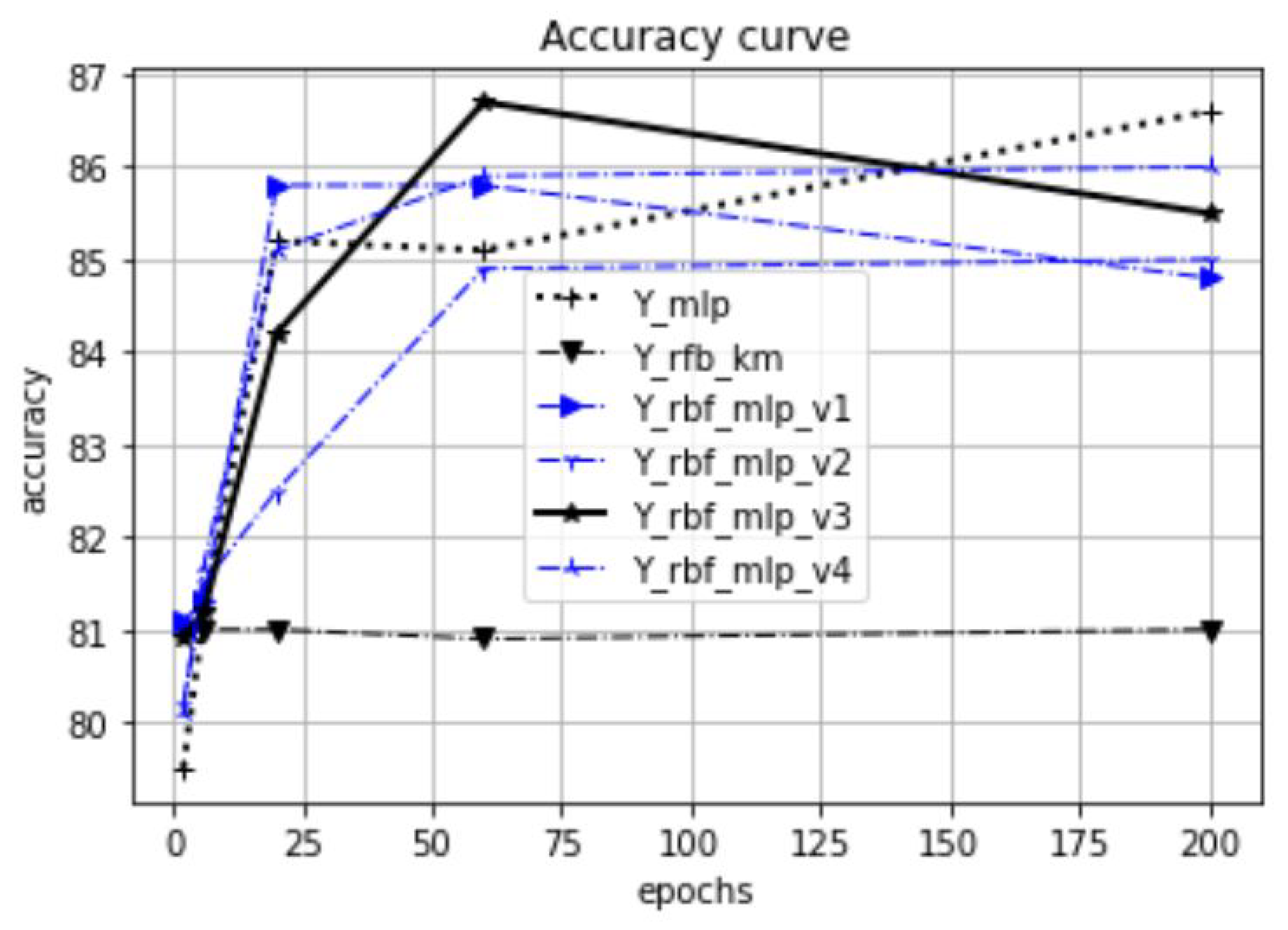
4. Test Experiments on the Integrated Architecture
The main goal of the experimental tests is to compare the classification accuracy of the proposed integrated models with the standard variants, RBF and MLP. In this section, we use the following abbreviations to denote the different network architectures.
Existing architectures:
MLP: baseline MLP structure with a single hidden layer,
RBF-KM: baseline RBF structure with k-means initialization.
Investigated novel architectures:
RBF-DH: the proposed RPF model;
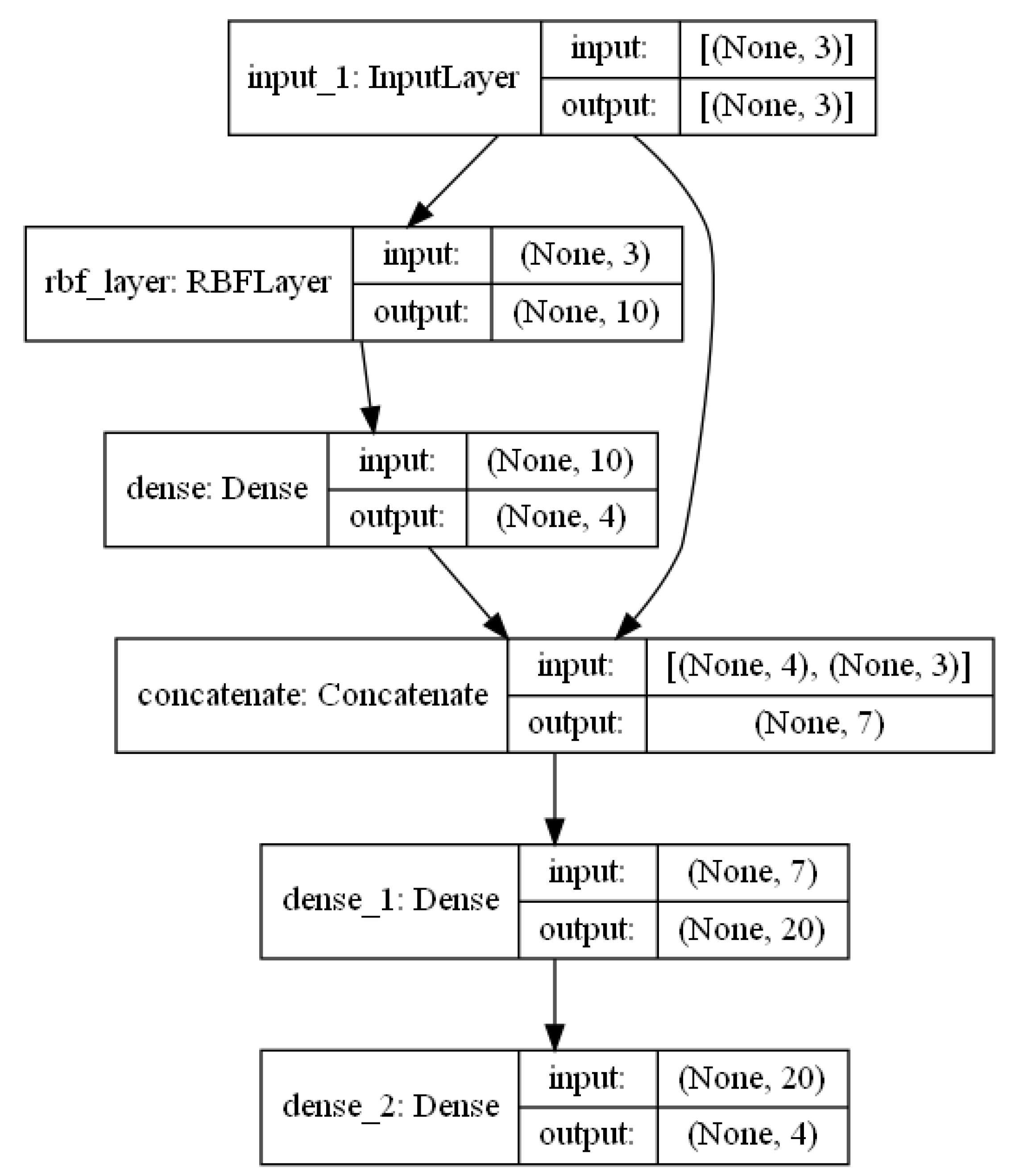
RBF-MLP-V1: integration of proposed RBF with MLP version 1;
RBF-MLP-V2: integration of proposed RBF with MLP version 2;
RBF-MLP-V3: integration of proposed RBF with MLP version 3;
RBF-MLP-V4: integration of proposed RBF with MLP version 4.
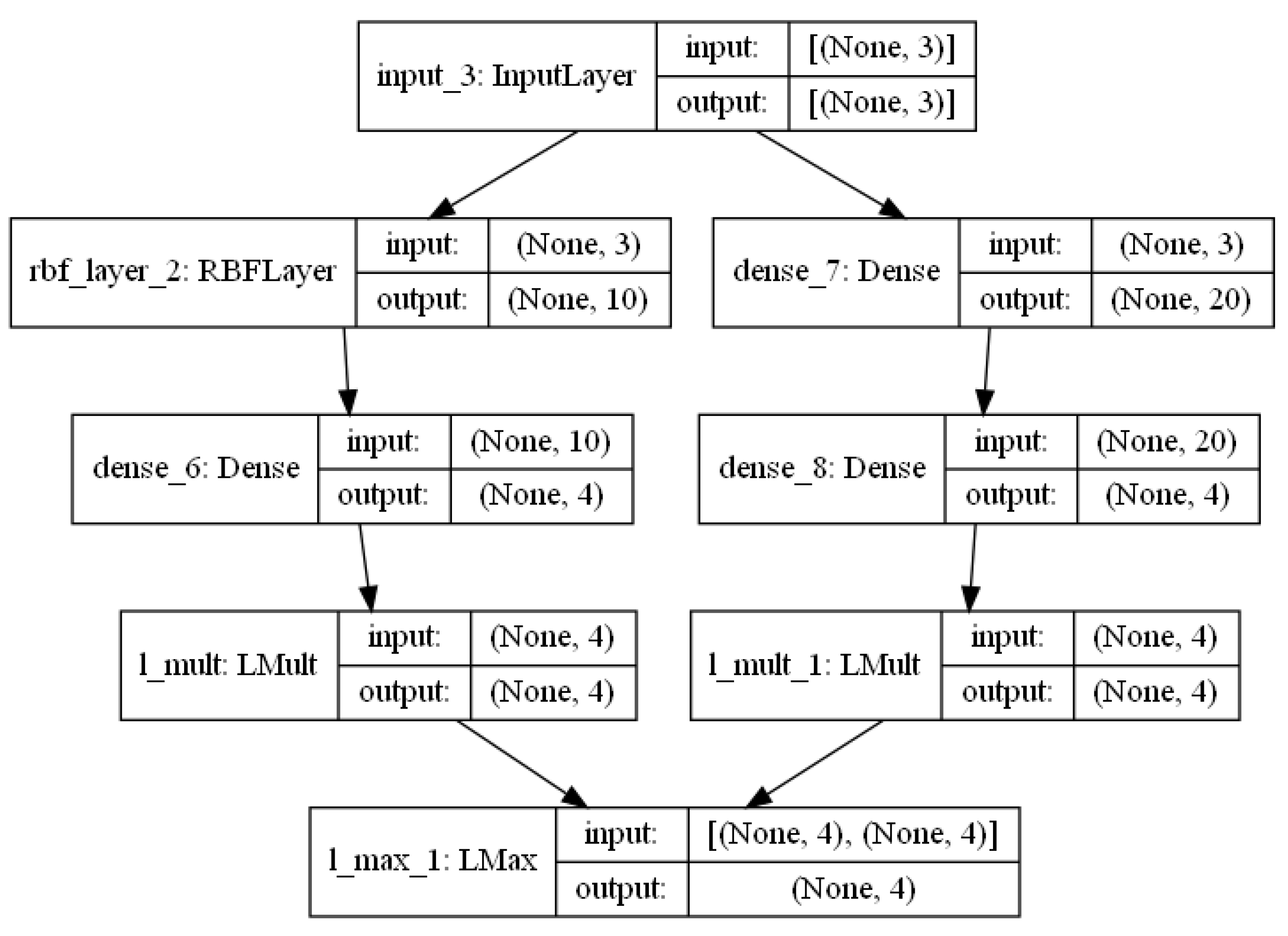
The RBF-MLP-V4 version contains two separate networks, an RBF and a MLP module. For a given object
x, the engine calls the RBF neural network if the object
x is near a centroid (
—distance threshold); otherwise, the MLP unit is used for prediction. The measured values are presented in
Figure 18,
Figure 19,
Figure 20,
Figure 21,
Figure 22,
Figure 23,
Figure 24,
Figure 25 and
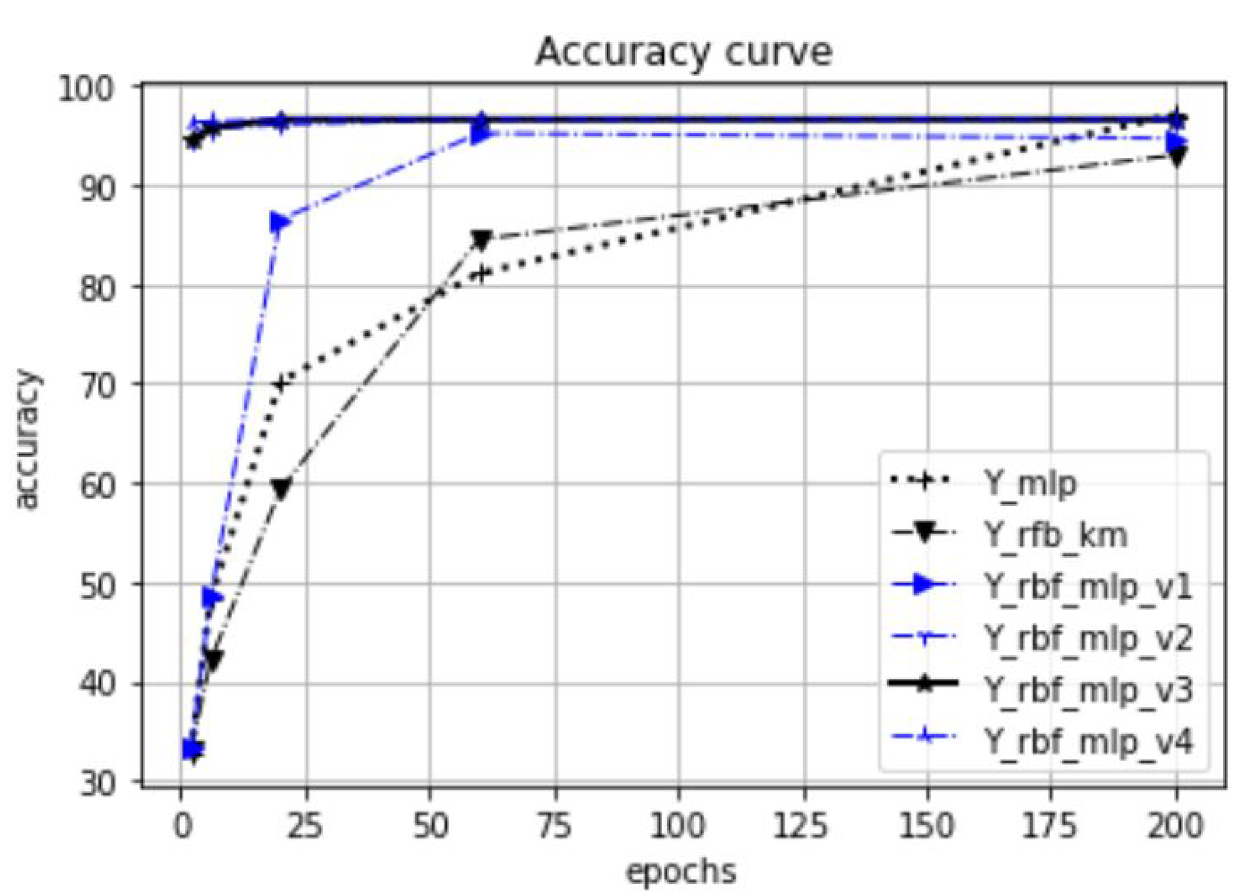
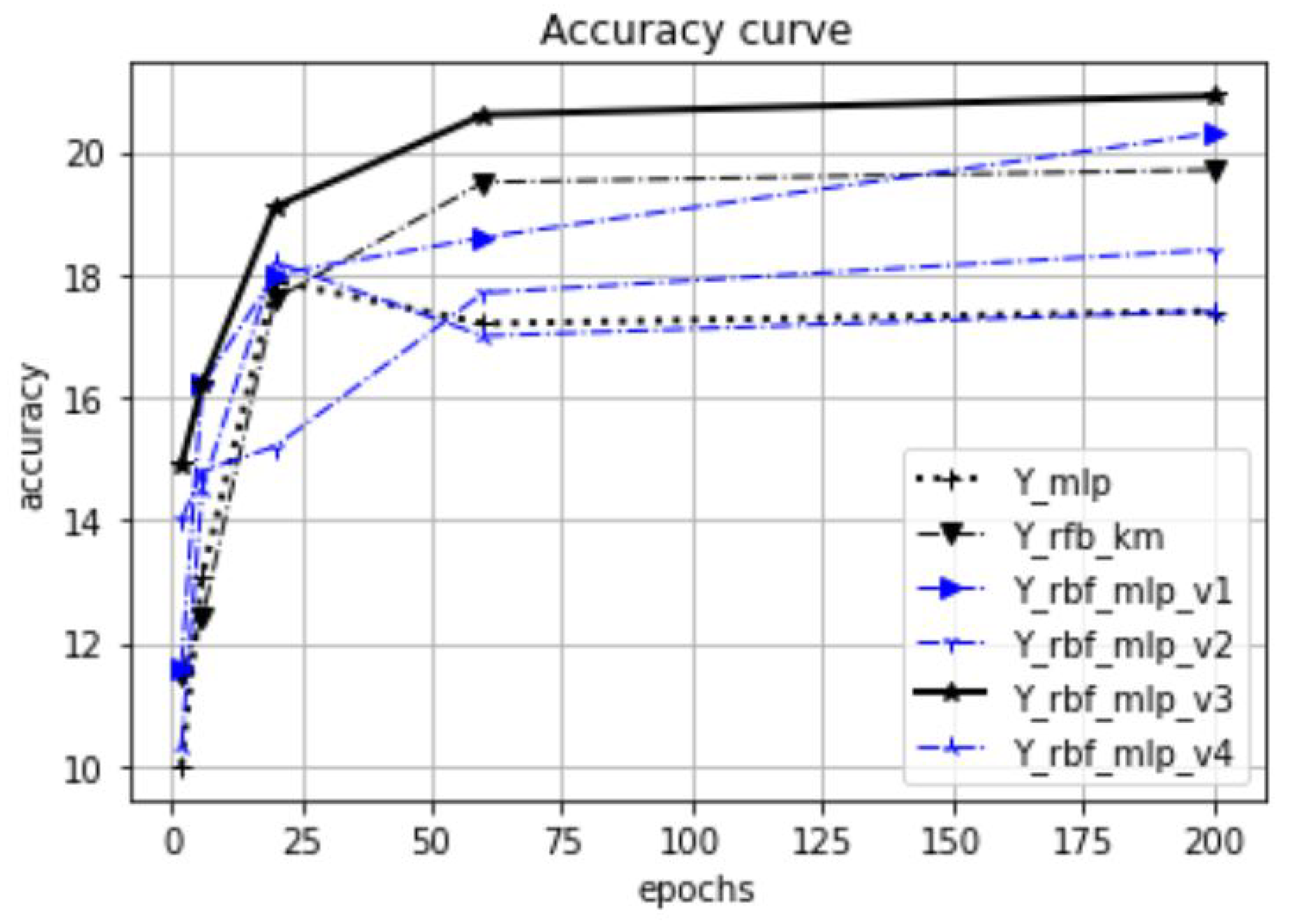
Figure 26. The accuracy values presented in the results are the calculated average values based on 20 measurements. Our focus is on investigating the effect of the proposed initialization method, especially at the beginning of the training process. Therefore, in our experiments, the test accuracy was measured as a function of the preceding epoch steps. Thus, we selected five epoch lengths (2, 6, 20, 60, 200), performed training with these epoch settings, and called a test evaluation after the training phases. For the tests, we used 20% of the available datasets, and 80% was used for training and validation.
In
Figure 18, the dataset is the synthetic Blob object set in 10-dimensional space. The test was executed with
. Each dataset is represented with one figure related to the common epoch range. The title of the figures shows the dataset name, the number of dimensions, and the
values. These figures relate only to a part of the performed tests; the total number of perfomed tests was 122. In these tests, we analyzed, in addition to the epoch dependency, among others, the
-dependency and the
K-dependency. The full list of the test results can be found in URL_meresek.
In order to summarize the dataset-level results, a relative aggregated accuracy value is introduced. This value is calculated in the following way:
For each test that relates to a given parameter setting and covers all architecture models, relative accuracy values are calculated. This value is equal to the ratio between the absolute accuracy and the absolute accuracy of the MLP method.
Sum the relative accuracy values over all tests.
The resulting relative accuracy values are presented in
Table 1 and
Table 2. The first table shows the aggregation over all tests, while the second table relates only to the tests with small epoch numbers (2, 6, 20). In the result tables, the MLP method is used as baseline for the relative accuracy values. As the presented tables illustrate, the RBF-MLP-V3 architecture dominates in both test settings. The relative accuracy improvement is nearly 40% in all test settings.
The results of the tests can be summarized as follows.
The proposed initialization method is superior to the standard RBF neural network initialization methods (random, k-means, c-means, decision trees, etc.), especially at low epoch numbers.
The RBF neural network using the proposed initialization heuristic on the DH-measure method coupled with edge weight adjustment provided one of the best accuracy values.
The integration of the RBF module with the MLP modules provided the best accuracy result. The main motivation for this architecture is that RBF can provide fast localization of dense homogeneous clusters, and the learning process on RBF and MLP can further improve the accuracy level of the integrated system.
The selection of the right value for the
parameter is a crucial step in the initialization of the network. It can be seen that the appropriate value
also depends on the size of the actual object space. In our tests, where the positions of the objects were normalized into a unit cube, the best results were related to the setting
(see
Figure 27).
Regarding the k-dependency, the performed tests show (see
Figure 28) that the number of RBF neurons significantly influences the accuracy value. In the Figure on the Maternal dataset, the legend Y_maternal_n is for the proposed RBF network with
n RBF neurons. In the tested case, the increase in size to
did not significantly improve the results compared to a lower size of
. The
curve denotes the test of the RBF with a baseline architecture of k-means.


