Dual-Population Cooperative Correlation Evolutionary Algorithm for Constrained Multi-Objective Optimization

Abstract

When addressing constrained multi-objective optimization problems (CMOPs), the key challenge lies in achieving a balance between the objective functions and the constraint conditions. However, existing evolutionary algorithms exhibit certain limitations when tackling CMOPs with complex feasible regions. To address this issue, this paper proposes a constrained multi-objective evolutionary algorithm based on a dual-population cooperative correlation (CMOEA-DCC). Under the CMOEA-DDC framework, the system maintains two independently evolving populations: the driving population and the conventional population. These two populations share information through a collaborative interaction mechanism, where the driving population focuses on objective optimization, while the conventional population balances both objectives and constraints. To further enhance the performance of the algorithm, a shift-based density estimation (SDE) method is introduced to maintain the diversity of solutions in the driving population, while a multi-criteria evaluation metric is adopted to improve the feasibility quality of solutions in the normal population. CMOEA-DDC was compared with seven representative constrained multi-objective evolutionary algorithms (CMOEAs) across various test problems and real-world application scenarios. Through an in-depth analysis of a series of experimental results, it can be concluded that CMOEA-DDC significantly outperforms the other competing algorithms in terms of performance.

1. Introduction

In recent years, multi-objective evolutionary algorithms (MOEAs) have made significant progress in addressing complex Multi-Objective Problems (MOPs). Depending on the optimization strategies, these algorithms can be primarily categorized into three types: decomposition-based methods (e.g., MOEA/D) [1,2], Pareto dominance-based methods [3], and performance indicator-based methods (e.g., HypE) [4]. There are many real-world applications of MOPs, such as the design of water supply systems [5], the optimization of robotic grippers [6], and the training of neural networks [7]. Such problems typically involve multiple objectives and constraints; hence, they are categorized as Constrained Multi-Objective Problems (CMOPs). Essentially, CMOPs can be described as follows:

$$\begin{array}{cc}\hfill \mathrm{Minimize}& F\left(x\right)=\left(f_1\left(x\right),\cdots ,f_m\left(x\right)\right)\hfill \\ \hfill \mathrm{Subject}\mathrm{to}& g_i\left(x\right)\le 0,i=1,\cdots ,p\hfill \\ \hfill & h_j\left(x\right)=0,j=p+1,\cdots ,q\hfill \\ \hfill & x\in \Omega \hfill \end{array}$$

(1)

$g_i\left(x\right)$ defines the inequality constraints, with a total of p. $h_j\left(x\right)$ represents the equality constraints, with a quantity of $q-p$. $\Omega \subseteq {\mathbb{R}}^n$ denotes the decision (or search) space. The objective function $\mathbf{f}:\Omega \to {\mathbb{R}}^m$ comprises m constrained objectives, where ${\mathbb{R}}^m$ represents the objective space. The constraint violation degree is formally defined as follows:

$${CV}_i\left(\mathit{x}\right)=max\{g_i\left(\mathit{x}\right),0\}+\left|h_i\left(\mathit{x}\right)\right|,i\in \{1,\cdots ,n\}$$

(2)

Here, let n denote the total number of constraints, and ${CV}_i$ represents the constraint violation measure for the i-th constraint. Solution x is feasible if ${CV}_i\left(\mathit{x}\right)=0,\forall i\in \{1,...,n\}$. Solution x is infeasible if $\exists i\in \{1,...,n\}$ such that ${CV}_i\left(\mathit{x}\right)>0$. The feasible set $\mathcal{F}\subseteq \Omega$ is defined as follows:

$$\mathcal{F}=\{\mathit{x}\in \Omega \mid {\mathrm{CV}}_i\left(\mathit{x}\right)=0,\forall i\in \{1,...,n\}\}$$

(3)

The Pareto Set (PS) comprises all Pareto optimal solutions, while the Pareto front (PF) represents the set of objective function values corresponding to these solutions. Specifically, $PF=\left\{f\right(x)\mid x\in PS\}$. Among multiple goals, if one goal of a solution cannot be further optimized (such as minimization) without compromising other goals, the solution is called the Pareto optimal solution. The boundaries (curves, surfaces, or hypersurfaces) formed by all Pareto optimal solutions in the target space are called Pareto fronts. A non-dominated solution is one that is not outperformed by any other solution in the current population. Specifically, no other solution achieves better performance across all objectives while being strictly better in at least one. These solutions make up a key subset of the search space known as the non-dominated set. Regarding the dominance relationships between solutions, the following rules apply:

• (1) Feasibility priority rule: Feasible solutions strictly dominate all infeasible solutions.

  $$CV\left({\mathbf{x}}_1\right)=0\wedge CV\left({\mathbf{x}}_2\right)>0\Rightarrow {\mathbf{x}}_1{\prec }_c{\mathbf{x}}_2$$
• (2) Feasible solution comparison: For mutually feasible solutions, the conventional Pareto dominance relation applies.

  $$CV\left({\mathbf{x}}_1\right)=CV\left({\mathbf{x}}_2\right)=0\Rightarrow ({\mathbf{x}}_1{\prec }_c{\mathbf{x}}_2\iff {\mathbf{x}}_1\prec {\mathbf{x}}_2)$$
• (3) Infeasible solution comparison: Among infeasible solutions, dominance is determined by comparing their constraint violation magnitudes:

  $$CV\left({\mathbf{x}}_1\right),CV\left({\mathbf{x}}_2\right)>0\Rightarrow ({\mathbf{x}}_1{\prec }_c{\mathbf{x}}_2\iff CV\left({\mathbf{x}}_1\right)<CV\left({\mathbf{x}}_2\right))$$

  where ${\prec }_c$ denotes constrained dominance, and ≺ represents standard Pareto dominance.

The core of addressing CMOPs lies in achieving a balance between constraints and optimization objectives. Therefore, constraints should not be treated merely as additional objectives but must be considered independently. Specifically, if objectives are prioritized over constraints, it may lead to a rapid increase in constraint violations, thereby compromising the feasibility of solutions. Conversely, if constraints are prioritized over objectives, solutions may become trapped in local feasible regions, adversely affecting their convergence and diversity performance. This demonstrates that achieving a balance between constraints and objectives within a single population is notably challenging.

Therefore, researchers have proposed numerous CMOEAs that incorporate multiple populations or stages [8,9,10,11,12,13,14,15,16,17,18,19]. The core idea of these algorithms is to allocate constraints and objectives to different populations or stages for separate handling. For the constraint part, the algorithms enhance the feasibility criteria of solutions to increase selection pressure; for the objective part, they define dominance relationships by comprehensively considering the convergence and diversity of solutions, thereby preserving more solutions with good diversity.

The collaborative mechanism of populations is currently a key focus of research. Most existing CMOEAs employ a strong cooperation framework, which involves frequent information exchange among populations during the evolutionary process. However, this intensive interaction pattern may lead to the loss of critical solutions. Therefore, it is necessary to construct a new collaborative framework that meets two core requirements: first, the ability to effectively integrate high-quality information from various populations for offsrping generation; and second, ensuring that populations maintain relative independence during the evolutionary process, thereby preserving solution diversity. This design approach aims to balance the relationship between information sharing and independent evolution to enhance algorithm performance.

In response to the aforementioned issues, this study proposes a CMOEA based on dual-population cooperative correlation. The algorithm establishes a cooperative correlation framework between the main population and the auxiliary population, enabling their parallel evolution. The innovative aspects of this algorithm are primarily reflected in the following areas:

(1)

The key innovation is CMOEA-DDC’s unique population interaction: Information exchange occurs only during reproduction, while auxiliary populations provide targeted support during environmental selection. This design maintains evolutionary independence while enhancing solution quality, thereby achieving a better balance between convergence and population diversity.

(2)

This study develops distinct selection mechanisms for different populations: The driving population disregards constraints to intensify selection pressure toward the unconstrained Pareto front while maintaining diversity through minimum shift-based density estimation (SDE); the normal population prioritizes constraint satisfaction while balancing objectives. Comparative experiments across multiple test sets with seven state-of-the-art CMOEAs demonstrate the superiority of the proposed method.

The structure of this paper is organized as follows: Section 1 reviews the current research progress of mainstream MOEAs for solving CMOPs and highlights their innovations. Section 2 elaborates on related work. Section 3 provides a detailed introduction to the implementation process of the proposed algorithm. Section 4 validates the effectiveness of the algorithm through comparative experiments with seven state-of-the-art constrained multi-objective optimization algorithms and conducts an in-depth analysis of the results. In Section 5, this study’s outcomes are consolidated, and potential avenues for future research are highlighted.

2. Related Work and Motivation

This section consists of two parts. The first part (Section 2.1) provides an in-depth analysis of the current research status of algorithms balancing constraints and objectives. The second part (Section 2.2) discusses the strengths and weaknesses of some algorithms, thereby clarifying the motivation and significance of this study.

2.1. Related Work

Existing constrained multi-objective evolutionary algorithms (CMOEAs) can be categorized into three main classes based on the priority differences between constraints and objectives.

2.1.1. Constraints Are Prioritized over Objectives

The first class of algorithms prioritizes constraints over objectives. In CMOEA optimization approaches employing Pareto dominance criteria, early work by Coello Coello’s team [20] adopted a straightforward elimination strategy for infeasible solutions. This approach, however, faces significant challenges in maintaining population diversity and convergence when dealing with predominantly infeasible solution sets, primarily due to diminished selection pressure. Subsequent developments by Su’s research group [21] introduced the constrained dominance principle (CDP), leading to the enhanced NSGA-II-CDP variant. Further refinements emerged through the work of Fan and Hao’s teams [22,23], who improved selection mechanisms by emphasizing solutions with minimal constraint violations. The most recent advancement by Yeste and colleagues [24] implemented a comprehensive evaluation framework incorporating normalized aggregate constraint violation metrics. For decomposition-based constrained multi-objective optimizers, significant contributions include Fan’s adaptive constraint management system [25], which intelligently modulates violation thresholds according to problem characteristics and search progress. Liu’s integration of CDP within decomposition frameworks [26] and the $\epsilon$-relaxation strategy proposed by Zhu and Lai [27,28] represent notable methodological innovations. Particularly noteworthy is Wang et al.’s angular dominance criterion [29], which introduced a novel geometric perspective to solution evaluation. Building upon these foundational works, our research incorporates a sophisticated archiving strategy that rigorously enforces solution feasibility through CDP while maintaining optimal solution diversity.

2.1.2. Constraints Are Equivalent to Objectives

The second class of algorithms treats objectives and constraints equally. Zhou et al. [30] constructed a triple matrix comprising objective function values, constraint violation degrees, and their combinations, and then, they performed non-dominated sorting based on this matrix. Ma et al. [31] independently ranked solutions from both objective and constraint perspectives before conducting comprehensive evaluations of candidate solutions. The research team of Li et al. [32] dynamically adjusted objective function values according to constraint violation degrees. Qiao et al. [33] proposed a constrained non-dominated sorting method that combines Pareto sorting with constraint violation degrees to assess solution quality. Hakimazari et al. [34] achieved the balanced retention of solutions in both feasible and infeasible regions by designing weighting coefficients. The driven archive in this study adopts a similar approach, calculating the minimum SDE distance based solely on the objective functions to select solutions with both good convergence and diversity.

2.1.3. Balanced Regulation Through Multi-Population Mechanisms

In the third category of strategies, the balance between constraints and objectives is achieved by introducing multi-population or multi-stage mechanisms. The Adaptive Trade-off Model (ATM) [35] divides the optimization process into three distinct phases, each with tailored processing strategies. The Push and Pull Search (PPS) framework [25] partitions the search process into two phases: the push phase focuses solely on objective optimization, while the pull phase simultaneously considers both objectives and constraints. Palakonda et al.’s [36] research team introduced an evolutionary algorithm incorporating clustering-assisted grid mechanisms and one-to-one selection for enhanced multi-/many-objective optimization performance in elite solution identification. For CMOPs, the Two-Archive Evolutionary Algorithm (C-TAEA) [37] establishes two archives: the Convergence-Oriented Archive (CA), which is responsible for optimizing both constraints and objectives, and the Diversity-Oriented Archive (DA), which concentrates on objective optimization. The ToP method [26] also adopts a two-stage strategy: The first stage simplifies the CMOP into a single-objective optimization problem, and the second stage employs a CMOEA to achieve the co-optimization of constraints and objectives. Palakonda et al [38]. developed Pre-DEMO, a preference-based differential evolution variant designed for multi- and many-objective optimization tasks. The recently proposed CMOEA-MS algorithm [13] dynamically adjusts the priority between constraints and objectives based on the proportion of feasible solutions in the population. Building on the core ideas of these methods, our algorithm initializes two archives: One focuses on objective optimization, while the other emphasizes constraint handling, and a weak collaboration mechanism between the two archives is used to maintain a dynamic balance between constraints and objectives.

2.2. Motivation

The current research challenge lies in simultaneously satisfying constraints and balancing conflicts among multiple objectives, thereby enhancing both diversity and convergence. As shown in Figure 1, the gray area represents the feasible region, while the green points represent the solutions of the algorithms. Clearly, in Figure 1a, some solutions of the POCEA algorithm on the MW6 test problem are able to locate the Pareto front, indicating its inability to satisfy the constraints. In Figure 1b, the ToP algorithm, to some extent, achieves constraint satisfaction on the MW6 test problem, allowing its solutions to reach the feasible region. However, these solutions are not uniformly distributed along the Pareto front. From the MW6 test problem, it can be observed that the algorithm must not only possess strong search capabilities but also ensure constraint satisfaction. In Figure 1c, the solutions of POCEA on LIRCMOP7 are distributed along the Pareto front but fail to cover all feasible regions, indicating that although the algorithm considers the conflicts between objectives and constraints, it fails to achieve a balance between them, resulting in suboptimal performance in both aspects. In Figure 1d, the ToP algorithm partially locates the Pareto front on LIRCMOP7, suggesting that the algorithm focuses on constraints at the expense of balancing conflicts among multiple objectives, significantly degrading its performance.

From the above analysis, it can be seen that dynamically adjusting the priority between constraints and objectives is crucial when dealing with various types of CMOPs. At the same time, a single population often struggles to balance feasibility and convergence. To address these issues, the proposed algorithm introduces a dual-population mechanism. Among them, the driving population focuses on objective optimization, helping solutions cross infeasible regions to improve convergence and diversity; the normal archive, on the other hand, considers both constraints and objectives, promoting the distribution of solutions along feasible boundaries to enhance feasibility performance.

Additionally, in traditional CMOEAs based on a strong cooperation framework, offspring are typically confined between parent populations, making it difficult for solutions to break through larger infeasible regions [39]. Moreover, the  cooperation framework may limit the diversity update of solutions. To address this, the proposed CMOEA-DCC adopts a collaborative correlation framework, where two populations evolve independently and only interact after offspring generation. This design not only updates the diversity of solutions but also further improves their convergence. The next section will provide a detailed introduction to the implementation of CMOEA-DCC.

3. The Proposed CMOEA-DCC

This chapter primarily elaborates on the framework of CMOEA-DCC and highlights its proposed innovations, providing an in-depth analysis of each innovative component.

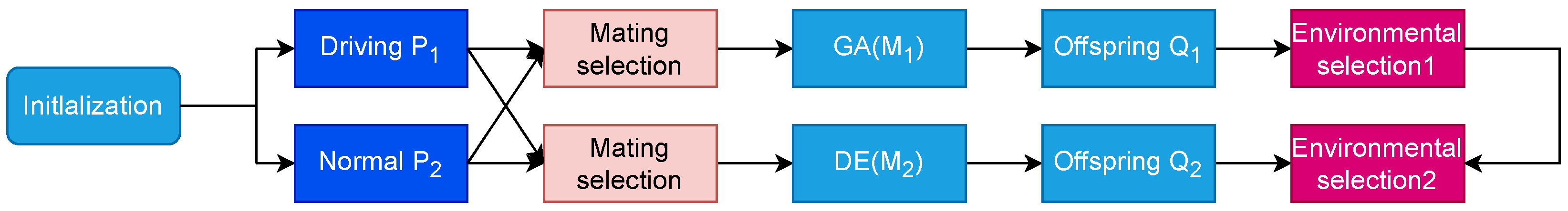
3.1. Framework of CMOEA-DCC

As illustrated in Figure 2, the CMOEA-DCC framework proposed in this paper incorporates two distinct populations: the driving population and the normal population. These two populations will iteratively undergo a series of evolutionary operations until the termination criteria are met. It is important to note that the evolutionary processes of the two populations are independent of each other, with interactions occurring only during the offspring generation phase. The role of the driving population is primarily manifested in its collaborative support to the normal population during the environmental selection phase. Furthermore, different environmental selection mechanisms are designed to cater to the characteristics of each population. The driving population focuses mainly on optimizing the objective function, thereby aiding solutions in traversing infeasible regions. Conversely, the normal population simultaneously considers both constraint conditions and the objective function during optimization, driving solutions to converge towards the boundaries of feasible regions.

According to the description in Algorithm 1, two populations are randomly generated in the initial phase. During the parent selection process, parent solutions are selected from the driving population $P_1$ and the normal population $P_2$ based on the probability value of $ratio$. The calculation formula for the probability value $ratio$ is as follows:

$$ratio=0.5\times \left(1-cos\left((1-fr)\pi \right)\right)$$

(4)

Algorithm 1 Framework of CMOEA-DCC

Input: N (population size) $ratio$ (probability parameter) a (balancing factor) Output: P (final population) 1:  $P_1\leftarrow$ Initialize the population (N); 2:  $P_2\leftarrow$ Initialize the population (N); 3:  while the terminal criterion is not fulfilled do 4:      $M_1\leftarrow$ Perform the elite mating selection ($P_1$, $P_2$, N, $ratio$); 5:      $Q_1\leftarrow$ Genetic operator($M_1$); 6:      $M_1\leftarrow$ Perform the elite mating selection ($P_1$, $P_2$, N, $ratio$); 7:      $Q_2\leftarrow$ DEgenerator($M_2$); 8:      $P_1\leftarrow$ EnvironmentalSelection1($P_1\cup Q_1$, N); 9:      $P_2\leftarrow$ EnvironmentalSelection2($P_1\cup P_2\cup Q_2$, N, a); 10: end while 11: $P\leftarrow$ final population; 12: Return P;

Subsequently, the driving population generates N offspring through a genetic algorithm $GA$, while the normal population produces N offspring using differential evolution. The combined GA/DE approach (Algorithm 1) achieves performance gains through synergistic advantage integration. The specific advantages are demonstrated as follows.

• Genetic Algorithm (GA) [40] Guided Population:

(1) Implements tournament selection and simulated binary crossover (SBX) crossover for global exploration;

(2) Maintains solution diversity via controlled parameterization ($p_c=0.9$, ${\eta }_c=15$);

(3) Preserves building blocks through selection pressure.

• Differential Evolution (DE) [41] Main Population:

(1) Adopts current-to-best/1 mutation for directed local search;

(2) Directional differential mutation accelerates convergence (exhibits rapid convergence toward the Pareto frontier);

(3) Optimized parameter settings ($F=0.5$, $CR=0.8$) balance exploration–exploitation.

Following this, the driving population and the normal population collaboratively perform environmental selection to filter out N high-quality solutions ($P_2$). The environmental selection for the driving population and the normal population follows the rules outlined in Algorithms 2 and Algorithm 3, respectively. Finally, the solutions from the last generation of the normal population are retained as the final population P.

Algorithm 2 EnvironmentalSelection1

Input: $P_1$ (driving population), $Q_1$(offspring population) Output: $P^{\prime }$ (new driving population) 1:  $U\leftarrow$$P_1\cup Q_1$; 2:  $Fitness\leftarrow$ The fitness values of the solutions in U are calculated using Formulas (5) and (6); 3:  $P_F\leftarrow$ Selection from U is performed based on the unconstrained non-dominated principle; 4:  $P_{F}sort\leftarrow$ Sort the $P_F$ in descending order based on fitness evaluation values; 5:  if  $P_F>N$  then 6:       Remove the lower-ranked redundant solutions based on the $P_{F}sort$; 7:  else 8:      The solutions in U are sorted based on their fitness values, and the top-ranked solutions are added to $P_F$; 9:  end if 10: $P^{\prime }\leftarrow$$P_F$; 11: Return $P^{\prime }$;

Algorithm 3 EnvironmentalSelection2

Input: $P^{\prime }$ (new driving population), $P_2$ (driving population), $Q_2$ (offspring population), a (balancing factor) Output: P (final population) 1: $U\leftarrow$ $P^{\prime }\cup P_2\cup Q_2$; 2: $R_O\leftarrow$ Layer the objectives function in U based on non-dominated sorting; 3: $R_O^i\leftarrow$ Sort the solutions in layer $R_O$ based on crowding distance; 4: $R_C\leftarrow$ Layer the constraints in U based on non-dominated sorting; 5: $R_C^i\leftarrow$ Sort the solutions in layer $R_C$ based on crowding distance; 6: Calculate the balance factor a using Equation (7); 7: Obtain the final ranking $R_r^i\left(t\right)$ through Equation (8); 8: $P\leftarrow$ Select the top N solutions in U based on the $R_r^i\left(t\right)$ ranking. 9: Return P;

3.2. Driving Population for Objectives

For the driving population, the calculation of fitness does not directly rely on the objective values of the solutions but instead determines the dominance relationship between solutions using the minimum SDE distance:

$$SDE\left(x\right)=\underset{y\in \mathcal{D}\left(x\right)}{min}\sqrt{\sum _{i=1}^m{(max\{0,f_i\left(y\right)-f_i\left(x\right)\})}^2}$$

(5)

Here, D represents the driving population, $f_i\left(x\right)$ denotes the i-th objective value of solution x, and m is the total number of objectives.

The minimum SDE distance is calculated by measuring the distance between solution x and other solutions in the objective space, which simultaneously evaluates both convergence and diversity, thereby filtering out higher-quality solutions. Subsequently, a fitness calculation method similar to that in SPEA2 [37] is employed:

$$fitness\left(x\right)=\sum _{y\in S_x,y\ne x}\left|R_y\right|+{\displaystyle \frac{1}{\mathrm{dist}(x,x^{\prime })+2}}$$

(6)

Here, $S_x$ represents the set of solutions that dominate solution x, and $R_y$ represents the set of solutions dominated by solution y. $x^{\prime }$ is the $\sqrt{2N}$-th nearest neighbor, and $\mathrm{dist}(x,x^{\prime })$ denotes the inverse of the Euclidean distance between solution x and $x^{\prime }$.

The environmental selection process for the driving population is detailed in Algorithm 2. As mentioned earlier, the fitness of solutions in the driving population is calculated using Formulas (3) and (4). After obtaining their fitness values, they are sorted in descending order to derive $P_{F}sort$. Subsequently, the front solutions are selected from the combined population U based on the unconstrained dominance principle. If the number of solutions in $P_F$ exceeds N, redundant solutions are removed according to their fitness values. If the number of solutions in $P_F$ is less than N, the solutions in U are sorted by their fitness values, and the top-ranked solutions are added to $P_F$ until N solutions are reached. Fitness evaluation is only used as a criterion for supplementing and removing redundant solutions in the driving population, aiming to ignore its constraints and promote faster convergence to the CPF.

3.3. Normal Population for Constraints

When evaluating individual performance, the performance measurement method must not only focus on the objective functions but also take into account the constraints, carefully considering the balance between the two. In this paper, to simplify the process, the Pareto optimality principle and constraint handling technique (CHT) are employed to evaluate individuals based on the objective functions and constraints, respectively.

Algorithm 3 details the steps for conventional population selection. Specifically, for each individual, the integrated population(U) is first sorted based on Pareto dominance and crowding distance to obtain a priority list (see lines 2–3 of Algorithm 3). Subsequently, the same population is sorted again using CDP combined with crowding distance to derive another priority list (see lines 4–5 of Algorithm 3). It is evident that the first sorting prioritizes the optimization level of the objective functions, while the second sorting places more emphasis on the satisfaction of constraints. In both ranking systems, a smaller value indicates the better overall performance of the individual. To balance the two priority lists, a dynamic balancing factor a is introduced, and its calculation formula is as follows:

$$a={sin}^2\left({\displaystyle \frac{\pi }{2}}·\left(1-{\displaystyle \frac{t}{\mathrm{T}}}\right)\right)$$

(7)

$$R_r^i\left(t\right)=a·R_O^1+(1-a)·R_C^1$$

(8)

Ultimately, the top N individuals with smaller $R_r^i\left(t\right)$ values are selected for the next generation population. It is evident that $R_r^i\left(t\right)$ prioritizes the objective functions in the early stages, thereby enhancing the global search capability across both feasible and infeasible regions. This aspect is particularly critical when addressing CMOPs with discontinuous feasible regions or those disrupted by infeasible areas. In practice, the regions explored during the initial phase lay a solid foundation for subsequent stages. In these later stages, the focus shifts to constraints by applying the CDP, thereby ensuring the identification of a feasible Pareto optimal solution set.

3.4. Complexity Analysis of CMOEA-DCC

In this section, we present a comprehensive complexity analysis of the proposed CMOEA-DCC, encompassing both time and space complexity.

3.4.1. Time Complexity

1.

Dual-population initialization: $\mathcal{O}\left(2N\right)\to \mathrm{Negligible}$

2.

Reproduction phase:

• Main population selection: $\mathcal{O}\left(M{N}^2\right)$
  textit (NSGA-III based mechanism)
• Auxiliary population selection: $\mathcal{O}(NlogN)$   (Simplified selection)

3.

Environmental selection:

• Non-dominated sorting: $\mathcal{O}\left(M{\left(2N\right)}^2\right)=\mathcal{O}\left(4M{N}^2\right)$
• Elitism preservation: $\mathcal{O}(NlogN)$

4.

Cooperative operation: $\mathcal{O}\left(MN\right)$   (Information exchange)

• Dominant term derivation:

$$\begin{array}{cc}\hfill T(M,N)& =\mathcal{O}\left(4M{N}^2\right)+\mathcal{O}\left(MN\right)+\mathcal{O}(NlogN)\hfill \\ \hfill & \approx \mathcal{O}\left(M{N}^2\right)(\mathrm{Preserving}\mathrm{highest}-\mathrm{order}\mathrm{term})\hfill \end{array}$$

3.4.2. Space Complexity

$$\begin{array}{cc}\hfill S(M,N)& =\underset{\mathrm{Dual}-\mathrm{population}\mathrm{storage}}{\underbrace{2N^2}}+\underset{\mathrm{Objective}\mathrm{matrix}}{\underbrace{MN}}+\underset{\mathrm{Distance}\mathrm{matrix}}{\underbrace{N^2}}\hfill \\ \hfill & +\underset{\mathrm{Elite}\mathrm{archive}}{\underbrace{N}}+\underset{\mathrm{Reference}\mathrm{points}}{\underbrace{M}}\hfill \end{array}$$

• Dominant term derivation:

$$\begin{array}{cc}\hfill S(M,N)& =\mathcal{O}\left(2N^2\right)+\mathcal{O}\left(MN\right)+\mathcal{O}\left(N^2\right)\hfill \\ \hfill & \approx \mathcal{O}\left(N^2\right)(\mathrm{when}N\gg M)\hfill \end{array}$$

4. Experimental Study

In this section, the proposed CMOEA-DCC is experimentally validated on two challenging benchmark test sets and real-world-case test sets, with seven state-of-the-art CMOEA algorithms selected as comparative counterparts. Subsequently, a series of experiments are conducted to evaluate the performance of CMOEA-DCC in handling various CMOPs, and a detailed analysis of the experimental results is provided. All experiments are executed on the PlatEMO [42] platform.

4.1. Experimental Setup

This section describes in detail the experimental setup designed to verify the effectiveness and performance of the proposed algorithm. The experimental configuration includes three key aspects: (1) test problem setup, (2) comparison algorithm setup, (3) performance index selection, and (4) termination parameter setup. These comprehensive settings not only lay a solid foundation for subsequent results but also ensure the integrity and reliability of CMOEA-DCC theoretical verification.

4.1.1. Test Problem Setup

To evaluate the performance of CMOEA-DCC across various test problems, this paper selects two representative benchmark test sets, encompassing 28 recently proposed CMOPs (such as MW1-14 [43] and LIRCMOP1-14 [44]). These problems have significantly varying feasible regions, posing a considerable challenge to CMOEA algorithms. Among them, MW4, MW8, MW14, LIRCMOP13, and LIRCMOP14 have three objective functions, while the remaining CMOPs have two objective functions, with the number of decision variables uniformly set to 10 to ensure the effective convergence of most CMOEAs. Additionally, five real-world case problems were selected for comparison experiments to verify the applicability of CMOEA-DCC.

4.1.2. Algorithm Setup

The algorithms parameters of the algorithms were tuned based on the recommendations provided in their original papers. For example, population sizes, crossover probabilities, mutation rates, and other algorithm-specific parameters were adjusted to align with best practices in the field. Where applicable, we employed empirical optimization methods to fine-tune key parameters, ensuring the best balance between exploration and exploitation during the optimization process. For example, we conducted preliminary tests on different population sizes and mutation rates to determine the optimal configuration for each algorithm. This study selects seven state-of-the-art CMOEAs (i.e., NSGAIII [45], ANSGAIII [46], BiCo [47], POCEA [48], ToP [26], TiGE2 [30], and CMOEMT [49]) as comparative algorithms. These algorithms are chosen as representative methods due to their outstanding performance in recent years.

Population size: The population size was set to 100 for all algorithms in the experiment. The population size follows standard settings in the multi-objective optimization field.

Genetic operator: In the experiment, the ToP algorithm uses simulated binary crossover ($SBX$) and polynomial mutation ($PM$) to generate offspring, where the crossover probability is set to 1 and the mutation probability is set to $1/D$ (D represents the problem dimension). A differential evolution algorithm is used to generate offspring. The parameter configurations for all comparative algorithms are set according to the recommended values in their original papers.

4.1.3. Performance Index Selection

This paper employs two of the most commonly used metrics, namely, IGD+ and HV. Specifically, a lower IGD+ value indicates better algorithm performance and vice versa. A higher HV value indicates better algorithm performance, whereas a lower value suggests poorer algorithm performance. In the table, “+”, “−”, and ”≈” denote that the compared CMOEA performs significantly better, significantly worse, or shows no significant difference compared to CMOEA-DCC, respectively. The gray-highlighted data in the table indicate the best values obtained.

4.1.4. Termination Parameter Setup

It is worth noting that, since the algorithm involves two populations, stopping conditions based on the same number of iterations or generations may lead to unfair comparisons. To ensure the fairness of the experiments, the total number of function evaluations is uniformly set to 200,000, and the calculation of the number of function evaluations includes all fitness evaluations from the driving population and normal population. Additionally, each algorithm is independently run 20 times on every CMOP.

4.2. Experimental Results on the MW Test Set

Table 1. The IGD+ results (mean and standard deviation) obtained by eight algorithms on the MW test suite.

Problem	M	D	NSGAIII	ANSGAIII	BiCo	POCEA	ToP	TiGE2	CMOEMT	CMOEA-DCC
MW1	2	15	2.3212e-3 (9.25e-5) −	4.4150e-3 (1.01e-2) −	1.6124e-3 (1.10e-5) ≈	7.0246e-3 (9.94e-4) −	NaN (NaN)	1.4272e-2 (9.03e-3) −	9.0638e-2 (4.42e-2) −	1.6166e-3 (1.06e-5)
MW2	2	15	2.3363e-2 (9.53e-3) −	2.0643e-2 (6.39e-3) −	1.1374e-2 (7.98e-3) ≈	1.1063e-1 (6.98e-2) −	1.3611e-1 (9.35e-2) −	6.6549e-1 (5.34e-2) −	4.0501e-2 (2.85e-2) −	4.4367e-3 (2.12e-3)
MW3	2	15	4.5330e-3 (5.57e-4) +	9.8468e-2 (2.81e-1) −	4.6843e-3 (2.11e-4) ≈	1.0727e-2 (1.78e-3) −	5.1955e-1 (4.60e-1) −	2.2084e-2 (4.22e-3) −	1.6305e-2 (3.24e-3) −	4.5787e-3 (1.10e-4)
MW4	3	15	4.1178e-2 (7.43e-5) +	4.1238e-2 (2.06e-4) +	4.1058e-2 (4.99e-4) +	5.0664e-2 (1.69e-3) −	3.9785e-1 (0.00e+0) ≈	1.2044e-1 (4.70e-2) −	1.1079e-1 (2.35e-2) −	4.1623e-2 (3.12e-4)
MW5	2	15	1.5977e-1 (2.67e-1) −	1.2875e-1 (2.67e-1) −	5.3010e-4 (4.13e-4) −	6.5924e-2 (1.09e-2) −	7.3984e-1 (9.13e-3) −	3.5717e-2 (7.75e-3) −	7.7276e-2 (2.06e-2) −	1.2564e-4 (5.54e-5)
MW6	2	15	2.6555e-2 (2.84e-2) −	2.6745e-2 (1.26e-2) −	8.8604e-3 (6.57e-3) −	4.9280e-1 (3.38e-1) −	5.1175e-1 (3.59e-1) −	2.7585e-1 (3.37e-1) −	3.6539e-2 (1.27e-2) −	3.8251e-3 (2.22e-3)
MW7	2	15	2.9207e-2 (1.00e-1) ≈	4.9102e-2 (1.38e-1) ≈	4.2519e-3 (2.13e-4) +	1.2949e-2 (1.66e-3) −	1.3725e-2 (2.56e-3) −	4.6804e-2 (2.38e-2) −	1.5659e-2 (3.63e-3) −	4.4269e-3 (2.96e-4)
MW8	3	15	5.4555e-2 (8.83e-3) −	1.1527e-1 (1.62e-1) −	4.5475e-2 (1.28e-3) −	1.0552e-1 (4.53e-2) −	4.1192e-1 (3.80e-1) −	6.8180e-1 (1.21e-1) −	7.0693e-2 (2.33e-2) −	4.3093e-2 (6.81e-4)
MW9	2	15	6.7893e-3 (2.08e-3) −	9.2317e-3 (3.51e-3) −	4.7970e-3 (5.29e-4) −	3.2400e-2 (5.90e-3) −	6.7423e-1 (1.21e-1) −	1.0892e-1 (1.79e-1) −	9.5902e-2 (2.11e-1) −	4.2306e-3 (1.78e-4)
MW10	2	15	1.7397e-1 (1.77e-1) −	1.6006e-1 (1.84e-1) −	1.0895e-1 (7.02e-2) −	4.4117e-1 (2.14e-1) −	NaN (NaN)	6.2359e-2 (5.25e-2) −	8.3408e-2 (5.89e-2) −	5.3724e-3 (3.81e-3)
MW11	2	15	4.8952e-1 (3.23e-1) −	3.8765e-1 (3.51e-1) −	5.9494e-3 (9.42e-5) ≈	3.4567e-2 (7.99e-3) −	3.2681e-1 (3.03e-1) −	3.8798e-2 (1.12e-2) −	1.8706e-2 (4.97e-3) −	5.9309e-3 (1.20e-4)
MW12	2	15	4.6820e-3 (1.13e-5) −	6.8828e-3 (8.43e-4) −	4.6327e-3 (8.08e-5) ≈	1.4905e-2 (1.50e-3) −	6.1013e-1 (3.03e-1) −	7.4271e-2 (1.70e-1) −	2.6368e-2 (1.05e-2) −	4.6022e-3 (8.54e-5)
MW13	2	15	1.1180e-1 (5.55e-2) −	2.4613e-1 (4.18e-1) −	4.4936e-2 (2.32e-2) −	3.0126e-1 (2.39e-1) −	6.3788e-1 (4.32e-1) −	1.1183e+0 (6.09e-1) −	1.0459e-1 (3.46e-2) −	1.1911e-2 (3.83e-3)
MW14	3	15	1.3056e-1 (3.48e-3) −	1.1180e-1 (2.46e-3) −	9.8229e-2 (1.72e-3) −	1.4401e-1 (2.57e-3) −	2.0966e-1 (1.19e-1) −	1.5536e-1 (7.73e-3) −	7.1254e-1 (1.98e-1) −	9.6813e-2 (1.49e-3)
$+/-/\approx$			2/11/1	1/12/1	2/7/5	0/14/0	0/11/1	0/14/0	0/14/0

and

Table 2. The HV results (mean and standard deviation) obtained by eight algorithms on the MW test suite.

Problem	M	D	NSGAIII	ANSGAIII	BiCo	POCEA	ToP	TiGE2	CMOEMT	CMOEA-DCC
MW1	2	15	4.8889e-1 (1.03e-4) −	4.8651e-1 (1.14e-2) −	4.9013e-1 (1.16e-5) +	4.7943e-1 (2.22e-3) −	NaN (NaN)	4.7444e-1 (1.07e-2) −	3.7795e-1 (3.83e-2) −	4.9008e-1 (2.46e-5)
MW2	2	15	5.4918e-1 (1.54e-2) −	5.5304e-1 (1.05e-2) −	5.6915e-1 (1.37e-2) ≈	4.3168e-1 (8.12e-2) −	4.0779e-1 (1.04e-1) −	1.0922e-1 (3.50e-2) −	5.2371e-1 (3.92e-2) −	5.8116e-1 (3.52e-3)
MW3	2	15	5.4558e-1 (5.12e-4) +	4.9005e-1 (1.68e-1) −	5.4454e-1 (4.14e-4) −	5.3702e-1 (2.51e-3) −	2.3056e-1 (2.65e-1) −	5.3090e-1 (2.80e-3) −	5.2490e-1 (6.74e-3) −	5.4485e-1 (2.31e-4)
MW4	3	15	8.4165e-1 (7.56e-5) +	8.4161e-1 (1.82e-4) +	8.4141e-1 (5.79e-4) +	8.2883e-1 (2.30e-3) −	3.2969e-1 (0.00e+0) ≈	7.5531e-1 (4.83e-2) −	7.4032e-1 (3.39e-2) −	8.4026e-1 (5.93e-4)
MW5	2	15	2.6208e-1 (8.69e-2) −	2.7718e-1 (8.34e-2) −	3.2437e-1 (2.84e-4) −	2.6713e-1 (1.32e-2) −	8.0254e-2 (1.49e-2) −	3.0752e-1 (3.67e-3) −	2.3863e-1 (2.70e-2) −	3.2468e-1 (4.25e-5)
MW6	2	15	2.9588e-1 (2.80e-2) −	2.9282e-1 (1.70e-2) −	3.1887e-1 (9.94e-3) −	1.2047e-1 (1.08e-1) −	1.2239e-1 (1.03e-1) −	2.1019e-1 (8.33e-2) −	2.7929e-1 (1.85e-2) −	3.2658e-1 (4.01e-3)
MW7	2	15	4.0355e-1 (3.73e-2) ≈	3.9563e-1 (5.16e-2) ≈	4.1243e-1 (3.38e-4) +	4.0277e-1 (2.09e-3) −	3.9828e-1 (3.04e-3) −	3.8952e-1 (6.62e-3) −	3.9896e-1 (4.10e-3) −	4.1220e-1 (3.01e-4)
MW8	3	15	5.1697e-1 (2.60e-2) −	4.8767e-1 (8.58e-2) −	5.3962e-1 (8.47e-3) −	4.0894e-1 (8.13e-2) −	2.5921e-1 (1.79e-1) −	1.4376e-1 (3.83e-2) −	4.7820e-1 (4.53e-2) −	5.4899e-1 (4.46e-3)
MW9	2	15	3.9269e-1 (3.98e-3) −	3.8913e-1 (5.54e-3) −	3.9639e-1 (2.59e-3) −	3.5241e-1 (5.60e-3) −	1.9241e-2 (5.51e-2) −	3.3198e-1 (8.37e-2) −	3.2620e-1 (7.81e-2) −	3.9868e-1 (1.56e-3)
MW10	2	15	3.3799e-1 (8.67e-2) −	3.4706e-1 (9.09e-2) −	3.7032e-1 (3.84e-2) −	2.0323e-1 (9.70e-2) −	NaN (NaN)	3.9939e-1 (3.48e-2) −	3.8526e-1 (3.58e-2) −	4.5141e-1 (6.41e-3)
MW11	2	15	3.2492e-1 (8.17e-2) −	3.5067e-1 (8.89e-2) −	4.4809e-1 (1.44e-4) +	4.3016e-1 (4.27e-3) −	3.5821e-1 (7.57e-2) −	4.3324e-1 (3.08e-3) −	4.4071e-1 (1.88e-3) −	4.4791e-1 (1.35e-4)
MW12	2	15	6.0511e-1 (5.24e-5) −	6.0233e-1 (8.74e-4) −	6.0530e-1 (1.54e-4) ≈	5.9053e-1 (2.14e-3) −	1.1708e-1 (2.06e-1) −	5.4589e-1 (1.29e-1) −	5.7818e-1 (1.60e-2) −	6.0525e-1 (1.24e-4)
MW13	2	15	4.2671e-1 (2.65e-2) −	3.9971e-1 (7.43e-2) −	4.5797e-1 (1.00e-2) −	3.1855e-1 (9.45e-2) −	2.4748e-1 (1.19e-1) −	2.1659e-1 (9.83e-2) −	4.3310e-1 (1.60e-2) −	4.7577e-1 (3.63e-3)
MW14	3	15	4.6598e-1 (1.53e-3) −	4.7006e-1 (1.69e-3) −	4.6985e-1 (1.30e-3) −	4.5098e-1 (3.77e-3) −	4.1457e-1 (5.45e-2) −	4.5133e-1 (4.78e-3) −	2.2506e-1 (7.75e-2) −	4.7132e-1 (1.65e-3)
$+/-/\approx$			2/11/1	1/12/1	4/8/2	0/14/0	0/11/1	0/14/0	0/14/0

present the IGD+ and HV values of the proposed CMOEA-DCC algorithm and other compared algorithms on the constrained MW test suite.

As shown in Table 1, CMOEA-DCC achieves the best results on seven CMOPs, while NSGAIII, NSGAIII, and BiCo obtain the best results on two, one, and two problems, respectively. ToP, TiGE2, POCEA, and CMOEMT however, do not achieve any best results. Additionally, CMOEA-DCC significantly outperforms NSGAIII, ANSGAIII, BiCo, POCEA, ToP, TiGE2, and CMOEMT on 11, 12, 7, 14, 11, 14, and 14 test problems, respectively. From Table 1, it can be observed that CMOEA-DCC did not achieve the best values when dealing with discontinuous feasible regions, such as in MW1 and MW3. Compared to the MW3 test problem, NSGA-III demonstrated strong capability in handling it and obtained the best values. For the three-objective MW4 test problem and the continuous MW7 test problem, BiCo achieved the best results. This indirectly indicates that CMOEA-DCC still has significant room for improvement in handling multi-objective and simple continuous test problems.

Table 2 shows that CMOEA-DCC achieves the best results on eight CMOPs, further demonstrating its competitiveness. The seven compared algorithms underperform on multiple problems, once again validating the superiority of CMOEA-DCC. NSGA-III achieved the best values on the MW3 and MW4 test problems, while BiCo obtained the best results on MW1, MW4, MW11, and MW12. This once again demonstrates that CMOEA-DCC exhibits strong capability in handling narrow and discontinuous test problems but lacks targeted optimization for simpler discontinuous cases. Overall, although CMOEA-DCC performs suboptimally on a few problems, it significantly outperforms the other algorithms in general.

To further analyze the differences in solution distribution between CMOEA-DCC and competing algorithms, we present the solution distributions of eight CMOEAs on the MW13 test problem. As shown in Figure 3, only some solutions of POCEA, ToP, and TiGE2 are distributed on the PF, primarily due to their limited exploration capabilities, which prevent some solutions from locating the PF. Although all solutions of NSGAIII, BiCo, ANSGAIII, and CMOEMT lie on the PF, their distributions are sparse and uneven, mainly because they fail to balance diversity and convergence. In contrast, the solutions of CMOEA-DCC not only all lie on the PF but are also densely and uniformly distributed, further demonstrating its superiority.

The variance data in parentheses in Table 1 and Table 2 demonstrate the stability and robustness of the algorithms. Clearly, CMOEA-DCC achieves outstanding performance on most test problems. Furthermore, the PF comparative experiments in Figure 3 show that CMOEA-DCC produces not only uniformly but also densely distributed solutions, which further confirms its strong stability and excellent robustness.

4.3. Experimental Results on the LIRCMOP Test Set

We aimed to develop a multiple comparisons test (Friedman test) for statistical analysis on the LIRCMOP test suite.

Table 3. The IGD+ results (mean and standard deviation) obtained by eight algorithms on the LIR-CMOP test suite.

Problem	M	D	NSGAIII	ANSGAIII	BiCo	POCEA	ToP	TiGE2	CMOEMT	CMOEA-DCC
LIRCMOP1	2	30	3.1107e-1 (3.01e-2) −	2.9308e-1 (3.81e-2) −	1.9127e-1 (1.23e-2) ≈	4.9416e-2 (1.34e-2) ≈	3.1795e-1 (1.82e-2) −	2.1528e-1 (2.33e-2) ≈	3.3986e-1 (1.69e-2) −	1.4497e-1 (8.40e-2)
LIRCMOP2	2	30	2.6063e-1 (1.62e-2) −	2.5803e-1 (2.75e-2) −	1.5915e-1 (1.57e-2) ≈	5.4916e-2 (1.87e-2) ≈	2.7320e-1 (1.63e-2) −	1.9342e-1 (1.44e-2) ≈	2.7467e-1 (3.39e-2) −	1.2849e-1 (6.51e-2)
LIRCMOP3	2	30	3.1511e-1 (2.94e-2) −	3.0279e-1 (4.69e-2) −	1.9590e-1 (2.27e-2) −	1.7752e-1 (1.30e-1) ≈	3.4453e-1 (2.39e-2) −	2.1528e-1 (1.73e-2) ≈	2.9253e-1 (4.21e-2) −	1.7994e-1 (9.04e-2)
LIRCMOP4	2	30	2.8466e-1 (2.88e-2) −	2.8403e-1 (3.00e-2) −	1.9436e-1 (2.49e-2) ≈	1.6376e-1 (1.13e-1) ≈	3.1396e-1 (1.11e-2) −	2.1389e-1 (1.96e-2) ≈	2.8009e-1 (3.38e-2) −	1.7744e-1 (7.95e-2)
LIRCMOP5	2	30	1.2237e+0 (5.18e-3) −	1.2256e+0 (8.14e-3) −	1.2186e+0 (6.32e-3) −	7.0890e-1 (7.31e-1) ≈	1.1616e+0 (8.89e-2) ≈	8.2943e-1 (4.40e-1) ≈	1.3044e+0 (1.84e-1) −	8.4148e-1 (5.57e-1)
LIRCMOP6	2	30	1.3459e+0 (3.88e-4) −	1.3459e+0 (3.83e-4) −	1.3452e+0 (1.32e-4) ≈	9.7138e-1 (5.31e-1) −	1.2085e+0 (3.37e-1) −	1.2223e+0 (3.34e-1) −	1.3602e+0 (1.47e-2) −	6.9698e-1 (5.22e-1)
LIRCMOP7	2	30	3.6777e-1 (5.68e-1) ≈	5.3372e-1 (6.81e-1) −	3.6153e-1 (5.69e-1) ≈	6.1252e-1 (7.24e-1) −	9.0243e-1 (8.07e-1) −	3.1710e-1 (1.72e-1) −	1.0872e+0 (6.90e-1) −	8.4017e-2 (4.34e-2)
LIRCMOP8	2	30	8.1133e-1 (7.30e-1) −	1.1782e+0 (7.05e-1) −	1.3412e+0 (6.13e-1) −	5.9914e-1 (6.47e-1) −	1.2653e+0 (6.66e-1) −	4.9222e-1 (3.34e-1) −	1.3836e+0 (5.53e-1) −	4.2964e-2 (3.49e-2)
LIRCMOP9	2	30	9.4277e-1 (1.36e-1) −	9.9285e-1 (7.34e-2) −	9.0201e-1 (1.55e-1) −	6.2461e-1 (1.11e-1) ≈	5.4575e-1 (1.24e-1) ≈	8.1640e-1 (2.03e-1) −	1.0183e+0 (1.42e-1) −	2.2846e-1 (1.64e-1)
LIRCMOP10	2	30	8.3578e-1 (9.81e-2) −	8.7389e-1 (9.36e-2) −	8.8950e-1 (4.46e-2) −	4.1322e-1 (3.02e-1) ≈	3.9541e-1 (9.97e-2) ≈	9.9579e-1 (1.62e-1) −	1.0074e+0 (9.14e-2) −	6.5313e-2 (9.10e-2)
LIRCMOP11	2	30	7.2783e-1 (1.08e-1) −	7.2036e-1 (1.14e-1) −	4.5439e-1 (1.98e-1) −	4.5300e-1 (2.63e-1) −	3.5124e-1 (9.28e-2) ≈	9.4417e-1 (3.52e-1) −	9.3467e-1 (1.50e-1) −	3.5339e-2 (4.16e-2)
LIRCMOP12	2	30	7.4681e-1 (1.73e-1) −	8.0294e-1 (1.44e-1) −	3.2114e-1 (1.42e-1) ≈	3.2182e-1 (8.02e-2) ≈	2.7020e-1 (7.86e-2) ≈	4.6064e-1 (1.00e-1) −	8.7013e-1 (2.83e-1) −	1.6658e-1 (8.32e-2)
LIRCMOP13	3	30	1.3026e+0 (2.40e-4) −	1.3166e+0 (3.89e-3) −	1.2575e+0 (2.74e-1) −	4.2133e-1 (5.53e-1) ≈	1.2965e+0 (1.25e-1) −	1.2487e+0 (3.21e-1) −	2.7971e-1 (2.22e-2) ≈	1.0342e-1 (2.26e-3)
LIRCMOP14	3	30	1.2591e+0 (1.12e-3) −	1.2725e+0 (5.01e-3) −	1.2751e+0 (1.60e-3) −	2.2822e-1 (3.70e-1) ≈	1.2328e+0 (1.50e-1) −	1.1247e+0 (3.82e-1) −	2.4478e-1 (1.47e-2) ≈	9.7563e-2 (9.56e-4)
$+/-/\approx$			0/13/1	0/14/0	0/8/6	0/4/10	0/9/5	0/9/5	0/12/2

presents the IGD+ values of the CMOEA-DCC algorithm and other compared algorithms on the constrained LIRCMOP test suite. CMOEA-DCC achieved the best results on eight CMOPs, while its competitor POCEA only attained the best values on two test problems. Additionally, CMOEA-DCC significantly outperforms NSGAIII, ANSGAIII, BiCo, POCEA, ToP, TiGE2, and CMOEMT on 13, 14, 8, 4, 9, 9, and 12 test problems, respectively.

Table 4. The HV results (mean and standard deviation) obtained by eight algorithms on the LIR-CMOP test suite.

Problem	M	D	NSGAIII	ANSGAIII	BiCo	POCEA	ToP	TiGE2	CMOEMT	CMOEA-DCC
LIRCMOP1	2	30	1.0980e-1 (9.49e-3) −	1.1679e-1 (1.12e-2) −	1.4808e-1 (5.60e-3) ≈	2.0910e-1 (6.31e-3) ≈	1.1129e-1 (7.87e-3) −	1.3830e-1 (1.03e-2) ≈	1.0091e-1 (4.59e-3) −	1.7354e-1 (3.62e-2)
LIRCMOP2	2	30	2.2568e-1 (7.94e-3) −	2.2991e-1 (1.51e-2) −	2.7185e-1 (9.50e-3) ≈	3.3364e-1 (7.37e-3) ≈	2.2230e-1 (1.15e-2) −	2.6280e-1 (8.07e-3) ≈	2.1985e-1 (1.55e-2) −	2.9473e-1 (3.32e-2)
LIRCMOP3	2	30	9.8499e-2 (8.88e-3) −	1.0600e-1 (1.30e-2) −	1.3194e-1 (8.30e-3) ≈	1.3970e-1 (3.71e-2) ≈	9.2775e-2 (4.48e-3) −	1.2741e-1 (6.68e-3) ≈	1.0345e-1 (1.17e-2) −	1.3925e-1 (2.88e-2)
LIRCMOP4	2	30	1.9554e-1 (1.29e-2) −	1.9629e-1 (1.44e-2) −	2.3045e-1 (1.22e-2) ≈	2.4561e-1 (3.48e-2) ≈	1.8327e-1 (1.07e-2) −	2.2401e-1 (1.04e-2) ≈	1.9454e-1 (1.38e-2) −	2.4479e-1 (3.38e-2)
LIRCMOP5	2	30	0.0000e+0 (0.00e+0) ≈	0.0000e+0 (0.00e+0) ≈	0.0000e+0 (0.00e+0) ≈	1.3653e-1 (1.40e-1) ≈	1.7902e-3 (8.01e-3) ≈	6.2636e-2 (7.20e-2) ≈	0.0000e+0 (0.00e+0) ≈	8.6415e-2 (1.35e-1)
LIRCMOP6	2	30	0.0000e+0 (0.00e+0) −	0.0000e+0 (0.00e+0) −	0.0000e+0 (0.00e+0) −	4.9125e-2 (6.88e-2) ≈	8.6248e-3 (2.11e-2) −	1.3063e-2 (3.19e-2) −	0.0000e+0 (0.00e+0) −	7.7071e-2 (7.19e-2)
LIRCMOP7	2	30	2.0713e-1 (8.97e-2) ≈	1.7913e-1 (1.06e-1) −	2.0836e-1 (9.01e-2) ≈	1.6747e-1 (1.13e-1) −	1.3096e-1 (1.36e-1) −	2.0490e-1 (2.84e-2) −	8.6706e-2 (1.00e-1) −	2.6179e-1 (1.68e-2)
LIRCMOP8	2	30	1.3362e-1 (1.12e-1) −	7.7394e-2 (1.08e-1) −	4.9009e-2 (9.14e-2) −	1.6601e-1 (9.84e-2) −	7.1067e-2 (1.14e-1) −	1.7317e-1 (4.94e-2) −	4.2404e-2 (7.75e-2) −	2.7820e-1 (1.50e-2)
LIRCMOP9	2	30	1.3240e-1 (6.48e-2) −	1.0870e-1 (3.57e-2) −	1.5948e-1 (8.23e-2) −	2.9007e-1 (6.35e-2) ≈	3.2885e-1 (8.17e-2) ≈	2.0966e-1 (8.15e-2) −	1.1293e-1 (6.34e-2) −	4.9342e-1 (6.49e-2)
LIRCMOP10	2	30	1.1869e-1 (8.21e-2) −	9.5717e-2 (4.61e-2) −	8.6704e-2 (2.20e-2) −	4.2876e-1 (1.99e-1) ≈	4.9376e-1 (8.28e-2) ≈	1.3918e-1 (9.25e-2) −	7.3399e-2 (2.80e-2) −	6.7830e-1 (4.27e-2)
LIRCMOP11	2	30	2.4692e-1 (7.59e-2) −	2.4286e-1 (6.75e-2) −	4.0824e-1 (1.27e-1) −	4.1752e-1 (1.48e-1) −	4.6207e-1 (7.44e-2) ≈	1.7274e-1 (9.95e-2) −	1.7346e-1 (7.21e-2) −	6.7669e-1 (2.37e-2)
LIRCMOP12	2	30	2.8904e-1 (9.71e-2) −	2.4960e-1 (8.20e-2) −	4.7732e-1 (6.08e-2) ≈	4.5409e-1 (4.77e-2) ≈	4.8963e-1 (4.24e-2) ≈	3.7467e-1 (5.94e-2) −	2.2078e-1 (1.02e-1) −	5.4108e-1 (4.39e-2)
LIRCMOP13	3	30	4.4509e-4 (7.87e-6) −	2.8904e-4 (1.43e-4) −	2.7747e-2 (1.24e-1) −	4.0214e-1 (2.39e-1) ≈	9.2131e-3 (2.25e-2) −	3.2273e-2 (8.07e-2) −	3.6032e-1 (1.87e-2) ≈	5.3477e-1 (3.31e-3)
LIRCMOP14	3	30	9.6071e-4 (1.26e-4) −	7.0184e-4 (2.83e-4) −	4.0281e-4 (2.52e-4) −	4.8583e-1 (1.66e-1) ≈	1.6602e-2 (3.43e-2) −	6.9573e-2 (1.19e-1) −	4.0060e-1 (1.50e-2) ≈	5.4964e-1 (1.52e-3)
$+/-/\approx$			0/12/2	0/13/1	0/7/7	0/3/11	0/9/5	0/9/5	0/11/3

shows the HV values of the eight algorithms, with CMOEA-DCC again achieving the best results on nine CMOPs, further demonstrating its competitiveness. The seven compared algorithms underperform on 12, 13, 7, 3, 9, 9, and 11 problems, respectively, once again validating the superiority of CMOEA-DCC. Overall, although CMOEA-DCC performs slightly worse on a few problems, it significantly outperforms the other algorithms in general.

As clearly shown in Table 3 and Table 4, POCEA outperforms CMOEA-DCC on the LIRCMOP1 and LIRCMOP2 test problems. This further demonstrates that CMOEA-DCC’s dual-population collaboration approach fails to achieve the best constrained Pareto front when dealing with simple and discontinuous feasible regions. These results indicate that while CMOEA-DCC excels at handling complex, narrow, and multi-objective-conflicting feasible regions, it does not deliver optimal results for simpler Pareto fronts.

To further validate the superiority of CMOEA-DCC, Figure 4 presents the PF plots of eight algorithms on LIRCMOP14. It is clear that NSGAIII, ANSGAIII, BiCo, ToP, and TiGE2 fail to locate the true PF, with all solutions even failing to reach the feasible region, indicating poor exploration capabilities of these algorithms, which significantly degrades their performance. Although most solutions of CMOEMT and POCEA locate the PF, they are not uniformly distributed on the PF, primarily due to the inability to balance constraint satisfaction and objective conflicts. In contrast, CMOEA-DCC has only one solution not on the PF, while all others are not only uniformly distributed on the PF but also densely concentrated, further demonstrating that CMOEA-DCC outperforms its competitors.

From the robustness analysis (the variance data in parentheses in Table 3 and Table 4) of the algorithm, CMOEA-DCC achieves remarkable performance in complex and narrow feasible regions. This is primarily attributed to the collaborative cooperation of its dual populations, which effectively balances diversity and convergence, thereby providing stable fluctuation space. As evidenced by the comparative experimental results of LIRCMOP14 in Figure 4, CMOEA-DCC demonstrates more concentrated and uniform distribution compared to the seven competing algorithms, further validating its strong robustness.

4.4. Performance Analysis

Table 5. Results obtained by the Wilcoxon test for algorithm CMOEA-DCC.

CMOEA-DCC vs.	IGD			HV
	${\mathit{R}}^{+}$	${\mathit{R}}^{-}$	p-Value	${\mathit{R}}^{+}$	${\mathit{R}}^{-}$	p-Value
NSGAIII	402.0	4.0	0.000006	373.5	4.5	0.000008
ANSGAIII	405.0	1.0	0.000004	404.0	2.0	0.000004
BiCo	393.0	13.0	0.000014	367.0	11.0	0.000014
POCEA	354.0	52.0	0.000561	366.0	40.0	0.000181
ToP	406.0	0.0	0.000004	378.0	−1.0	0.000003
TiGE2	405.0	1.0	0.000004	406.0	0.0	0.000004
CMOEMT	406.0	0.0	0.000004	406.0	0.0	0.000004

presents the results of the Wilcoxon rank-sum test comparing CMOEA-DCC with seven other algorithms. The values $R^{+}$, $R^{-}$, and p-value denote cases where CMOEA-DCC performs better, worse, or similarly, respectively. For the IGD metric, POCEA exhibited the highest $R^{-}$ value at 52.0, while in terms of HV, POCEA again had the highest $R^{-}$ value of 40.0. In contrast, CMOEA-DCC consistently obtained significantly higher $R^{+}$ values across both IGD and HV, with the lowest values reaching 354.0 and 366.0, and the highest up to 406.0. These results clearly demonstrate that CMOEA-DCC delivers superior overall performance compared to the other algorithms.

4.5. Experimental Results on the Real-World Case Problems

To further validate the applicability of CMOEA-DCC in real-world problems [50,51], we selected five common real-world problems (vibrating platform [52], two-bar truss design [2], disc brake design [28], gear train design [23], and car side-impact design [22]) as comparison objects for seven competing algorithms and CMOEA-DCC.

Since the competing algorithms do not have a true PF in real-world problems, we only use their HV values as the comparison metric. As shown in

Table 6. The HV results (mean and standard deviation) obtained by eight algorithms on the real-world case problems.

Problem	M	D	NSGAIII	ANSGAIII	BiCo	POCEA	ToP	TiGE2	CMOEMT	CMOEA-DCC
VPF	2	5	3.6852e-1 (7.57e-2) −	3.8214e-1 (3.69e-2) −	3.8162e-1 (3.10e-2) −	1.4585e-1 (1.17e-1) −	3.9295e-1 (1.29e-5) −	2.3649e-1 (1.73e-1) −	3.9290e-1 (4.15e-5) −	3.9301e-1 (6.77e-6)
TBTD	2	3	8.9418e-1 (2.07e-3) −	8.9395e-1 (1.91e-3) −	8.9999e-1 (3.29e-4) −	3.7923e-1 (2.60e-1) −	9.0207e-1 (1.33e-4) −	8.9517e-1 (1.61e-3) −	8.9847e-1 (6.65e-4) −	9.0249e-1 (1.15e-4)
DBD	2	4	4.3457e-1 (9.84e-4) −	4.2563e-1 (7.56e-3) −	4.3495e-1 (9.21e-5) −	4.2550e-1 (1.65e-3) −	4.3451e-1 (1.63e-4) −	4.1468e-1 (4.65e-3) −	4.3450e-1 (1.68e-4) −	4.3516e-1 (8.30e-5)
GTD	2	4	4.8474e-1 (1.87e-4) +	4.8394e-1 (5.68e-4) −	4.8461e-1 (3.03e-5) −	4.8107e-1 (9.50e-4) −	4.8444e-1 (5.35e-5) −	4.0931e-1 (2.75e-2) −	4.8461e-1 (3.55e-5) −	4.8470e-1 (3.86e-5)
CSID	3	7	2.5506e-2 (1.69e-4) −	2.5595e-2 (1.28e-4) −	2.6144e-2 (3.28e-5) ≈	2.2555e-2 (1.69e-3) −	2.5705e-2 (9.76e-5) −	2.0399e-2 (1.25e-4) −	2.5863e-2 (5.83e-5) −	2.6148e-2 (3.31e-5)
$+/-/\approx$			1/4/0	0/5/0	0/4/1	0/5/0	0/5/0	0/5/0	0/5/0

, we can observe the HV values of the seven competing algorithms and CMOEA-DCC. CMOEA-DCC achieves the best results on all four real-world test problems, with only NSGAIII attaining the optimal value on GTD, fully demonstrating the strong applicability of CMOEA-DCC in real-world scenarios.

5. Conclusions

This paper proposes a CMOEA-DCC algorithm for solving CMOPs, which operates through the collaborative functioning of a driving population and a normal population. In the driving population, the algorithm focuses on objective optimization to help solutions cross infeasible regions and utilizes the minimum SDE distance in environmental selection to enhance the convergence and diversity of solutions. The normal population places more emphasis on constraint conditions, ensuring that solutions remain within feasible regions while balancing objectives and constraints. Additionally, the driving population and the normal population collaborate in environmental selection to retain solutions with good convergence and diversity.

In the experimental section, CMOEA-DCC was evaluated on 28 CMOPs from two benchmark suites and five representative real-world cases, with comparisons made against seven state-of-the-art CMOEAs to validate its effectiveness. The experimental results demonstrate that while CMOEA-DCC achieved optimal values and outperformed competing algorithms on most test problems, it failed to obtain the best CPF when handling simple feasible regions. This further indicates that CMOEA-DCC’s focus on addressing complex, narrow, and multi-objective feasible regions led to its neglect of simpler cases, which represents an important direction for future improvement.

Future research directions include the following: firstly, introducing more effective fitness calculation methods to better balance convergence and diversity and preventing performance degradation when handling simple infeasible regions; secondly, improving the constraint-handling mechanisms in both populations to make solutions more personalized; and finally, treating the methods for handling constraints and objectives as a framework and combining it with collaborative models to design algorithms with superior performance.

References

1. Zarei, F.; Arashpour, M.; Mirnezami, S.A.; Shahabi-Shahamiri, R.; Ghasemi, M. Multi-skill resource-constrained project scheduling problem considering overlapping: Fuzzy multi-objective programming approach to a case study. Int. J. Constr. Manag. 2024, 24, 820–833. [Google Scholar] [CrossRef]
2. Chen, J.; Zhang, K.; Zeng, H.; Yan, J.; Dai, J.; Dai, Z. Adaptive Constraint Relaxation-Based Evolutionary Algorithm for Constrained Multi-Objective Optimization. Mathematics 2024, 12, 3075. [Google Scholar] [CrossRef]
3. Deb, K.; Pratap, A.; Agarwal, S.; Meyarivan, T. A fast and elitist multiobjective genetic algorithm: NSGA-II. IEEE Trans. Evol. Comput. 2002, 6, 182–197. [Google Scholar] [CrossRef]
4. Bader, J.; Zitzler, E. HypE: An algorithm for fast hypervolume-based many-objective optimization. Evol. Comput. 2011, 19, 45–76. [Google Scholar] [CrossRef]
5. Mala-Jetmarova, H.; Sultanova, N.; Savic, D. Lost in optimisation of water distribution systems? A literature review of system operation. Environ. Model. Softw. 2017, 93, 209–254. [Google Scholar] [CrossRef]
6. Datta, R.; Pradhan, S.; Bhattacharya, B. Analysis and design optimization of a robotic gripper using multiobjective genetic algorithm. IEEE Trans. Syst. Man, Cybern. Syst. 2015, 46, 16–26. [Google Scholar] [CrossRef]
7. Gao, S.; Zhou, M.; Wang, Y.; Cheng, J.; Yachi, H.; Wang, J. Dendritic neuron model with effective learning algorithms for classification, approximation, and prediction. IEEE Trans. Neural Netw. Learn. Syst. 2018, 30, 601–614. [Google Scholar] [CrossRef]
8. Ding, L.; Shi, C.; Zhou, J. Collaborative route optimization and resource management strategy for multi-target tracking in airborne radar system. Digit. Signal Process. 2023, 138, 104051. [Google Scholar] [CrossRef]
9. Wang, Q.; Li, T.; Meng, F.; Li, B. A framework for constrained large-scale multi-objective white-box problems based on two-scale optimization through decision transfer. Inf. Sci. 2024, 665, 120411. [Google Scholar] [CrossRef]
10. Wang, F.; Huang, M.; Yang, S.; Wang, X. Penalty and prediction methods for dynamic constrained multi-objective optimization. Swarm Evol. Comput. 2023, 80, 101317. [Google Scholar] [CrossRef]
11. Gu, Q.; Liu, R.; Hui, Z.; Wang, D. A constrained multi-objective optimization algorithm based on coordinated strategy of archive and weight vectors. Expert Syst. Appl. 2024, 244, 122961. [Google Scholar] [CrossRef]
12. Kawachi, T.; Kushida, J.i.; Hara, A.; Takahama, T. Efficient parameter-free adaptive penalty method with balancing the objective function value and the constraint violation. Int. J. Comput. Intell. Stud. 2021, 10, 127–160. [Google Scholar] [CrossRef]
13. Tian, Y.; Zhang, Y.; Su, Y.; Zhang, X.; Tan, K.C.; Jin, Y. Balancing objective optimization and constraint satisfaction in constrained evolutionary multiobjective optimization. IEEE Trans. Cybern. 2021, 52, 9559–9572. [Google Scholar] [CrossRef]
14. Zhang, Z.; Zhang, H.; Tian, Y.; Li, C.; Yue, D. Cooperative constrained multi-objective dual-population evolutionary algorithm for optimal dispatching of wind-power integrated power system. Swarm Evol. Comput. 2024, 87, 101525. [Google Scholar] [CrossRef]
15. Liu, Z.; Chen, H.; Zhang, T.; Meuser, C.; von Unwerth, T. Multi-Objective Operating Parameters Optimization for the Start Process of Proton Exchange Membrane Fuel Cell Stack with Non-Dominated Sorting Genetic Algorithm II. J. Electrochem. Soc. 2024, 171, 034506. [Google Scholar] [CrossRef]
16. Zhou, T.; He, P.; Niu, B.; Yue, G.; Wang, H. A novel competitive constrained dual-archive dual-stage evolutionary algorithm for constrained multiobjective optimization. Swarm Evol. Comput. 2023, 83, 101417. [Google Scholar] [CrossRef]
17. Bao, Q.; Wang, M.; Dai, G.; Chen, X.; Song, Z.; Li, S. An archive-based two-stage evolutionary algorithm for constrained multi-objective optimization problems. Swarm Evol. Comput. 2022, 75, 101161. [Google Scholar] [CrossRef]
18. Zhong, X.; Yao, X.; Gong, D.; Qiao, K.; Gan, X.; Li, Z. A dual-population-based evolutionary algorithm for multi-objective optimization problems with irregular Pareto fronts. Swarm Evol. Comput. 2024, 87, 101566. [Google Scholar] [CrossRef]
19. Lin, J.; Zhang, S.X.; Zheng, S.Y. A diverse/converged individual competition algorithm for computationally expensive many-objective optimization. Appl. Intell. 2024, 54, 2564–2581. [Google Scholar] [CrossRef]
20. Coello Coello, C.A.; Christiansen, A.D. MOSES: A multiobjective optimization tool for engineering design. Eng. Optim. 1999, 31, 337–368. [Google Scholar] [CrossRef]
21. Su, T.V.; Hang, D.D. Second-order optimality conditions in locally Lipschitz multiobjective fractional programming problem with inequality constraints. Optimization 2023, 72, 1171–1198. [Google Scholar] [CrossRef]
22. Fan, C.; Wang, J.; Xiao, L.; Cheng, F.; Ai, Z.; Zeng, Z. A coevolution algorithm based on two-staged strategy for constrained multi-objective problems. Appl. Intell. 2022, 52, 17954–17973. [Google Scholar] [CrossRef]
23. Hao, L.; Peng, W.; Liu, J.; Zhang, W.; Li, Y.; Qin, K. Competition-based two-stage evolutionary algorithm for constrained multi-objective optimization. Math. Comput. Simul. 2025, 230, 207–226. [Google Scholar] [CrossRef]
24. Yeste, P.; Melsen, L.A.; García-Valdecasas Ojeda, M.; Gámiz-Fortis, S.R.; Castro-Díez, Y.; Esteban-Parra, M.J. A Pareto-Based Sensitivity Analysis and Multiobjective Calibration Approach for Integrating Streamflow and Evaporation Data. Water Resour. Res. 2023, 59, e2022WR033235. [Google Scholar] [CrossRef]
25. Fan, Z.; Li, W.; Cai, X.; Li, H.; Wei, C.; Zhang, Q.; Deb, K.; Goodman, E. Push and pull search for solving constrained multi-objective optimization problems. Swarm Evol. Comput. 2019, 44, 665–679. [Google Scholar] [CrossRef]
26. Liu, Z.Z.; Wang, Y. Handling constrained multiobjective optimization problems with constraints in both the decision and objective spaces. IEEE Trans. Evol. Comput. 2019, 23, 870–884. [Google Scholar] [CrossRef]
27. Zhu, Q.; Zhang, Q.; Lin, Q. A constrained multiobjective evolutionary algorithm with detect-and-escape strategy. IEEE Trans. Evol. Comput. 2020, 24, 938–947. [Google Scholar] [CrossRef]
28. Lai, Y.; Chen, J.; Chen, Y.; Zeng, H.; Cai, J. Feedback Tracking Constraint Relaxation Algorithm for Constrained Multi-Objective Optimization. Mathematics 2025, 13, 629. [Google Scholar] [CrossRef]
29. Wang, J.; Liang, G.; Zhang, J. Cooperative differential evolution framework for constrained multiobjective optimization. IEEE Trans. Cybern. 2018, 49, 2060–2072. [Google Scholar] [CrossRef]
30. Zhou, Y.; Zhu, M.; Wang, J.; Zhang, Z.; Xiang, Y.; Zhang, J. Tri-goal evolution framework for constrained many-objective optimization. IEEE Trans. Syst. Man, Cybern. Syst. 2018, 50, 3086–3099. [Google Scholar] [CrossRef]
31. Ma, Z.; Wang, Y.; Song, W. A new fitness function with two rankings for evolutionary constrained multiobjective optimization. IEEE Trans. Syst. Man, Cybern. Syst. 2019, 51, 5005–5016. [Google Scholar] [CrossRef]
32. Li, Y.; Feng, X.; Yu, H. A constrained multiobjective evolutionary algorithm with the two-archive weak cooperation. Inf. Sci. 2022, 615, 415–430. [Google Scholar] [CrossRef]
33. Qiao, K.; Liang, J.; Yu, K.; Yue, C.; Lin, H.; Zhang, D.; Qu, B. Evolutionary constrained multiobjective optimization: Scalable high-dimensional constraint benchmarks and algorithm. IEEE Trans. Evol. Comput. 2023, 28, 965–979. [Google Scholar] [CrossRef]
34. Hakimazari, M.; Baghoolizadeh, M.; Sajadi, S.M.; Kheiri, P.; Moghaddam, M.Y.; Rostamzadeh-Renani, M.; Rostamzadeh-Renani, R.; Hamooleh, M.B. Multi-objective optimization of daylight illuminance indicators and energy usage intensity for office space in Tehran by genetic algorithm. Energy Rep. 2024, 11, 3283–3306. [Google Scholar] [CrossRef]
35. Wang, Y.; Cai, Z.; Zhou, Y.; Zeng, W. An adaptive tradeoff model for constrained evolutionary optimization. IEEE Trans. Evol. Comput. 2008, 12, 80–92. [Google Scholar] [CrossRef]
36. Palakonda, V.; Kang, J.M.; Jung, H. Clustering-aided grid-based one-to-one selection-driven evolutionary algorithm for multi/many-objective optimization. IEEE Access 2024, 12, 120612–120623. [Google Scholar] [CrossRef]
37. Li, K.; Chen, R.; Fu, G.; Yao, X. Two-archive evolutionary algorithm for constrained multiobjective optimization. IEEE Trans. Evol. Comput. 2018, 23, 303–315. [Google Scholar] [CrossRef]
38. Palakonda, V.; Kang, J.M. Pre-DEMO: Preference-inspired differential evolution for multi/many-objective optimization. IEEE Trans. Syst. Man, Cybern. Syst. 2023, 53, 7618–7630. [Google Scholar] [CrossRef]
39. Tian, Y.; Zhang, T.; Xiao, J.; Zhang, X.; Jin, Y. A coevolutionary framework for constrained multiobjective optimization problems. IEEE Trans. Evol. Comput. 2020, 25, 102–116. [Google Scholar] [CrossRef]
40. Zhang, X.; Tian, Y.; Cheng, R.; Jin, Y. An efficient approach to nondominated sorting for evolutionary multiobjective optimization. IEEE Trans. Evol. Comput. 2014, 19, 201–213. [Google Scholar] [CrossRef]
41. Tan, Z.; Li, K.; Wang, Y. Differential evolution with adaptive mutation strategy based on fitness landscape analysis. Inf. Sci. 2021, 549, 142–163. [Google Scholar] [CrossRef]
42. Tian, Y.; Cheng, R.; Zhang, X.; Jin, Y. PlatEMO: A MATLAB platform for evolutionary multi-objective optimization [educational forum]. IEEE Comput. Intell. Mag. 2017, 12, 73–87. [Google Scholar] [CrossRef]
43. Ma, Z.; Wang, Y. Evolutionary constrained multiobjective optimization: Test suite construction and performance comparisons. IEEE Trans. Evol. Comput. 2019, 23, 972–986. [Google Scholar] [CrossRef]
44. Fan, Z.; Li, W.; Cai, X.; Huang, H.; Fang, Y.; You, Y.; Mo, J.; Wei, C.; Goodman, E. An improved epsilon constraint-handling method in MOEA/D for CMOPs with large infeasible regions. Soft Comput. 2019, 23, 12491–12510. [Google Scholar] [CrossRef]
45. Deb, K.; Jain, H. An evolutionary many-objective optimization algorithm using reference-point-based nondominated sorting approach, part I: Solving problems with box constraints. IEEE Trans. Evol. Comput. 2013, 18, 577–601. [Google Scholar] [CrossRef]
46. Jain, H.; Deb, K. An evolutionary many-objective optimization algorithm using reference-point based nondominated sorting approach, part II: Handling constraints and extending to an adaptive approach. IEEE Trans. Evol. Comput. 2013, 18, 602–622. [Google Scholar] [CrossRef]
47. Liu, Z.Z.; Wang, B.C.; Tang, K. Handling constrained multiobjective optimization problems via bidirectional coevolution. IEEE Trans. Cybern. 2021, 52, 10163–10176. [Google Scholar] [CrossRef]
48. He, C.; Cheng, R.; Tian, Y.; Zhang, X.; Tan, K.C.; Jin, Y. Paired offspring generation for constrained large-scale multiobjective optimization. IEEE Trans. Evol. Comput. 2020, 25, 448–462. [Google Scholar] [CrossRef]
49. Ming, F.; Gong, W.; Zhen, H.; Wang, L.; Gao, L. Constrained multi-objective optimization evolutionary algorithm for real-world continuous mechanical design problems. Eng. Appl. Artif. Intell. 2024, 135, 108673. [Google Scholar] [CrossRef]
50. Wang, Y.; Zuo, M.; Gong, D. Migration-based algorithm library enrichment for constrained multi-objective optimization and applications in algorithm selection. Inf. Sci. 2023, 649, 119593. [Google Scholar] [CrossRef]
51. Cenikj, G.; Petelin, G.; Eftimov, T. A cross-benchmark examination of feature-based algorithm selector generalization in single-objective numerical optimization. Swarm Evol. Comput. 2024, 87, 101534. [Google Scholar] [CrossRef]
52. Kumar, A.; Wu, G.; Ali, M.Z.; Luo, Q.; Mallipeddi, R.; Suganthan, P.N.; Das, S. A benchmark-suite of real-world constrained multi-objective optimization problems and some baseline results. Swarm Evol. Comput. 2021, 67, 100961. [Google Scholar] [CrossRef]
Figure 1. The obtained feasible and non-dominated solutions of (a). ToP on MW6, (b). POCEA on MW6, (c). ToP on LIRCMOP7, and (d). POCEA on LIRCMOP7.
Mathematics 13 01441 g001
Figure 2. The framework flowchart of CMOEA-DCC.
Mathematics 13 01441 g002
Figure 3. The Pareto front (PF) plot obtained in the MW13 test problem.
Mathematics 13 01441 g003
Figure 4. The Pareto front (PF) plot obtained in LIRCMOP14 test problem.
Mathematics 13 01441 g004