Article

Multiview Deep Autoencoder-Inspired Layerwise Error-Correcting Non-Negative Matrix Factorization

1
School of Mathematics and Statistics, Wuhan University of Technology, 122 Luoshi Road, Wuhan 430070, China
2
Liverpool Logistics, Offshore and Marine Research Institute, Liverpool John Moores University, Liverpool L3 3AF, UK
*
Authors to whom correspondence should be addressed.
Mathematics 2025, 13(9), 1422; https://doi.org/10.3390/math13091422
Submission received: 28 February 2025 / Revised: 10 April 2025 / Accepted: 24 April 2025 / Published: 26 April 2025
(This article belongs to the Special Issue Optimization Models and Algorithms in Data Science)

Abstract

:
Multiview Clustering (MVC) plays a crucial role in the holistic analysis of complex data by leveraging complementary information from multiple perspectives, a necessity in the era of big data. Non-negative Matrix Factorization (NMF)-based methods have demonstrated their effectiveness and broad applicability in clustering tasks, as they generate meaningful attribute distributions and cluster assignments. However, existing shallow NMF approaches fail to capture the hierarchical structures inherent in real-world data, while deep NMF ones overlook the accumulation of reconstruction errors across layers by solely focusing on a global loss function. To address these limitations, this study aims to develop a novel method that integrates an autoencoder-inspired structure into the deep NMF framework, incorporating layerwise error-correcting constraints. This approach can facilitate the extraction of hierarchical features while effectively mitigating reconstruction error accumulation in deep architectures. Additionally, repulsion-attraction manifold learning is incorporated at each layer to preserve intrinsic geometric structures within the data. The proposed model is evaluated on five real-world multiview datasets, with experimental results demonstrating its effectiveness in capturing hierarchical representations and improving clustering performance.

1. Introduction

In the era of data-driven decision-making, the growing complexity and diversity of data have led to the emergence of multiview datasets [1]. These datasets originate from multiple perspectives or modalities, such as different sensors, imaging techniques, or information sources [2]. For instance, in multimedia analysis, data may simultaneously include textual metadata, visual features, and audio signals. Unlike single-view data, each view within a multiview data set contains both specific and redundant information [3]. The distribution characteristics and feature dimensions of different views can vary significantly. Consequently, processing each view independently or simply concatenating features from multiple views can lead to information redundancy and the curse of dimensionality, ultimately reducing analytical efficiency [4].
To address these challenges, Multiview Clustering (MVC) has emerged as a prominent unsupervised learning approach capable of extracting intricate information and unveiling the underlying structure of multiview data. This approach has gained significant attention and has been widely applied across various domains, including data mining [5], computer vision [6], natural language processing [7], 3D-processing [8,9], and bioinformatics [10]. Over the past few years, a variety of methods have been introduced to extract meaningful features from multiview data, including graph-based clustering [11], spectral clustering [12], subspace-based clustering [13,14], anchor-based clustering [15], and Non-negative Matrix Factorization (NMF)-based clustering [16].
NMF [17] is a widely used dimensionality reduction method that can decompose each view into a set of low-dimensional basis and coefficient matrices while enforcing non-negativity constraints. These constraints ensure that the resulting components remain additive and interpretable, making NMF particularly suitable for real-world applications where negative values lack physical meaning, such as image intensities, word frequencies, or gene expression levels [18]. Additionally, NMF effectively reduces high-dimensional data into compact, non-negative representations, retaining both global structure and view-specific characteristics. Due to its strengths in providing interpretable results and reducing dimensionality, NMF and its variants [19,20,21] have been widely adopted in MVC research.
While conventional NMF-based methodologies have been well established for processing single-view data, they face significant challenges when applied to multiview data. To address this, several NMF-based MVC algorithms have been developed, primarily leveraging a late fusion strategy. One of the earliest contributions, MultiNMF, introduced by Liu et al. [22], employs joint matrix factorization with regularization to achieve a shared consensus by constraining the coefficient matrices across different views. To further preserve the geometric structure of the data, Zhang et al. [23] extended graph-regularized NMF to MVC by incorporating graph regularization on the basis matrix. These advancements highlight the ongoing evolution of NMF-based MVC methods, aiming to enhance the interpretability, scalability, and structural preservation of multiview data representations.
Despite their valuable contributions, the aforementioned studies rely on shallow NMF models, which inherently assume linear relationships within the data, limiting their ability to capture complex structures. This assumption may not adequately capture the inherent complexity of real-world datasets, where intricate correlations and dependencies often exist across different views. Inspired by the success of deep learning in such fields as computer vision, bioinformatics, and natural language processing, Trigeorgis et al. [24] proposed Deep Semi-NMF (DMF) for single-view data. This model learns hierarchical features by progressively factorizing a matrix into multiple layers. Building upon this work, Zhao et al. [25] extended DMF to multiview data by proposing a framework that incorporates graph regularization, leading to the development of several DMF-based approaches. A variety of MVC approaches have been proposed that are based on DMF [26,27,28,29]. While non-negativity constraints have been widely employed in machine learning to improve interpretability and feature sparsity, many DMF-based methods impose non-negativity only on a single matrix [30]. As a result, the final reconstruction process involves a combination of additions and subtractions, limiting the model’s ability to extract meaningful components from the original data. Additionally, most DMF-based approaches fail to preserve the geometric structure of the data, either due to the absence of graph regularization or the use of shallow, single-layer graph constraints. As a result, their ability to capture the intrinsic structural relationships within the data is significantly compromised.
In parallel, autoencoder (AE) [31] architectures have become a fundamental component of modern deep learning frameworks. These architectures consist of two main components [32]: an encoder that transforms input data into a latent feature representation, and a decoder, which reconstructs the input from this latent feature. Although AE does not take into account the non-negativity of real-world data, making the extracted features less interpretable, it still performs well in deep architectures [33]. Inspired by AE, Ye et al. [34] proposed an autoencoder-like deep NMF for community detection. Following that, Zhang et al. [35] improved this method by adding symmetric constraints. However, most NMF-based MVC methods do not simultaneously incorporate both the encoding process, which projects data directly into a low-dimensional space, and the decoding process, which reconstructs multiview data from extracted low-dimensional features. Zhao et al. [36] introduced an AE-inspired deep NMF-based MVC approach, with a graph regularization term to preserve the intrinsic structure of data. Xiang et al. [37] presented a one-layer NMF framework with an AE-like structure and dual auto-weighted regularization, aiming to achieve more discriminative feature representations.
Despite these advancements, Deep NMF methods largely remain extensions of the standard single-layer semi-NMF frameworks following Trigeorgis’s work [24]. The error generated at each layer of matrix factorization is constrained only by a global reconstruction error loss function, without accounting for the cumulative effect of errors across multiple factorization levels.
This paper presents a novel MVC framework, Multiview Deep Autoencoder-Inspired Layerwise Error-Correcting NMF (MVDALE-NMF), to provide an efficient solution to the above-identified research gap. The main contributions of this paper are introduced as follows:
(1)
Proposing an autoencoder-inspired deep NMF model with non-negative constraints applied to both basis and feature matrices. These constraints enhance the model’s ability to learn interpretable and meaningful components from multiview data, improving its capacity to capture complex hierarchical correlations between features and the original data, which is essential for accurate clustering.
(2)
Introducing layerwise error-correcting constraints to mitigate error propagation in deep architectures, where reconstruction error is typically computed only at the global level. Unlike traditional deep NMF methods that minimize only global errors, this approach locally optimizes approximation errors at each decomposition step, ensuring more precise control over the representation quality at each layer.
(3)
Employing both intra-class attractive graph regularization and inter-class repulsive graph regularization to preserve the geometric structure of multiview data. The inter-class repulsive regularization prevents dissimilar yet comparable classes from merging into a single cluster. Additionally, it incorporates manifold learning at each layer for every view to maintain intrinsic data relationships throughout the learning process, thereby enhancing clustering accuracy by preserving the geometric properties of the data.
The paper is structured as follows: Section 2 provides a review of relevant studies related to the clustering model. Section 3 presents a detailed explanation of the proposed MVDALE-NMF framework. Section 4 outlines the corresponding optimization procedure. Section 5 reports the results of extensive experiments conducted to evaluate the framework’s performance. Finally, Section 6 concludes the study by summarizing key findings and insights.

2. Related Work

This section presents an overview of the fundamentals of NMF and examines recent advancements in MVC, focusing on both shallow and deep NMF models. For ease of reference, the following notations provide a summary of the general notations used throughout the paper.

2.1. MVC Based on Shallow NMF

NMF [17] aims to factorize a single view data matrix X R d × n with d feature dimension and n samples into non-negative basis matrices W R d × l and non-negative coefficient matrices H R l × n , where l is the reduction dimension. The objective function of NMF is expressed as Equation (1):
min W , H X W H F 2 ,   s . t .   W 0 , H 0 ,
where · F is the Frobenius norm.
The application of NMF to MVC emerges as an extension of its success in single-view data factorization, extracting interpretable features by breaking down data matrices into non-negative components. Liu et al. [22] proposed MultiNMF to jointly factorize data matrices from multiple views, capturing information across views by enforcing shared constraints during factorization. X = { X 1 , X 2 , , X v } denotes the input data matrices with V views, and  H * denotes the consensus matrix of different views. With hyperparameters, λ v denotes the sum weight of different coefficient matrices H v ; its objective function is defined as Equation (2):
min W , H v = 1 V X v W v H v T F 2 + v = 1 n v λ v H v H * F 2 ,   s . t .   W 0 , H 0 , H * 0 .
Subsequent advancements highlight the significance of obtaining the inherent geometric composition of data. For example, Yang et al. [38] integrated uniform distribution constraints and graph regularization to harmonize view-specific and view-shared information while preserving structural information. Liu et al. [39] introduced ACMF-GDR with adaptive weights and graph double regularization to preserve factor geometry.
Inspired by the success of the autoencoder structure, Xiang et al. [37] introduced DA2NMF, which featured a single-layer autoencoder-like structure with dynamically adjusting view and regularization term weights. It aimed to strike a balance between data structure preservation and clustering performance.
Despite their successes, shallow NMF models face limitations in capturing hierarchical structures inherent in real-world data, necessitating the development of deep NMF-based methods.

2.2. MVC Based on Deep NMF

Inspired by the hierarchical learning capacity of deep neural networks, Trigeorgis et al. [24] proposed the DMF, which extended NMF into a deep framework to model complex data relationships, a capability that traditional shallow NMF techniques lacked. DMF released the non-negative constriction, successively factorizing a data matrix X into m basis matrices and a non-negative coefficient matrix as in Equation (3):
X ± W 1 ± H 1 + , X ± W 1 ± W 2 ± H 2 + , X ± W 1 ± W 2 ± W 3 ± W m ± H m + ,
where W i R l i 1 × l i ( 1 i m ) , H i R l i × n with l 0 set to n. A + denotes that a matrix A contains only non-negative numbers, while A ± denotes that a matrix A may contain any real elements.
Motivated by the capacity of autoencoders, Ye et al. [34] incorporated an encoder element into deep NMF and proposed Deep Autoencoder-like NMF (DANMF) to facilitate the learning process in the domain of community detection. Therefore, the DANMF has the following objective functions as in Equation (4):
min W i , H m O = O D + O E   =   X W 1 W 2 W m H m F 2 + H m W m T W 2 T W 1 T X F 2 , s . t . H m 0 , W i 0 , i = 1 , 2 , , m ,
where O D and O E denote the objective functions of the decoder component and encoder component, respectively.
Zhao et al. [25] proposed a deep NMF-based MVC framework that incorporates graph regularization to maintain geometric relationships within each view while generating consensus representations across multiple views. The hierarchical structure enables the extraction of deeper latent features, providing more accurate clustering results.
The issue of assigning appropriate weights to different views was addressed by Huang et al. [40] through an automatic weight assignment strategy that dynamically adjusted view contributions without requiring additional hyperparameters. Wei et al. [28] further explored view-specific weight assignments with DMClusts, balancing redundancy control to generate diverse yet coherent clustering partitions. These models underscored the importance of capturing both shared and distinct information across views for improved clustering outcomes.
Manifold learning techniques have also played a crucial role in enhancing deep NMF-based frameworks. Luong et al. [41] introduced ODD-NMF, a framework that combined manifold learning with orthogonal constraints to better capture complex data structures while avoiding redundant representations. Huang et al. [27] leveraged hypergraph constraints in HDDMF to improve the capture of intricate relationships between views.
Despite the demonstrated efficacy of deep NMF methods in enhancing the extraction of hierarchical features and the performance of clustering algorithms, major challenges on error accumulation across layers and hierarchical structural information retention remain active areas of research.

3. Proposed Method

This section offers a detailed introduction to the proposed approach, beginning with an overview of the entire framework. It then delves into the detailed construction process before concluding with the formulation of the overall objective function.

3.1. The Framework of the Proposed Method
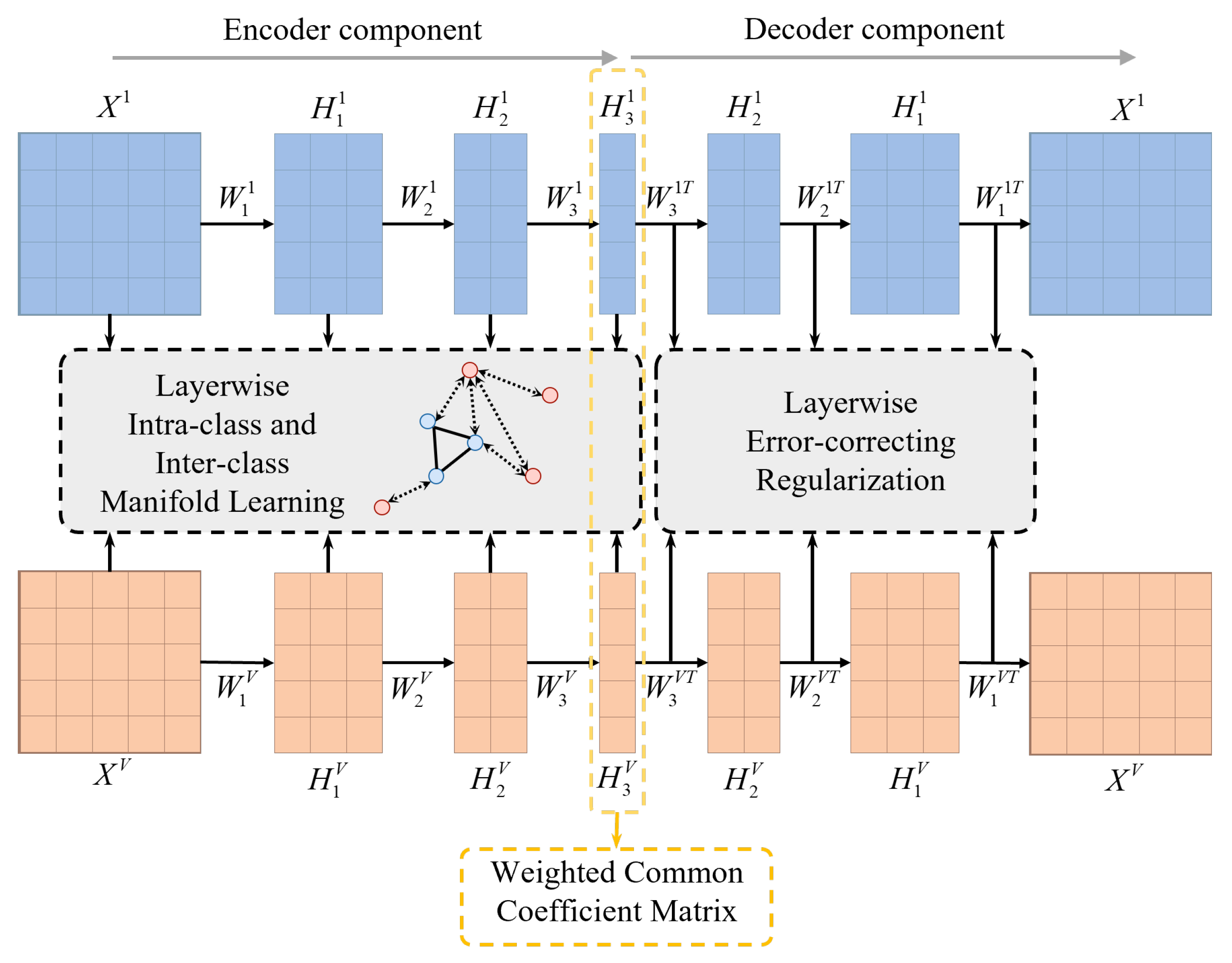
As shown in Figure 1, the proposed framework consists of four key components, each designed to enhance the effectiveness of MVC through deep NMF, manifold learning, error correction, and self-weighted consensus modeling.
First, an autoencoder-inspired deep NMF model is introduced to decompose each view’s data into a coefficient matrix and a set of basis matrices. This approach enables the reconstruction of the original data matrix while simultaneously mapping it into a lower-dimensional space under appropriate constraints. By leveraging deep factorization, the model captures complex hierarchical structures, extracts more interpretable components, and strengthens the correlation between the learned representations and the original data. This step ensures that the essential characteristics of each data view are preserved and effectively utilized in downstream clustering tasks.
Second, a layerwise intra-class and inter-class manifold learning mechanism is incorporated to maintain the inherent geometric structure of the data. This mechanism is essential for ensuring that similar samples are grouped closely together while dissimilar ones are assigned to separate clusters. By integrating manifold learning at each decomposition layer, the framework prevents the loss of local structural relationships and enhances the discriminative power of the learned features. This structure-preserving property is particularly beneficial in high-dimensional and complex data environments where conventional clustering approaches often struggle to maintain meaningful feature separations.
Third, layerwise error constraints are applied to reduce reconstruction errors at each stage of matrix decomposition. Rather than relying solely on a global reconstruction loss, constraints are enforced at each layer to refine intermediate factorization results and progressively correct deviations. This localized optimization approach prevents error accumulation, leading to more stable and accurate low-dimensional representations. As the decomposition process progresses, this mechanism mitigates the risk of feature divergence, ensuring that the final representations remain closely aligned with the actual intrinsic structure of the data.
Finally, a self-weighted consensus matrix is introduced, allowing for adaptive weight adjustments across different views. The weight assignments are iteratively updated to enable all views to contribute meaningfully to the final clustering indicator matrix. This consensus mechanism ensures that views with higher-quality representations exert greater influence while mitigating the impact of less informative or noisy views. The integration of self-weighted learning enhances the robustness of the clustering process, leading to more reliable and interpretable results.
By systematically incorporating these four components, the proposed framework effectively balances feature extraction, structure preservation, error correction, and adaptive weighting. These aspects make it well suited for addressing complex MVC tasks.

3.2. Deep Autoencoder-Inspired NMF for MVC

Notably, in the MVC frameworks, the data inherently comes from diverse sources or modalities (views), each capturing unique yet complementary aspects of the shared underlying structure. Through systematic dimensionality reduction, the encoder architecture maps high-dimensional input data from individual views into lower-dimensional latent spaces, a process that not only preserves discriminative features but also eliminates redundant information. This mechanism enables effective feature extraction while maintaining clustering-critical data characteristics.
Building upon this foundation, the hierarchical learning paradigm facilitates the progressive abstraction of features, thereby capturing both elementary patterns and sophisticated high-level structures. As demonstrated by Liu et al. [22], the consensus matrix approach exhibits marked advantages over fixed coefficient matrices, primarily attributed to its inherent capacity to model cross-view structural dependencies. Furthermore, view-specific weight allocation—as rigorously investigated in [21]—emerges as a critical component for optimizing MVC performance, since differentiated contribution weighting better accommodates view heterogeneity.
For multiview data matrices X = { X 1 , X 2 , , X v } , based on these ideas, a unified framework for MVC can be expressed as Equation (5):
min W 1 v , , W m v , H m v v = 1 V X v W 1 v W 2 v W m v H m v F 2 + H m v W m v T W 2 v T W 1 v T X v F 2 + ( α v ) γ H v H * F 2 , s . t . H m v 0 , W i v 0 , i = 1 , 2 , , m .
where α v is the weight of the vth view updated with iteration and γ v is the hyperparameter to control the weights distribution.

3.3. Layerwise Error-Correcting Regularization

Existing DNMF methods are merely an extension of the standard single-layer matrix decomposition following Trigeorgis’s work. During the matrix decomposition process, local errors at each layer are not independently accounted for; instead, they are constrained only by a global reconstruction error loss function. As a result, the model lacks the ability to optimize each decomposition layer individually. This limitation can lead to the accumulation of significant errors in critical layers, ultimately affecting the overall decomposition quality and clustering performance. As the number of matrix decomposition layers increases, these errors continue to build up, potentially causing the final low-dimensional features to deviate from the actual intrinsic structure of the data. This divergence can reduce the model’s reliability and practical applicability.
To overcome the above issues, a layerwise error-correcting regularization term is proposed to measure and constrain the decomposition error of each layer on the basis of the original loss function, as in Equation (6)
min W i v , H i v i = 1 m H i 1 v W i v H i v F 2 , s . t . H i v 0 , W i v 0 , i = 1 , 2 , , m ,
where H i 1 v denotes the coefficient matrix obtained by factorization on the last layer, W i v and H i v indicate the basic matrix and coefficient matrix obtained by factorization on this layer, and  H 0 = X for format standardization.

3.4. Layerwise Graph Regularization for Intra-Class Similarity and Inter-Class Difference

Conventional graph regularization mechanisms in NMF predominantly focus on intra-class attraction forces, where geometrically similar samples are compelled to maintain proximity within the latent representation space. While this approach proves effective for homogeneous data clusters, it introduces unintended effects when handling dissimilar sample pairs, potentially causing inappropriate approximation of heterogeneous instances. This inherent limitation becomes particularly acute in MVC scenarios, where view-specific similarity metrics and contribution weights often exhibit substantial divergence across modalities.
Building upon the contrastive learning principle that explicitly differentiates between positive (similar) and negative (dissimilar) pairs, a dissimilarity repulsion term is introduced into the proposed NMF framework. Notably, this term systematically enlarges the distances between dissimilar samples while simultaneously enhancing inter-class discriminative learning. As a direct consequence of integrating this repulsive mechanism, the model improves the preservation of intrinsic class distinctions. Furthermore, to maintain geometric consistency across multiview representations, graph regularization constraints are uniformly imposed throughout all decomposition layers, thus ensuring manifold structure alignment between original data spaces and learned latent embeddings.
The KNN algorithm is used to identify the nearest neighbors and construct the intra-class attractive matrix S i a ( v ) term and inter-class repulsive matrix S i r ( v ) for view v, calculated as Equations (7) and (8):
S i ( j k ) a ( v ) = exp h i ( j ) v h i ( k ) v 2 2 ( t v ) 2 , if h i ( j ) v K ( h i ( k ) v ) or h i ( k ) v K ( h i ( j ) v ) , 0 , otherwise ,
S i ( j k ) r ( v ) = exp h i ( j ) v h i ( k ) v 2 , if h i ( j ) v K ( h i ( k ) v ) or h i ( k ) v K ( h i ( j ) v ) , 0 , otherwise ,
where h i ( j ) v denotes data point h ( j ) v in the i-th layer, K ( h i ( j ) v ) indicates the k-nearest neighborhood of data point h i ( j ) v , and  t v is a constant.
The attractive manifold learning term and repulsive manifold learning term can be formulated using the Laplacian matrix as L i a ( v ) = D i a ( v ) S i a ( v ) and L i r ( v ) = D i r ( v ) S i r ( v ) , where D i a ( v ) and D i r ( v ) is the diagonal matrix of S i a ( v ) and S i r ( v ) , calculated as D i ( j j ) a ( v ) = k = 1 n S i ( j k ) a ( v ) and D i ( j j ) r ( v ) = k = 1 n S i ( j k ) r ( v ) . The graph regularization term is defined as Equation (9):
min W i v , H i v v = 1 V i = 1 m ( T r ( H i v L i a ( v ) H i v T ) T r ( H i v L i r ( v ) H i v T ) ) .

3.5. Objective Function

By integrating three distinct regularization terms in Equations (5), (6) and (9), the overall objective function of MVDALE-NMF can be reformed as Equation (10):
min W i v , H i v O = v = 1 V ( X v W 1 v W 2 v W m v H m v F 2 + H m v W m v T W 2 v T W 1 v T X v F 2 + δ i = 1 m H i 1 v W i v H i v F 2 + λ v = 1 V i = 1 m ( T r ( H i v L i a ( v ) H i v T ) T r ( H i v L i r ( v ) H i v T ) ) + ( α v ) γ H m v H * F 2 ) , s . t . H i v , W i v , H * 0 , i = 1 , 2 , , m , v = 1 V ( α v ) γ = 1 ,
where δ , λ , γ are three hyperparameters controlling the weight of layerwise error-correcting, intra-class and inner-class graph regularization, and common matrix components, respectively. A systematic examination of the parameter analysis is provided in Section 5.6.

4. Optimization

This section begins by introducing the pre-training strategy employed in the proposed framework. Subsequently, the update rules for each component are systematically derived. The theoretical proof of convergence for these update rules is then presented. Finally, the time complexity of the framework is analyzed to assess its computational efficiency.

4.1. Pre-Training

By adopting a layer-wise pre-training strategy [42,43], the current model achieves accelerated factor reconstruction. Each hierarchical layer is independently initialized to generate preliminary approximations of the matrices W i and H i . This strategy has been empirically shown to lead to a substantial reduction in the model’s training time. The pre-training process is carried out by factorizing the coefficient matrix of the last layer H i 1 W i H i with minimizing H i 1 W i H i F 2 + H i W i T H i 1 F 2 . This iterative process continues until all decomposition layers complete their pre-training phase. Subsequently, an alternating minimization algorithm is applied to systematically refine the parameters of each layer.

4.2. Updating Rules

The objective function Equation (10) can be rewritten in the form of the trace of the matrix as follows:
min W i v , H i v O = v = 1 V ( T r ( H 0 v T H 0 v + H m T H m 4 H 0 v T Ψ i 1 W i v Φ i + 1 H m v + H m T Φ i + 1 T W i T Ψ i 1 T Ψ i 1 W i Φ i + 1 H m + H 0 T Ψ i 1 W i Φ i + 1 Φ i + 1 T W i T Ψ i 1 T H 0 ) + δ i = 1 m T r ( H i 1 v T H i 1 v 2 H i 1 v T W i v H i v + H i v T W i v T W i v H i v ) + λ i = 1 m T r ( H i v T L i a ( v ) H i v H i v T L i r ( v ) H i v ) + ( α v ) γ T r ( H m v T H m v 2 H m v T H * + H * T H * ) ) , s . t . H i v , W i v , H * 0 , i = 1 , 2 , , m , v = 1 V ( α v ) γ = 1 ,
where Ψ i 1 = W 1 W 2 W i 1 and Φ i + 1 = W i + 1 W i + 2 W m . When i = 1 , Ψ 0 = I is set in this paper. Similarly, when i = m , Φ m = I is set in this paper.

4.2.1. Updating Rule of the Basis Matrix W i v ( 1 i m )

Given the fixed parameters H i v , H * , and ( α v ) γ , it necessarily follows that the optimization problem for W i v in Equation (11) reduces to:
min W i v O ( W i v ) = T r 4 H 0 v T Ψ i 1 v W i v Φ i + 1 v H m v + H m v T Φ i + 1 v T W i v T Ψ i 1 v T Ψ i 1 v W i v Φ i + 1 v H m v + H 0 v T Ψ i 1 v W i v Φ i + 1 v Φ i + 1 v T W i v T Ψ i 1 v T H 0 v + δ T r 2 H i 1 v H i v T W i v T + W i v H i v H i v T W i v T , s . t . W i v 0 , i = 1 , 2 , , m .
To resolve this constrained formulation, a Lagrangian multiplier θ W i v is defined to impose non-negative constraints on W i v , which directly leads to:
L ( W i v , θ W i v ) = O ( W i v ) T r ( θ W i v W i v T ) .
Through differentiation, the partial derivatives are obtained as follows:
L ( W i v , θ W i v ) W i v = 4 Ψ i 1 v T H 0 v H m v T Φ i + 1 v T + 2 Ψ i 1 v T Ψ i 1 v W i v Φ i + 1 v H m v H m v T Φ i + 1 v T + 2 Ψ i 1 v T H 0 v H 0 v T Ψ i 1 v W i v Φ i + 1 v Φ i + 1 v T 2 δ H i 1 v H i v T + 2 δ W i v H i v H i v T θ W i .
By enforcing the Karush–Kuhn–Tucker (KKT) conditions θ W i v W i v = 0 , the ultimate update rule for W i v emerges:
W i v W i v 2 Ψ i 1 v T H 0 v H m v T Φ i + 1 v T + δ H i 1 v H i v T Ψ i 1 v T Ψ i 1 v W i v Φ i + 1 v H m v H m v T Φ i + 1 v T + Ψ i 1 v T H 0 v H 0 v T Ψ i 1 v W i v Φ i + 1 v Φ i + 1 v T + δ W i v H i v H i v T + ϵ .
where ∘ denotes the elementwise multiplication, and  ϵ is a small constant introduced to prevent division by zero.

4.2.2. Updating Rule of the Coefficient Matrix H i v ( 1 i m )

(1) 1 i < m .
Under the condition of fixed W i v , H * , and ( α v ) γ , a parallel derivation process reveals the H i v -oriented objective function:
min H i v O ( H i v ) = T r 2 H i 1 v H i v T W i v + W i v H i v H i v T W i v T + δ T r H i v H i v T 2 H i v H i + 1 v T W i + 1 v T + λ T r H i v L i a ( v ) H i v T H i v L i r ( v ) H i v T , s . t . H i v 0 , i = 1 , 2 , , m ,
Consistent with the methodology, the Lagrangian multiplier θ H i v is incorporated to impose non-negative constraints on H i v , yielding:
L ( H i v , θ H i v ) = O ( H i v ) T r ( θ H i v H i v T ) .
Systematic differentiation produces:
L ( H i v , θ H i v ) H i v = 2 W i v H i 1 v + 2 H i v T W i v T W i v T + 2 δ H i v 2 δ W i + 1 v H i + 1 v + 2 λ L i a ( v ) 2 λ L i r ( v ) θ H i .
Application of KKT conditions θ H i v H i v = 0 , gives rise to:
H i v H i v W i v T H i 1 v + δ W i + 1 v H i + 1 v + λ H i v S i a ( v ) + λ H i v D i r ( v ) W i v T W i v H i v + δ H i v + λ H i v D i a ( v ) + λ H i v S i r ( v ) + ϵ .
(2) i = m .
With frozen variables W i v , H * , and ( α v ) γ are fixed, an isomorphic computational pathway derives the H m v update framework:
min H m v O ( H m v ) = T r H m v T H m v 4 H 0 v T Ψ m v H m v + H m v T Ψ m v T Ψ m v H m v + δ T r 2 H m 1 v H m v T W m v T + W m v H m v H m v T W m v T + λ T r H m v L m a ( v ) H m v T H m v L m r ( v ) H m v T + ( α v ) γ T r H m v T H m v 2 H m v ( H * ) v T , s . t . H m v 0 .
Following the established protocol, θ H m v is introduced, generating:
L ( H m v , θ H m v ) = O ( H m v ) T r ( θ H m v H m v T ) .
Derivative computation yields:
L ( H m v , θ H m v ) H m v = 2 H m v 4 Ψ m v T H 0 v + 2 Ψ m v T Ψ m v H m v 2 δ H m 1 v + 2 δ W m v T W m v H m v + 2 λ L m a ( v ) 2 λ L m r ( v ) + 2 ( α v ) γ H m v 2 ( α v ) γ H * .
Strict adherence to KKT conditions θ H m v H m v = 0 establishes:
H m v H m v 2 Ψ m v T H 0 v + δ W m v T H m 1 v + ( α v ) γ H * + λ v H m v S m a ( v ) + λ v H m v D m r ( v ) Ψ m v T Ψ m v H m v + δ W m v T W m v H m v + ( 1 + ( α v ) γ ) H m v + λ v H m v D m a ( v ) + λ v H m v S m r ( v ) + ϵ .

4.2.3. Updating Rule of the Common Matrix H *

Given the invariance of W i v , H i v , and ( α v ) γ , a direct corollary emerges for the H * parameter optimization:
min H * O ( H * ) = v = 1 V ( α v ) γ T r ( H m v T H m v 2 H m v T H * + H * T H * ) , s . t . H * 0 .
The partial derivative with respect to H * is necessarily derived as follows:
O ( H * ) H * = 2 v = 1 V ( α v ) γ H m v + 2 v = 1 V ( α v ) γ H * = 0 .
The updating rule for H * is as follows:
H * = v = 1 V ( α v ) γ H m ( v ) v = 1 V ( α v ) γ .

4.2.4. Updating Rule of the Weight of View ( α v )

Assuming fixed values for W i v , H i v , and H * , the immediate consequence is the simplified optimization target for ( α v ) :
min α v O ( α v ) = v = 1 V ( α v ) γ T r ( H m v T H m v 2 H m v T H * + H * T H * ) , s . t . v = 1 V ( α v ) γ = 1 .
Similar to [44], to impose non-negativity constraints, the Lagrangian multiplier θ α v is incorporated, thereby formulating:
L ( α v , θ α v ) = v = 1 V ( α v ) γ C v θ α v v = 1 V α v 1 ,
where C v denotes T r ( H m v T H m v 2 H m v T H * + H * T H * ) . Setting the derivatives of O ( H * ) with respect to H * to zero yields:
α ( v ) = θ α v γ C v 1 γ 1 .
Substitute the resultant α v into the constraint v = 1 V ( α v ) γ = 1 yields:
α ( v ) = γ C v 1 1 γ v = 1 V γ C v 1 1 γ .
Through the aforementioned four steps, W i v , H i v , H * , and ( α v ) γ are successively updated in an alternating manner, and this procedure is iterated until the objective function stabilizes. The proposed algorithm is outlined in Algorithm 1.
Algorithm 1 The algorithm of MVDALE-NMF
  1:
Input: Multiview data { X v } v = 1 V , number of layers m, size of each layer l i , regularization parameters δ , λ , γ .
  2:
Output: Clustering indicator matrix H * .
  3:
[Initialization phase]
  4:
for each view v do
  5:
      Initialize W i > 0 , H i > 0 , H * > 0
  6:
      for view v = 1 to v do
  7:
          for layer i = 1 to m do
  8:
             Construct intra-class graph weight matrix S i a ( v )
  9:
             Construct inter-class graph weight matrix S i r ( v )
10:
        end for
11:
    end for
12:
end for
13:
[Pre-training phase]
14:
for each view v = 1 to n do
15:
    for each layer i = 1 to m do
16:
        Update W i v , H i v using Autoencoder-inspired NMF
17:
    end for
18:
end for
19:
[Fine-tuning phase]
20:
while not reach stopping criterion do
21:
    for each view v = 1 to n do
22:
        for each layer i = 1 to m do
23:
              Update W i v based on Equation (15)
24:
              if  1 i < m  then
25:
                 Update H i v based on Equation (19)
26:
              end if
27:
              if  i = m  then
28:
                 Update H m v based on Equation (23)
29:
              end if
30:
          end for
31:
    end for
32:
    Update H * based on Equation (26)
33:
    Update α v based on Equation (30)
34:
end while
35:
Apply clustering algorithm to H * to obtain the clustering results

4.3. Convergence of the Algorithm

The convergence of the proposed Algorithm 1 is theoretically proved in this subsection. Given the non-negativity constraint of the objective function, the lower bound of the iterative updates is naturally zero. Therefore, only the monotonicity of the updating rules needs to be proved. Moreover, the optimal solution for H * and α v has been derived. Therefore, only the convergence of the updating rules for W i v , H i v , and H m v needs to be proved.
Theorem 1. 
The objective function Equation (10) is nonincreasing under the updating rules Equations (15), (19) and (23).
To prove the theorem, an auxiliary function, as defined in [17], is introduced. The definition is provided below.
Definition 1. 
For any given h and h , if the conditions
G ( h , h ) F ( h ) , G ( h , h ) = F ( h )
are satisfied, G ( h , h ) is an auxiliary function for F ( h )
Using the auxiliary function, monotonicity can be established based on the following lemma [17].
Lemma 1. 
If G is an auxiliary function, then F is nonincreasing under the update
h t + 1 = arg min h G ( h , h t ) ,
where t denotes the t-th iteration.
Proof. 
F ( h t + 1 ) G ( h t + 1 , h t ) G ( h t , h t ) = F ( h t )
For variant W i v , according to Lemma 1, an appropriate auxiliary function needs to be constructed to prove the convergence of the objective function Equation (10) under the updating rule Equation (15). Fixing parameters H i v , H * , and ( α v ) γ , the optimization problem for W i v reduces to:
min W i v O ( W i v ) = T r 4 H 0 v T Ψ i 1 v W i v Φ i 1 v H m v + H m v T Φ i + 1 v T W i v T Ψ i 1 v T Ψ i 1 v W i v Φ i + 1 v H m v + H 0 v T Ψ i 1 v W i v Φ i + 1 v Φ i + 1 v T W i v T Ψ i 1 v T H 0 v + δ T r 2 H i 1 v H i v T W i v T + W i v H i v H i v T W i v T , s . t . W i v 0 , i = 1 , 2 , , m .
The first and second derivatives of Equation (33) are as follows:
O ( W i v ) = 4 Ψ i 1 v T H 0 v H m v T Φ i + 1 v T + 2 Φ i + 1 v T H m v T H m v Φ i + 1 v Ψ i 1 v Ψ i 1 v T W i v + 2 Φ i + 1 v T Φ i + 1 v Ψ i 1 v H 0 v T H 0 v Ψ i 1 v T W i v 2 δ H i 1 v H i v T + 2 δ H i v T H i v W i v .
O ( W i v ) = 2 Φ i + 1 v T H m v T H m v Φ i + 1 v Ψ i 1 v Ψ i 1 v T + 2 Φ i + 1 v T Φ i + 1 v Ψ i 1 v H 0 v T H 0 v Ψ i 1 v T + 2 δ H i v T H i v .
The second-order Taylor series of Equation (33) is presented as follows:
O ( W i v ) = O ( W i v t ) + q , r O ( W i v t ) q r W i v W i v t q r + q , r O ( W i v t ) q r 2 W i v W i v t q r 2 .
The auxiliary function for O ( W i v ) can be constructed.
Lemma 2. 
Function G ( W i v , W i v t ) is an auxiliary function for O ( W i v ) , where
G ( W i v , W i v t ) = O ( W i v t ) + q , r O ( W i v t ) q r W i v W i v t q r + q , r Φ i + 1 v T H m v T H m v Φ i + 1 v Ψ i 1 v Ψ i 1 v T + Φ i + 1 v T Φ i + 1 v Ψ i 1 v H 0 v T H 0 v Ψ i 1 v T + δ H i v T H i v W i v q r W i q r v t W i v W i v t q r 2 .
Proof. 
To prove that G ( W i v , W i v t ) is the auxiliary function of O ( W i v ) , it only needs to be shown that G ( W i v , W i v ) = O ( W i v ) and G ( W i v , W i v t ) O ( W i v ) holds. According to Definition 1, G ( W i v , W i v ) = O ( W i v ) is clear. Proving G ( W i v , W i v t ) O ( W i v ) is equivalent to proving:
Φ i + 1 v T H m v T H m v Φ i + 1 v Ψ i 1 v Ψ i 1 v T + Φ i + 1 v T Φ i + 1 v Ψ i 1 v H 0 v T H 0 v Ψ i 1 v T + δ H i v T H i v W i v q r W i q r v t O ( W i v t ) q r 2 .
The following formula holds:
Φ i + 1 v T H m v T H m v Φ i + 1 v Ψ i 1 v Ψ i 1 v T + Φ i + 1 v T Φ i + 1 v Ψ i 1 v H 0 v T H 0 v Ψ i 1 v T + δ H i v T H i v W i v q r = s = 1 f Φ i + 1 v T H m v T H m v Φ i + 1 v Ψ i 1 v Ψ i 1 v T + Φ i + 1 v T Φ i + 1 v Ψ i 1 v H 0 v T H 0 v Ψ i 1 v T + δ H i v T H i v q s ( W i v ) s r Φ i + 1 v T H m v T H m v Φ i + 1 v Ψ i 1 v Ψ i 1 v T + Φ i + 1 v T Φ i + 1 v Ψ i 1 v H 0 v T H 0 v Ψ i 1 v T + δ H i v T H i v q q ( W i v ) q r .
Therefore, G ( W i v , W i v t ) O ( W i v ) has been proved. And G ( W i v , W i v t ) is an auxiliary function of O ( W i v ) . □
The convergence of Theorem 1 can now be demonstrated.
Proof of Theorem 1. 
Since G ( W i v , W i v t ) is a convex quadratic, replacing G ( h , h t ) in Lemma 1 by G ( W i v , W i v t ) , its optimal solution is obtained as follows:
W i v = ( W i v ) q r O ( ( W i v ) q r ) 2 Φ i + 1 v T H m v T H m v Φ i + 1 v Ψ i 1 v Ψ i 1 v T W i v + Φ i + 1 v T Φ i + 1 v Ψ i 1 v H 0 v T H 0 v Ψ i 1 v T W i v + δ H i v T H i v W i v q r = ( W i v ) q r 2 Ψ i 1 v T H 0 v H m v T Φ i + 1 v T + δ H i 1 v H i v T Ψ i 1 v T Ψ i 1 v W i v Φ i + 1 v H m v H m v T Φ i + 1 v T + Ψ i 1 v T H 0 v H 0 v T Ψ i 1 v W i v Φ i + 1 v Φ i + 1 v T + δ W i v H i v H i v T q r .
This is in full agreement with Equation (15). Since G ( W i v , W i v t ) is an auxiliary function of O ( W i v ) , that is, the part of the objective function Equation (10) which is related to ( W i v ) , Equation (10) is nonincreasing under updating rule Equation (15) according to Lemma 1. Following identical procedures, the auxiliary functions of H i v and H m v can be constructed, and Equation (10) can be proven to be nonincreasing under the updating rule given by Equation (19) and Equation (23). Therefore, Theorem 1 is proved. □

4.4. Complexity Analysis

Algorithm 1 comprises three main stages: an initialization phase, a pre-training phase, and a fine-tuning phase. Accordingly, the time complexity of each phase is analyzed separately. For simplicity, let l represent the maximum layer size across all layers, d the maximum feature dimension among all views, n the number of samples, V the number of views, and m the number of layers.
In the initialization phase, let k denote the neighborhood size to construct a kNN graph; the complexity of graph Laplacian on all views is O ( m V n 2 k ) . The complexity of the pre-training phase is O ( T p m V ( n d l + n l 2 + d l 2 ) ) , where T p denotes the iteration times of the pre-training phase. During the fine-tuning phase, for each iteration of each view, the complexity of updating W i v in Equation (15) is 3 n d l + 11 n 2 l + 2 d l 2 + 3 l 3 , the complexity of updating H i v in Equation (19) is 7 n l 2 , and the complexity of updating H m v in Equation (23) is n d l + d l 2 + 7 n l 2 + l 3 . Let T f denote the iteration times of the fine-tuning phase; the complexity of the fine-tuning phase is T f V ( ( 3 m + 1 ) n d l + 18 m n l 2 + ( 2 m + 1 ) d l 2 + ( 3 m + 1 ) l 3 ) . Therefore, with V views, the overall complexity of the proposed MVDALE-NMF algorithm is O ( m V n 2 k + ( T p + T f ) m V ( n d l + n l 2 + d l 2 ) ) . Due to m , l being negligible compared to n , d , the MVDALE-NMF algorithm has a quadratic complexity.

5. Experiments

5.1. Datasets

A number of real-world multiview datasets are utilized in the experiments to evaluate the performance of the proposed model. A concise overview of the datasets is given below, and some important statistics are summarized in Table 1.
  • ALOI-100 (https://github.com/JethroJames/Awesome-Multi-View-Learning-Datasets (accessed on 3 April 2024)): The Amsterdam Library of Images (ALOI) [45] comprises 110,250 samples sourced from 1000 small objects. Each object has an average of 100 samples. The ALOI-100 dataset is created by extracting the initial 100 object types from ALOI, comprising 10,800 color images, with each sample described by four views: 77 color similarity features, 13 Haralick features, 64 HSV features, and 125 RGB features.
  • Handwritten (https://archive.ics.uci.edu/ml/datasets/Multiple+Features (accessed on 3 April 2024)): The Handwritten dataset is composed of 2000 digit images that have been manually inscribed, with 200 samples for each digit ranging from “0” to “9”. Each image is characterized by six distinct feature sets, including 216 profile correlations, 76 Fourier coefficients of the character shapes, 64 Karhunen–Loève coefficients, 6 morphological features, 240 pixel averages in 2 × 3 windows, and 47 Zernike moments.
  • Leaves (https://archive.ics.uci.edu/dataset/241/one+hundred+plant+species+leaves+data+set (accessed on 3 April 2024)): The Leaves dataset consists of 1600 samples, with 16 leaf samples from each of 100 plant species. Three views are extracted to characterize the samples, i.e., 64 shape features, 64 fine-scale margin histogram features, and 64 texture histogram features.
  • UCI (https://github.com/ChuanbinZhang/Multi-view-datasets (accessed on 3 April 2024)): Following [12], this dataset is similar to the MFEAT dataset; however, each sample is described by three features: 240 pixel averages in 2 × 3 windows, 76 Fourier coefficients of the character shapes, and 6 morphological features.
  • WebKB (http://www.cs.cmu.edu/~webkb/ (accessed on 3 April 2024)): The WebKB dataset consists of 1051 webpage documents sourced from the computer science departments of several universities, categorized into two classes. Each document has two types of features: 3000 dimensions representing the text on the web pages and 1840 dimensions representing the anchor text on the hyperlinks pointing to the page.

5.2. Compared Algorithms

To better highlight the differences between the proposed method and the comparison algorithms, Table 2 summarizes the key distinctions among them.
Additionally, the time complexity of the baseline models is compared in Table 3. For the 2CMV method [46], r represents the new rank value. The computational efficiency of all NMF-based techniques generally follows quadratic time complexity. Notably, NMF [17], DMF [24], and DANMF [34] are single-view approaches; when extended to multiview tasks, their time complexity increases by a factor of v. Among these methods, MVDALE-NMF stands out by significantly improving clustering performance across the evaluation metrics while maintaining comparable computational efficiency to other NMF-based frameworks.

5.2.1. Shallow Matrix Factorization Methods

  • NMF [17]: Standard NMF reduces the dimensionality of the original matrix by finding two non-negative matrices, generating a data feature matrix with reduced dimensions.
  • MultiNMF [22]: MultiNMF is a multiview NMF method with local graph regularization to preserve the geometric structure of each view. It employs a joint matrix factorization process that aims to achieve a common consensus by constraining the coefficient matrices of different views.
  • 2CMV [46]: It uses Coupled Matrix Factorization [47] and NMF to simultaneously learn the consensus and complementary components from multiview data. It proposes an optimal manifold to capture the most consistent representation embedded in high-dimensional multiview data.
  • DA2NMF [37]: It employs an autoencoder-inspired NMF model to learn linear low-dimensional features and introduces adaptive graph learning to capture nonlinear data structures. In addition, a dual auto-weighted strategy is developed to compute weights for different views.

5.2.2. Deep Matrix Factorization Methods

  • DMF [24]: A single view model stacking multiple layers of Semi-NMF to reveal hierarchical, low-dimensional attributes of data.
  • DMVC [25]: It uses deep matrix factorization techniques to extract relevant features from multiple views of data. Moreover, it introduces a weight balance strategy that leverages the complementary information in different views.
  • DANMF [34]: Designed for community detection, DANMF is a hierarchical structure that combines the encoder-decoder architecture of deep autoencoders with deep NMF. The encoder component progressively reduces the dimensionality of the input adjacency matrix, while the decoder component reconstructs the original matrix from the latent space.
  • ODD-NMF [41]: This deep NMF method features a diversity constraint to handle complementary information and an orthogonal constraint to guarantee the uniqueness of the clustering. In addition, it preserves the geometric structure within the data by applying optimal manifolds to each layer.
  • MGANMF [36]: It integrates deep autoencoder-like NMF with graph regularization to capture the intrinsic geometric structure of multiview data. Additionally, self-updating weights are employed to balance the contributions of each view.

5.3. Experimental Setup

The optimal clustering results of these methods are reported by searching the related parameters in grids. The parameters and iteration counts essential for the algorithm are sourced from the corresponding paper. Single-view clustering algorithms are executed on each view of the dataset, and the best outcomes are documented as the final experimental results. All experiments are conducted on MATLAB R2022a, using a high-performance computer with an R7-5800H CPU and 16 GB of RAM, without GPU, under a Windows 11 system.
Three widely used clustering evaluation criteria, Accuracy (ACC), Normalized Mutual Information (NMI), and F-score are utilized to generally evaluate the clustering performance of all methods. The higher the values of these matrices, the better the clustering performance.

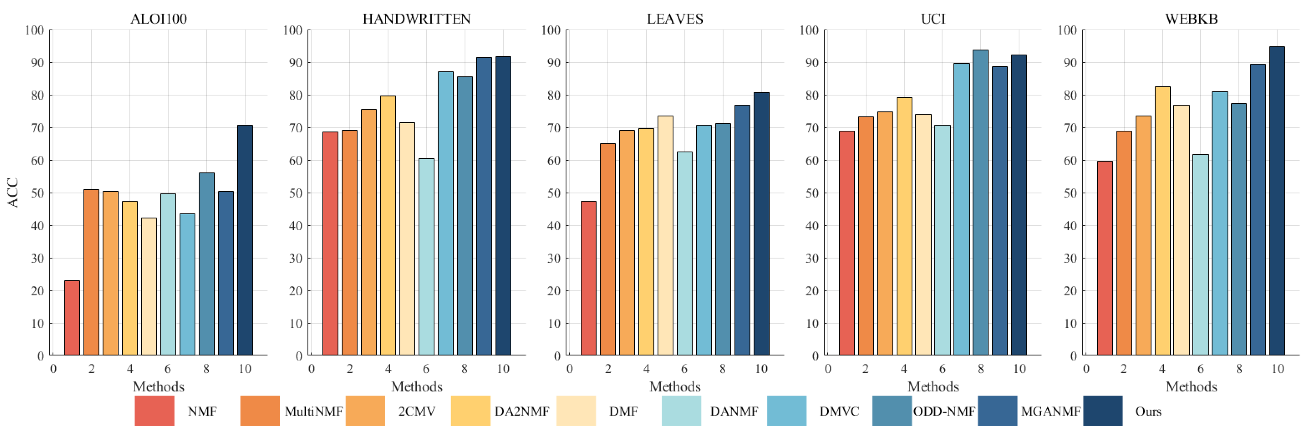
5.4. Clustering Results and Analysis

A substantial number of comparative experiments have been carried out to demonstrate the efficacy of the proposed algorithm. The clustering effect of all algorithms on the ALOI100, Handwritten, Leaves, UCI, and WebKB datasets was evaluated based on three metrics, as illustrated in Table 4, Table 5 and Table 6. In order to achieve a more intuitive comparison, the clustering results have been presented in the form of Figure 2, Figure 3 and Figure 4. The results of our algorithm and the best-performing comparison algorithms are shown in bold, while the second-best results are underlined. The last column presents the average rankings of all compared methods across each evaluation metric.
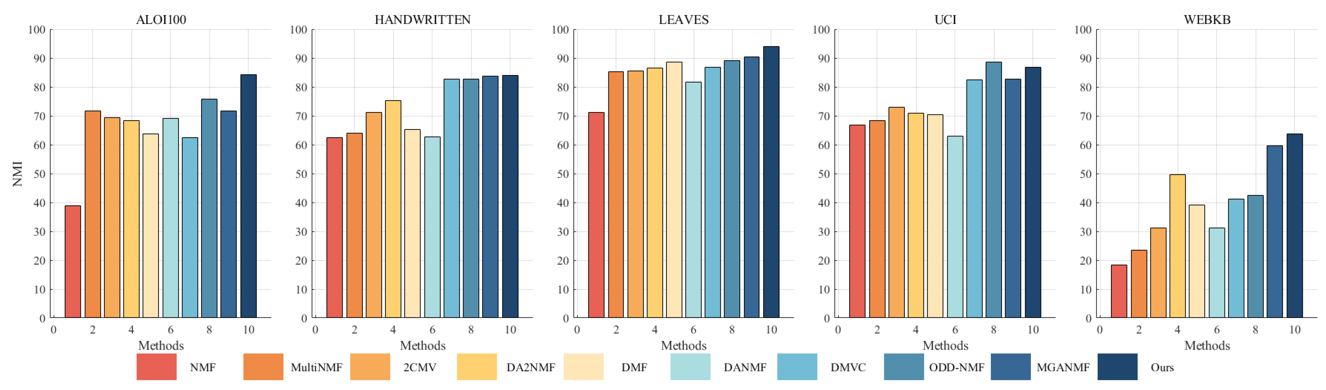
The proposed method consistently demonstrates strong clustering performance, ranking first across most evaluation metrics, with only a few instances where it ranks second or third. On the large-scale dataset aloi100, it significantly outperforms the second-best algorithm, ODD-NMF, with improvements of 26% in ACC, 11% in NMI, and 34% in F-score. This superior performance can be attributed to several key factors: the deep autoencoder-inspired structure that effectively maps data into a latent space, the layer-wise error-correction strategy that refines reconstruction errors at each factorization stage, and intra-class and inter-class graph regularization applied at every layer to preserve the original geometric structure of the data.
The effectiveness of the autoencoder-inspired structures is evident in the comparative analyses. Algorithms such as DANMF and MGANMF, which incorporate encoder components, consistently outperform DMF and DMVC, which do not. The encoder component plays a crucial role in mapping raw data into a lower-dimensional latent space, allowing for the extraction of more meaningful latent features. This process leads to improved clustering performance and higher metric scores.
Another key observation is that models incorporating manifold learning at every layer outperform those that apply graph regularization only at the top layer. Both ODD-NMF and the proposed method, which integrate manifold learning throughout multiple layers, demonstrate superior performance compared to algorithms that restrict graph regularization to a single layer. By applying manifold learning across all layers, these models enhance the ability to maintain the intrinsic structure of the data, resulting in better clustering outcomes.
These findings highlight the advantages of deep structured learning, adaptive reconstruction refinement, and multi-layer regularization, confirming the robustness of the proposed method in handling complex clustering tasks.

5.5. Compared with Other Methods

This subsection compares other machine learning-based MVC methods, including the graph clustering method, Diversity-Induced Bipartite Graph Fusion for Multiview Graph Clustering [48], the subspace clustering method, Nonconvex Low-Rank and Structure-Constrained Multiview Subspace Clustering [49], and the spectral clustering method, Reliable Multiview Graph Learning [50], as shown in Table 7. Our method demonstrates superior performance on most datasets

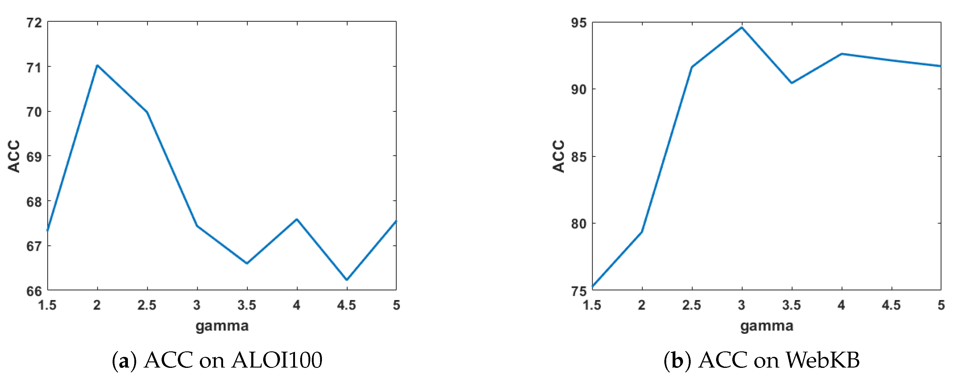
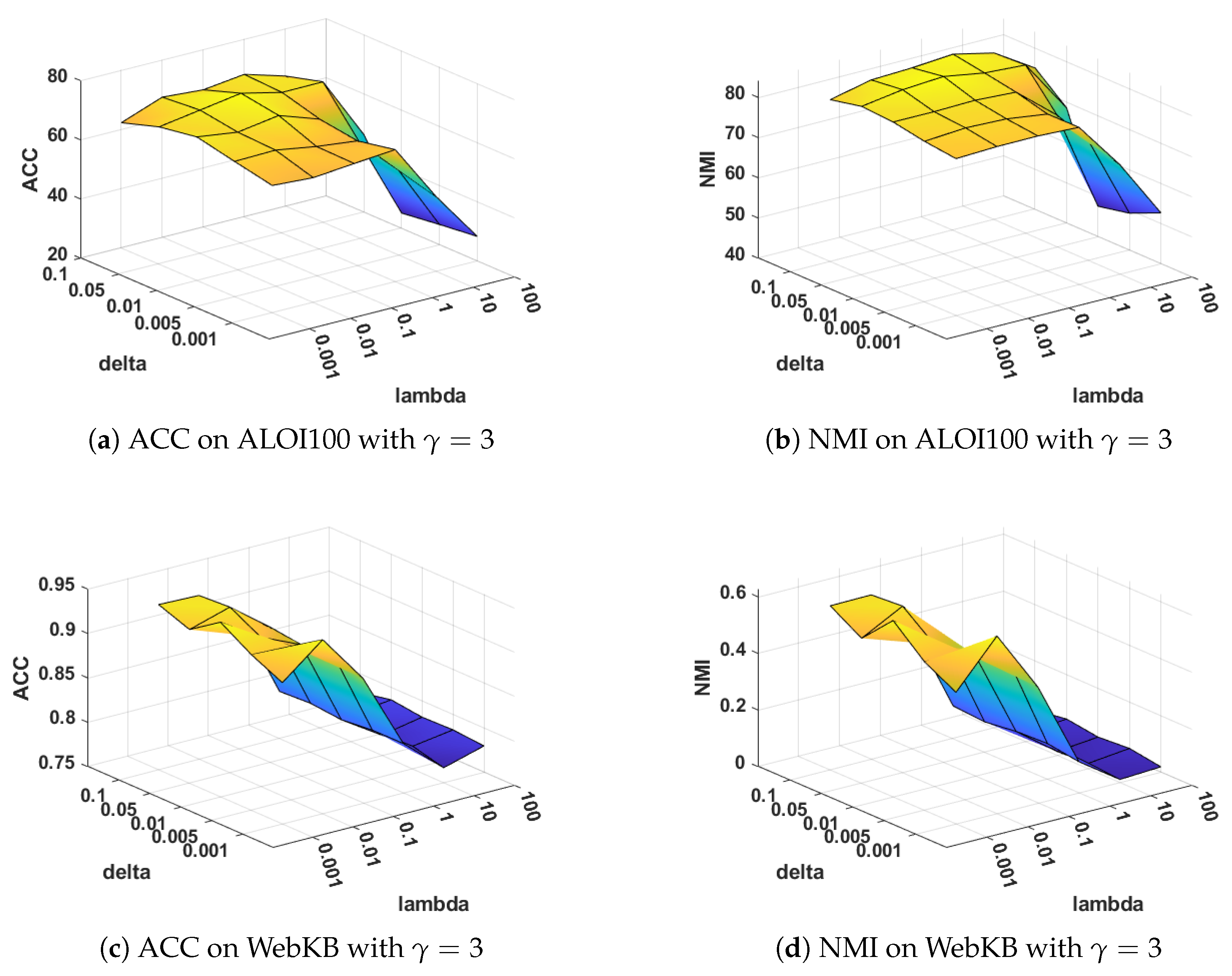
5.6. Parameter Analysis

Sensitivity analysis on γ : The parameter γ balances the weight of different views. When γ = 0, it can be shown that the weights of all views are equal to 1, thereby resulting in a configuration where the weights are equal. Figure 5 demonstrates the clustering ACC and NMI of MVDALE-NMF when γ varies from 1.5 to 5 in steps of 0.5 on the ALOI100 and WebKB dataset.
Sensitivity analysis on λ and δ : The parameters λ and δ are used to balance the layer-wise manifold regularization and layer-wise reconstruction, respectively. Figure 6 and Figure 7 illustrate the clustering performance of MVDALE-NMF in terms of ACC and NMI as λ and δ vary over the ranges [0.001, 0.01, 0.1, 1, 10, 100] and [0.001, 0.005, 0.01, 0.05, 0.1], under two different configurations of γ = 2 and γ = 3 . On the ALOI100 dataset, it is observed that even with a high graph regularization weight ( λ = 100 ), the clustering performance remains competitive, demonstrating the robustness of the layer-wise reconstruction mechanism.

5.7. Ablation Experiment

This subsection evaluates five versions of the proposed framework using the ALOI100 and WebKB datasets: (1) The complete framework (MVDALE-NMF); (2) A version without both attractive and repulsive manifold learning regularizations (− w/o L M ); (3) A version without repulsive manifold learning regularization (− w/o L R ); (4) A version without the error-correcting constraint (− w/o L E ); (5) A version without adaptive weighting (− w/o L α ). As shown in Table 8 and Table 9, setting equal weights for all views leads to a significant drop in clustering performance. This result underscores the importance of adaptive weight allocation across views in MVC. In addition, the attractive and repulsive manifold learning regularizations contribute notably to performance, particularly in image-rich datasets such as ALOI.
Furthermore, the error-correcting constraint has a more substantial impact on the ALOI dataset, likely due to its larger sample size and higher feature dimensionality. These characteristics demand deeper decomposition layers, which, in turn, lead to greater error accumulation, making error correction especially beneficial.
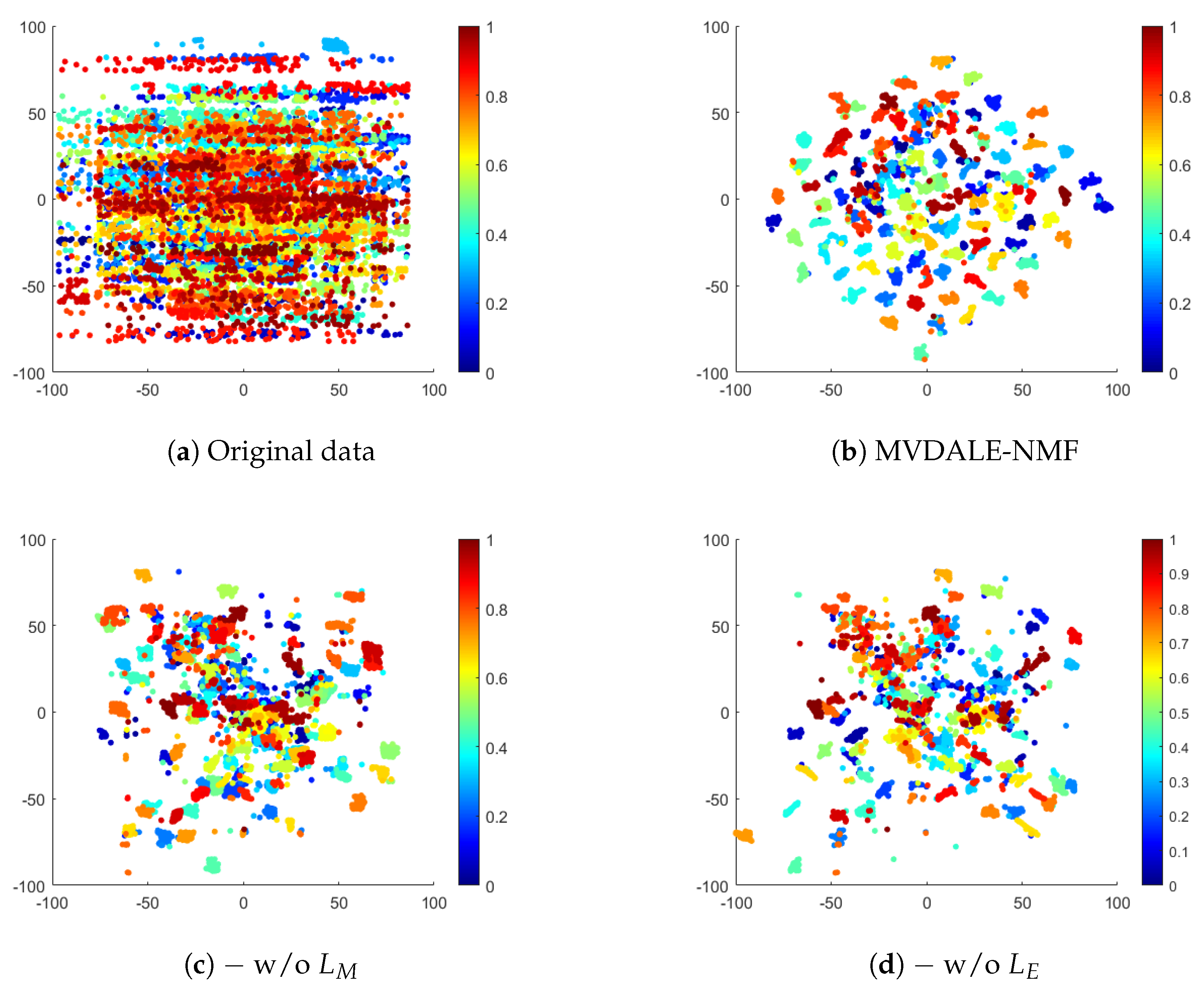
To illustrate the impact of layerwise error correction and manifold learning, the latent representations of the complex ALOI100 dataset are visualized using the t-SNE technique, as shown in Figure 8. Figure 8b demonstrates that the proposed framework effectively clusters and separates samples into distinct groups, indicating a well-learned representation.
The layer-wise error-correcting constraint is designed to align features across different layers, ensuring consistency throughout the learning process. Without this constraint, deep NMF may accumulate reconstruction errors during successive factorizations, resulting in disorganized feature representations. This effect is evident in Figure 8d, where sample points appear more dispersed and the cluster boundaries are less defined, reflecting a lack of structural clarity due to the absence of error correction.
The graph regularization term, on the other hand, preserves the local manifold structure by maintaining sample similarity. Without it, deep NMF is unable to fully leverage the geometric information inherent in the data, limiting its ability to mine collaborative information across views in MVC. This is illustrated in Figure 8c, where samples from the same category are poorly aggregated and significant inter-cluster overlap is observed. The lack of manifold regularization prevents the model from enforcing the structural constraints necessary for effective clustering.

6. Conclusions

This paper addresses the limitations of the shallow matrix factorization models used in MVC tasks, in particular, their inability to capture hierarchical data structures and lack of an efficient mechanism for encoding raw data into latent features. To address these weaknesses, a new MVDALE-NMF is proposed. The model integrates a self-encoding architecture within a deep NMF framework, enforcing non-negativity on all matrices to allow direct mapping of original data into a lower-dimensional, interpretable feature space. This facilitates effective feature extraction and supports the accurate reconstruction of original data.
Further, a layerwise error-correcting regularization is introduced to mitigate error accumulation across deeper layers of matrix decompositions, ensuring that each layer’s output remains closely aligned with the input matrix. The model also incorporates layerwise graph regularization to better preserve hierarchical geometric data structures throughout the layers.
An efficient iterative optimization algorithm based on multiplicative update rules helps improve the model’s performance. Empirical evaluations on five real-world datasets demonstrate that the MVDALE-NMF achieves significant improvements over existing state-of-the-art methods in the field. Future work could focus on addressing the sensitivity of NMF to hyperparameters by developing more robust tuning strategies, as well as improving its performance on imbalanced datasets through better initialization methods or incorporating class priors. Additionally, scalability to large datasets could be enhanced by exploring parallel or distributed NMF algorithms to handle high-dimensional data efficiently.

Author Contributions

Conceptualization, Y.L., Y.W. and H.L.; methodology, Y.L. and Y.W.; software, Y.L.; validation, Y.L., Y.W. and Z.Y.; formal analysis, Y.L., H.L. and Z.Y.; investigation, Y.L. and Y.W.; resources, Y.L., Y.W. and H.L.; data curation, Y.L.; writing—original draft preparation, Y.L.; writing—review and editing, Y.W., H.L. and Z.Y.; visualization, Y.L., Y.W. and H.L.; supervision, Y.W. and H.L.; project administration, H.L. and Z.Y.; funding acquisition, Z.Y. All authors have read and agreed to the published version of the manuscript.

Funding

This project received funding from the European Research Council (ERC) under the European Union’s Horizon 2020 research and innovation programme (Grant Agreement No. 864724).

Data Availability Statement

The data presented in this study are available on request from the first author.

Conflicts of Interest

The authors declare no conflicts of interest.

Notations

TrTrace of a matrix
· F Frobenius norm
Hadamard product
nNumber of samples
VNumber of views
dDimension of samples of v-th view
mNumber of layers
X v Original data matrix of v-th view
W i v Basis matrix of the v-th view in the i-th layer
H i v Coefficient matrix of the v-th view in the i-th layer
H i * Common matrix
l n Number of features in the n-th layer
L i v Graph Laplacian matrix of the v-th view in the i-th layer

References

  1. De Handschutter, P.; Gillis, N.; Siebert, X. A Survey on Deep Matrix Factorizations. Comput. Sci. Rev. 2021, 42, 100423. [Google Scholar] [CrossRef]
  2. Zhou, L.; Du, G.; Lü, K.; Wang, L.; Du, J. A Survey and an Empirical Evaluation of Multi-View Clustering Approaches. ACM Comput. Surv. 2024, 56, 3645108. [Google Scholar] [CrossRef]
  3. Huang, H.; Liang, N.; Yan, W.; Yang, Z.; Lit, Z.; Sun, W. Partially Shared Semi-Supervised Deep Matrix Factorization with Multi-View Data. In Proceedings of the 2020 International Conference on Data Mining Workshops (ICDMW), Sorrento, Italy, 17–20 November 2020; pp. 564–570. [Google Scholar] [CrossRef]
  4. Liang, N.; Yang, Z.; Li, Z.; Sun, W.; Xie, S. Multi-View Clustering by Non-Negative Matrix Factorization with Co-Orthogonal Constraints. Knowl.-Based Syst. 2020, 194, 105582. [Google Scholar] [CrossRef]
  5. Wang, Y.X.; Zhang, Y.J. Nonnegative Matrix Factorization: A Comprehensive Review. IEEE Trans. Knowl. Data Eng. 2012, 25, 1336–1353. [Google Scholar] [CrossRef]
  6. Feng, X.R.; Li, H.C.; Li, J.; Du, Q.; Plaza, A.; Emery, W.J. Hyperspectral Unmixing Using Sparsity-Constrained Deep Nonnegative Matrix Factorization with Total Variation. IEEE Trans. Geosci. Remote Sens. 2018, 56, 6245–6257. [Google Scholar] [CrossRef]
  7. Devarajan, K. A Statistical Framework for Non-Negative Matrix Factorization Based on Generalized Dual Divergence. Neural Netw. 2021, 140, 309–324. [Google Scholar] [CrossRef]
  8. Jie, H.; Ning, Z.; Zhao, Q.; Liu, W.; Hu, J.; Gao, J. Multi-View Based Clustering of 3D LiDAR Point Clouds for Intelligent Vehicles. In Proceedings of the AI 2022: Advances in Artificial Intelligence: 35th Australasian Joint Conference, AI 2022, Perth, WA, Australia, 5–8 December 2022; pp. 57–70. [Google Scholar] [CrossRef]
  9. Sun, X.; He, L.; Jiang, H.; Li, R.; Mao, W.; Zhang, D.; Majeed, Y.; Andriyanov, N.; Soloviev, V.; Fu, L. Morphological Estimation of Primary Branch Length of Individual Apple Trees during the Deciduous Period in Modern Orchard Based on PointNet++. Comput. Electron. Agric. 2024, 220, 108873. [Google Scholar] [CrossRef]
  10. Yu, N.; Wu, M.J.; Liu, J.X.; Zheng, C.H.; Xu, Y. Correntropy-Based Hypergraph Regularized NMF for Clustering and Feature Selection on Multi-Cancer Integrated Data. IEEE Trans. Cybern. 2020, 51, 3952–3963. [Google Scholar] [CrossRef] [PubMed]
  11. Pu, X.; Pan, B.; Che, H. Robust Low-Rank Graph Multi-View Clustering via Cauchy Norm Minimization. Mathematics 2023, 11, 2940. [Google Scholar] [CrossRef]
  12. Xia, R.; Pan, Y.; Du, L.; Yin, J. Robust Multi-View Spectral Clustering via Low-Rank and Sparse Decomposition. AAAI 2014, 28, 2149–2155. [Google Scholar] [CrossRef]
  13. Yang, S.; Zhang, L.; He, X.; Yi, Z. Learning Manifold Structures with Subspace Segmentations. IEEE Trans. Cybern. 2019, 51, 1981–1992. [Google Scholar] [CrossRef] [PubMed]
  14. Deng, X.; Zhang, Y.; Gu, F. Fusion and Enhancement of Consensus Matrix for Multi-View Subspace Clustering. Mathematics 2023, 11, 1509. [Google Scholar] [CrossRef]
  15. Xu, C.; Si, J.; Guan, Z.; Zhao, W.; Wu, Y.; Gao, X. Reliable Conflictive Multi-View Learning. In Proceedings of the AAAI Conference on Artificial Intelligence, Vancouver, BC, Canada, 20–28 February 2024; Volume 38, pp. 16129–16137. [Google Scholar] [CrossRef]
  16. Li, C.; Che, H.; Leung, M.F.; Liu, C.; Yan, Z. Robust Multi-View Non-Negative Matrix Factorization with Adaptive Graph and Diversity Constraints. Inform. Sci. 2023, 634, 587–607. [Google Scholar] [CrossRef]
  17. Lee, D.; Seung, H.S. Algorithms for Non-negative Matrix Factorization. In Advances in Neural Information Processing Systems; Leen, T., Dietterich, T., Tresp, V., Eds.; MIT Press: Cambridge, MA, USA, 2000; Volume 13. [Google Scholar]
  18. Guo, Y.T.; Li, Q.Q.; Liang, C.S. The Rise of Nonnegative Matrix Factorization: Algorithms and Applications. Inform. Sci. 2024, 123, 102379. [Google Scholar] [CrossRef]
  19. Luo, P.; Peng, J.; Guan, Z.; Fan, J. Dual Regularized Multi-View Non-Negative Matrix Factorization for Clustering. Neurocomputing 2018, 294, 1–11. [Google Scholar] [CrossRef]
  20. Zong, L.; Zhang, X.; Liu, X. Multi-View Clustering on Unmapped Data via Constrained Non-Negative Matrix Factorization. Neural Netw. 2018, 108, 155–171. [Google Scholar] [CrossRef]
  21. Cai, H.; Liu, B.; Xiao, Y.; Lin, L. Semi-Supervised Multi-View Clustering Based on Constrained Nonnegative Matrix Factorization. Knowl.-Based Syst. 2019, 182, 104798. [Google Scholar] [CrossRef]
  22. Liu, J.; Wang, C.; Gao, J.; Han, J. Multi-View Clustering via Joint Nonnegative Matrix Factorization. In Proceedings of the 2013 SIAM International Conference on Data Mining, Austin, TX, USA, 2–4 May 2013; pp. 252–260. [Google Scholar] [CrossRef]
  23. Zhang, X.; Gao, H.; Li, G.; Zhao, J.; Huo, J.; Yin, J.; Liu, Y.; Zheng, L. Multi-View Clustering Based on Graph-Regularized Nonnegative Matrix Factorization for Object Recognition. Inform. Sci. 2017, 432, 463–478. [Google Scholar] [CrossRef]
  24. Trigeorgis, G.; Bousmalis, K.; Zafeiriou, S.; Schuller, B.W. A Deep Matrix Factorization Method for Learning Attribute Representations. IEEE Trans. Pattern Anal. Mach. Intell. 2016, 39, 417–429. [Google Scholar] [CrossRef]
  25. Zhao, H.; Ding, Z.; Fu, Y. Multi-View Clustering via Deep Matrix Factorization. In Proceedings of the Thirty-First AAAI Conference on Artificial Intelligence, San Francisco, CA, USA, 4–9 February 2017; Singh, S., Markovitch, S., Eds.; AAAI Press: Washington, DC, USA, 2017; pp. 2921–2927. [Google Scholar] [CrossRef]
  26. Chen, Z.; Lin, P.; Chen, Z.; Ye, D.; Wang, S. Diversity Embedding Deep Matrix Factorization for Multi-View Clustering. Inform. Sci. 2022, 610, 114–125. [Google Scholar] [CrossRef]
  27. Huang, H.; Zhou, G.; Liang, N.; Zhao, Q.; Xie, S. Diverse Deep Matrix Factorization with Hypergraph Regularization for Multi-View Data Representation. IEEE/CAA J. Autom. Sinica 2022, 10, 2154–2167. [Google Scholar] [CrossRef]
  28. Wei, S.; Wang, J.; Yu, G.; Domeniconi, C.; Zhang, X. Multi-view multiple clusterings using deep matrix factorization. In Proceedings of the AAAI Conference on Artificial Intelligence, New York, NY, USA, 7–12 February 2020; pp. 6348–6355. [Google Scholar] [CrossRef]
  29. Zhang, C.; Wang, S.; Liu, J.; Zhou, S.; Zhang, P.; Liu, X.; Zhu, E.; Zhang, C. Multi-View Clustering via Deep Matrix Factorization and Partition Alignment. In Proceedings of the ACM International Conference on Multimedia, Virtual, 20–24 October 2021; pp. 4156–4164. [Google Scholar] [CrossRef]
  30. Shi, Y.; Wan, Y.; Wang, X.; Li, H. Incorporation of Histogram Intersection and Semantic Information into Non-Negative Local Laplacian Sparse Coding for Image Classification. Mathematics 2025, 13, 219. [Google Scholar] [CrossRef]
  31. Wang, W.; Huang, Y.; Wang, Y.; Wang, L. Generalized autoencoder: A neural network framework for dimensionality reduction. In Proceedings of the IEEE Conference on Computer Vision and Pattern Recognition Workshops, Columbus, OH, USA, 23–28 June 2014; pp. 490–497. [Google Scholar] [CrossRef]
  32. Guan, J.; Chen, B.; Huang, X. Community Detection via Autoencoder-like Nonnegative Tensor Decomposition. IEEE Trans. Neural Netw. Learning Syst. 2022, 35, 4179–4191. [Google Scholar] [CrossRef]
  33. Du, G.; Zhou, L.; Yang, Y.; Lü, K.; Wang, L. Deep Multiple Auto-Encoder-Based Multi-View Clustering. Data Sci. Eng. 2021, 6, 323–338. [Google Scholar] [CrossRef]
  34. Ye, F.; Chen, C.; Zheng, Z. Deep Autoencoder-like Nonnegative Matrix Factorization for Community Detection. In Proceedings of the 27th ACM International Conference on Information and Knowledge Management. Association for Computing Machinery 2018, CIKM ’18, Torino, Italy, 22–26 October 2018; pp. 1393–1402. [Google Scholar] [CrossRef]
  35. Zhang, W.; Yu, S.; Wang, L.; Guo, W.; Leung, M.F. Constrained Symmetric Non-Negative Matrix Factorization with Deep Autoencoders for Community Detection. Mathematics 2024, 12, 1554. [Google Scholar] [CrossRef]
  36. Zhao, L.; Wang, Z.; Wang, Z.; Chen, Z. Multi-View Graph Regularized Deep Autoencoder-like NMF Framework. In Proceedings of the ICASSP 2023—2023 IEEE International Conference on Acoustics, Speech and Signal Processing (ICASSP), Rhodes Island, Greece, 4–10 June 2023; pp. 1–5. [Google Scholar] [CrossRef]
  37. Xiang, S.J.; Li, H.C.; Yang, J.H.; Feng, X.R. Dual Auto-Weighted Multi-View Clustering via Autoencoder-like Nonnegative Matrix Factorization. Inform. Sci. 2024, 667, 120458. [Google Scholar] [CrossRef]
  38. Yang, M.; Xu, S. Orthogonal Nonnegative Matrix Factorization Using a Novel Deep Autoencoder Network. Knowl.-Based Syst. 2021, 227, 107236. [Google Scholar] [CrossRef]
  39. Liu, M.; Yang, Z.; Li, L.; Li, Z.; Xie, S. Auto-Weighted Collective Matrix Factorization with Graph Dual Regularization for Multi-View Clustering. Knowl.-Based Syst. 2022, 260, 110145. [Google Scholar] [CrossRef]
  40. Huang, S.; Kang, Z.; Xu, Z. Auto-Weighted Multi-View Clustering via Deep Matrix Decomposition. Pattern Recogn. 2019, 97, 107015. [Google Scholar] [CrossRef]
  41. Luong, K.; Nayak, R.; Balasubramaniam, T.; Bashar, M.A. Multi-Layer Manifold Learning for Deep Non-Negative Matrix Factorization-Based Multi-View Clustering. Pattern Recogn. 2022, 131, 108815. [Google Scholar] [CrossRef]
  42. Esposito, F. A Review on Initialization Methods for Nonnegative Matrix Factorization: Towards Omics Data Experiments. Mathematics 2021, 9, 1006. [Google Scholar] [CrossRef]
  43. Fathi Hafshejani, S.; Moaberfard, Z. Initialization for Non-Negative Matrix Factorization: A Comprehensive Review. Int. J. Data Sci. Anal. 2023, 16, 119–134. [Google Scholar] [CrossRef]
  44. Cai, X.; Nie, F.; Huang, H. Multi-View K-means Clustering on Big Data. In Proceedings of the Twenty-Third International Joint Conference on Artificial Intelligence, IJCAI ’13, Beijing, China, 3–9 August 2013; pp. 2598–2604. [Google Scholar]
  45. Geusebroek, J.M.; Burghouts, G.J.; Smeulders, A.W. The Amsterdam library of object images. Int. J. Comput. Vis. 2005, 61, 103–112. [Google Scholar] [CrossRef]
  46. Luong, K.; Nayak, R. A Novel Approach to Learning Consensus and Complementary Information for Multi-View Data Clustering. In Proceedings of the 2020 IEEE 36th International Conference on Data Engineering (ICDE), Dallas, TX, USA, 20–24 April 2020; pp. 865–876. [Google Scholar] [CrossRef]
  47. Yokoya, N.; Yairi, T.; Iwasaki, A. Coupled nonnegative matrix factorization unmixing for hyperspectral and multispectral data fusion. IEEE Trans. Geosci. Remote Sens. 2012, 50, 528–537. [Google Scholar] [CrossRef]
  48. Yan, W.; Zhao, X.; Yue, G.; Ren, J.; Xu, J.; Liu, Z.; Tang, C. Diversity-Induced Bipartite Graph Fusion for Multiview Graph Clustering. IEEE Trans. Emerg. Top. Comput. Intell. 2024, 8, 2592–2601. [Google Scholar] [CrossRef]
  49. Wang, Z.; Liu, Z.; Hu, D.; Jia, T. Nonconvex Multiview Subspace Clustering Framework with Efficient Method Designs and Theoretical Analysis. In Proceedings of the Thirty-Third International Joint Conference on Artificial Intelligence, Jeju, Republic of Korea, 3–9 August 2024; pp. 5162–5170. [Google Scholar] [CrossRef]
  50. Chen, J.; Wang, Y.; Li, A.; Lin, K. Reliable Multiview Learning for Spectral Clustering. In Proceedings of the 2020 7th International Conference on Dependable Systems and Their Applications (DSA), Xi’an, China, 28–29 November 2020; pp. 415–422. [Google Scholar] [CrossRef]
Figure 1. The framework of the proposed MVDALE-NMF method.
Mathematics 13 01422 g001
Figure 2. Clustering ACC (%) on benchmark datasets.
Mathematics 13 01422 g002
Figure 3. Clustering NMI (%) on benchmark datasets.
Mathematics 13 01422 g003
Figure 4. Clustering F-score (%) on benchmark datasets.
Mathematics 13 01422 g004
Figure 5. Clustering performance with different γ .
Mathematics 13 01422 g005
Figure 6. Clustering performance with different λ and δ when γ = 2 .
Mathematics 13 01422 g006
Figure 7. Clustering performance with different λ and δ when γ = 3 .
Mathematics 13 01422 g007
Figure 8. Visualization of latent representations.
Mathematics 13 01422 g008
Table 1. Statistics of datasets.
DatasetTypeSampleClassViewFeature
ALOI100Image10,800100477, 13, 64, 125
HandwrittenImage2000106216, 76, 64, 6, 240, 47
LeavesImage1600100364, 64, 64
UCIImage2000103240, 76, 6
WebKBText1051223000, 1800
Table 2. Key differences between algorithms.
Deep NMFMVC MethodAutoencoder-InspiredContractive Manifold LearningMultilayer Manifold LearningLayerwise Error-Correcting Constrain
NMF
MultiNMF
2CMV
DA2NMF
DMF
DANMF
DMVC
ODD-NMF
MGANMF
Ours
Table 3. Computational complexity of compared mathods and MVDALE-NMF.
MethodTime ComplexityOrder of Complexity
NMF [17] O ( T f ( n d l + n l 2 + d l 2 ) quadratic
MultiNMF [22] O ( T f V ( n d l + n l 2 + d l 2 ) ) quadratic
2CMV [46] O ( T f V ( n 2 k + n d r ) quadratic
DA2NMF [37] O ( T f V ( n d l + n l 2 + d l 2 ) ) quadratic
DMF [24] O ( T f m ( n d l + n l 2 + d l 2 ) ) quadratic
DMVC [25] O ( n 2 k + ( T p + T f ) m V ( n d l + n l 2 + d l 2 ) ) quadratic
DANMF [34] O ( n 2 k + ( T p + T f ) m V ( n d l + n l 2 + d l 2 ) ) quadratic
ODD-NMF [41] O ( V n 2 k + T f m V ( n d l + n l 2 + d l 2 ) ) quadratic
MGANMF [36] O ( V n 2 k + T f m ( n d l + n l 2 + d l 2 ) ) quadratic
Ours O ( m V n 2 k + ( T p + T f ) m V ( n d l + n l 2 + d l 2 ) ) quadratic
Table 4. Clustering ACC (%) on benchmark datasets.
MethodsALOI100HandwrittenLeavesUCIWebKBAverage Rank
NMF23.0568.5747.2368.959.729.8
MultiNMF50.7969.0464.9473.1568.897
2CMV50.4775.4469.0174.6573.46.2
DA2NMF47.2779.5769.6579.0282.465.2
DMF42.0971.3573.4173.9876.856.4
DANMF49.6560.562.3170.6161.668.6
DMVC43.4886.9870.689.5980.974.6
ODD-NMF56.0785.6371.0793.8377.333.2
MGANMF50.4191.5276.8788.5289.253
Ours70.6791.5480.7592.294.721.2
Table 5. Clustering NMI (%) on benchmark datasets.
MethodsALOI100HandwrittenLeavesUCIWebKBAverage Rank
NMF38.9462.5371.1966.8418.359.8
MultiNMF71.7364.0685.2668.3123.387.2
2CMV69.4871.0785.4872.9831.076.2
DA2NMF68.4475.386.5870.9549.735.4
DMF63.7865.1988.5370.3639.026.4
DANMF69.0862.781.7463.0131.178.2
DMVC62.4382.7786.8582.5241.265.2
ODD-NMF75.7482.6989.0788.4742.312.8
MGANMF71.6583.8490.3382.6959.512.6
Ours84.1583.9294.0786.6763.731.2
Table 6. Clustering F-score (%) on benchmark datasets.
MethodsALOI100HandwrittenLeavesUCIWebKBAverage Rank
NMF13.9666.2932.761.1655.839.4
MultiNMF39.0367.5356.1271.3663.056.8
2CMV38.3965.8459.9373.7765.926.6
DA2NMF34.6276.2861.174.6279.575.2
DMF30.4368.7265.5472.3970.726
DANMF37.6152.0549.2459.9860.148.6
DMVC29.4984.5361.8384.1579.984.6
ODD-NMF44.1383.2465.1186.5773.353.4
MGANMF30.5289.5271.4884.3686.163
Ours59.4783.9378.8587.0192.631.4
Table 7. Clustering results on benchmark datasets.
MetricMethodALOI100HandwrittenLeavesUCIWebKB
ACCRMGL59.0789.5283.9789.2788.73
DiBGF-MGC65.3886.4487.1988.5292.53
NLRSC-MvSC67.292.1780.6991.1490.85
Ours70.6791.5480.7592.294.72
NMIRMGL68.1279.3379.7385.3156.24
DiBGF-MGC82.5690.293.991.2360.34
NLRSC-MvSC77.5879.290.4983.5258.38
Ours84.1583.9294.0786.6763.73
F-scoreRMGL61.2881.8581.5486.0286.15
DiBGF-MGC58.7586.4879.1690.5491.62
NLRSC-MvSC55.7983.4674.3785.8789.57
Ours59.4783.9378.8587.0192.63
Table 8. Ablation experiment on ALOI100.
MethodsACCNMIF-Score
MVDALE-NMF70.6784.1559.47
− w/o L M 49.0569.8534.07
− w/o L R 56.9374.5842.53
− w/o L E 62.7579.4351.24
− w/o L α 34.156.4422.06
Table 9. Ablation experiment on WebKB.
MethodsACCNMIF-Score
MVDALE-NMF94.7263.7392.63
− w/o L M 90.4847.387.94
− w/o L R 91.8150.2288.99
− w/o L E 93.6758.9191.28
− w/o L α 78.5234.7971.2
Disclaimer/Publisher’s Note: The statements, opinions and data contained in all publications are solely those of the individual author(s) and contributor(s) and not of MDPI and/or the editor(s). MDPI and/or the editor(s) disclaim responsibility for any injury to people or property resulting from any ideas, methods, instructions or products referred to in the content.

