Abstract
In resource-constrained mobile systems, efficiently handling incrementally added tasks under dynamically evolving requirements is a critical challenge. To address this, we propose aggregate pruning (AP), a framework that combines pruning with filter aggregation to optimize deep neural networks for continuous incremental multi-task learning (MTL). The approach reduces redundancy by dynamically pruning and aggregating similar filters across tasks, ensuring efficient use of computational resources while maintaining high task-specific performance. The aggregation strategy enables effective filter sharing across tasks, significantly reducing model complexity. Additionally, an adaptive mechanism is incorporated into AP to adjust filter sharing based on task similarity, further enhancing efficiency. Experiments on different backbone networks, including LeNet, VGG, ResNet, and so on, show that AP achieves substantial parameter reduction and computational savings with minimal accuracy loss, outperforming existing pruning methods and even surpassing non-pruning MTL techniques. The architecture-agnostic design of AP also enables potential extensions to complex architectures like graph neural networks (GNNs), offering a promising solution for incremental multi-task GNNs.
MSC:
68T07
1. Introduction
Mobile systems perform perception, inference, and reactions to the external environment in resource-constrained hardware devices by continuously running multiple correlated neural networks; examples include an autonomous drone that provides vehicle detection, road sign recognition, and object tracking [1]. A wearable camera assists the visually impaired through object detection, person recognition, and environmental understanding [2,3,4,5].
In recent years, deep neural networks (DNNs) have achieved satisfactory success in real-world applications such as computer vision, natural language processing, and information retrieval [6,7,8]. Meanwhile, graph neural networks (GNNs) have also demonstrated immense potential in areas such as social networks, recommendation systems, and traffic prediction [9,10,11,12]. Although it is relatively easy to acquire a single well-trained neural network, deploying multiple such networks simultaneously would often exceed the resource budget [13,14]. Fortunately, an effective solution improves the inference efficiency and resource utilization of the system by pruning the redundancy of DNNs [13,15,16,17,18]. Although pruning methods have been effective, they remain insufficient for meeting the dynamic and diverse demands of practical production environments [19,20]. In real-world applications, requirements and environments evolve, often requiring the continuous addition of new tasks. For this, mobile systems may require continuous increments of more correlated neural networks/combinations. For example, a self-driving car that deploys lane and pedestrian detection functions in the early stage needs to add depth estimation and surface normal estimation capabilities post-production [21]. Therefore, neural networks that can handle such continuous increments may be more beneficial for mobile systems in practical applications. Similar challenges of resource consumption exist in GNNs, especially when addressing dynamic and evolving demands. Unlike traditional DNNs, GNNs rely on sparse matrix-matrix (SpMM) multiplication, which significantly alters their computational patterns compared with dense matrix operations in DNNs. This distinction necessitates specialized pruning strategies tailored to GNNs, yet such methods remain underexplored. Moreover, most existing works [22,23,24] focus on static single-task settings, whereas real-world graph data often evolves dynamically. For example, social networks add new user interactions, and traffic networks expand with new road segments [25]. This dynamic evolution requires not only adapting to changing structures but also supporting the continuous addition of tasks like node classification, edge prediction, and community detection. However, existing pruning methods struggle to meet these demands, especially considering the limited computational resources of mobile systems. In this paper, we primarily focus on the first scenario: pruning multi-task DNNs in continuous incremental learning settings.
To support these DNNs on resource-constrained hardware devices, researchers have proposed efficient pruning methods for MTL. They predefine a set of related tasks and DNNs, using pruning to minimize memory usage and computational cost during the inference phase. Chou et al. [26] proposed aligning the layers of the original networks and then merging them into a compact multi-task learning (MTL) network by utilizing a common weight codebook. Dellinger et al. [27] proposed performing iterative pruning of filters in multi-task networks by the norm or the scaling factor to improve inference and memory usage in autonomous driving systems. He et al. [28] proposed a PAM scheme, which first merges multiple networks into a multi-task network and then minimizes the computational cost of a task subset by pruning. In recent work, Ye et al. [29] proposed a performance-aware global channel pruning framework, which optimizes filter saliency across layers and tasks to improve multi-task pruning. Despite the progress made in multi-task DNN pruning, existing methods fail to handle incrementally added tasks.
Yang et al. [30] analyzed the information encoded in convolutional filters and observed that if two filters are statistically similar, they tend to produce similar feature vectors when processing input data, thereby playing similar roles within the network. Based on this observation, they inferred that such redundant filters can be safely removed without significantly affecting network performance. Inspired by this, we extend the idea to the pruning of MTL DNNs. In multi-task networks, similar filters within the same convolutional layer often serve similar functions and generate highly similar feature maps, indicating their potential for sharing. Therefore, our goal is to leverage the sharing mechanism inherent in MTL by aggregating these similar filters into a shared filter family. This approach not only achieves pruning-like effects by reducing redundancy but also facilitates the learning of each individual task.
In practical scenarios, continuous incremental multi-task DNNs can enhance the adaptability of mobile systems in dynamic real-world environments [31]. In such settings, tasks arrive incrementally over time. We refer to these newly introduced tasks as incrementally added tasks. In addition, after deployment, the model often needs to perform inference on arbitrary subsets of both previous and newly added tasks, which we call the continuous inference phase. As far as we know, dealing with such scenarios is still understudied at present. To fill this vacancy, we propose a general and simple solution framework via the aggregate pruning (AP) framework for continuous incremental multi-task DNNs. As illustrated in Figure 1 specifically, we first apply structured pruning techniques to perform neuron pruning on the well-trained multi-task network, thereby obtaining compact task-specific networks. Then, we utilize similarity metrics to capture similar filter pairs in the same convolutional layer across the multi-task network and incrementally added task networks. Meanwhile, we design an adaptive threshold selection strategy to select high-affinity filter pairs and merge them into new, shareable filters. These shareable filters are then clustered into a shared filter family, which helps improve the prediction accuracy of individual tasks and reduce inter-task redundancy. Finally, we conduct end-to-end training on the multi-task network. Extensive experiments show that AP can effectively compress the total parameters of the multi-task network on different network frameworks. In addition, our method is also significantly competitive compared with state-of-the-art MTL methods without pruning. We summarize our main contributions as follows:
- We propose a general and adaptive pruning scheme, AP, for multi-task networks, which can be used to address continuous incremental task addition in the context of pruning.
- We propose a novel filter compression mechanism that minimizes redundancy between the current tasks and incremental tasks by adaptively aggregating similarity filters into a new filter.
- Extensive experiments on various network frameworks and a large number of datasets show that our method can effectively compress the total parameters of the whole network while maintaining the representation power of individual tasks.
The rest of this paper is organized as follows. Section 2 reviews some related work; Section 3 introduces our proposed AP framework; Section 4 reports the experimental results, followed by the conclusions in Section 5.
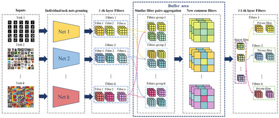
Figure 1.
An overview of the proposed method. For k incrementally added networks {Net 1, Net 2, …, Net k} with identical architectures handling distinct tasks/datasets, the AP framework proceeds through three stages: (1) Applying structured pruning techniques to perform neuron pruning on well-trained multi-task networks, obtaining compact task-specific networks; (2) Selecting high-affinity filter pairs via similarity metrics and merging them into new, shareable filters; (3) Clustering shareable filters into a shared filter family, while low-affinity filters are preserved to maintain task-specific performance.
2. Related Work
Pruning for DNNs. Network pruning is a widely adopted technique in deep learning that aims to reduce model complexity by eliminating redundant or less significant parameters. Pruning methods can be broadly categorized into two types based on their architectural approach: unstructured and structured pruning. Unstructured pruning [15,32] involves removing individual weights from the neural network without any specific pattern or structure. Each parameter is evaluated independently, and those deemed less significant are set to zero. In contrast, structured pruning [33,34] removes entire structures such as neurons, filters, or channels. By eliminating these components, the network becomes more efficient, and the resulting sparse matrices are more amenable to hardware acceleration. Pruning methods compute importance scores to determine which parameters to remove. Common pruning criteria include magnitude-based [13,32], gradient-based [18,35], Hessian-based [15,36], connection sensitivity-based [16,37], etc. Beyond post-training pruning, the Lottery Ticket Hypothesis [38] suggests that within a randomly initialized network, there exists a subnetwork that, when trained in isolation, can reach comparable performance to the original network. SNIP [39] attempts to find an initial mask in a data-driven approach with one-shot pruning and uses this initial mask to guide parameter selection. These methods maintain a static network architecture throughout the training process. Other approaches, such as dynamic pruning methods [40,41], have been proposed. These methods adjust the pruning mask during training according to predefined criteria, enabling more flexible and efficient pruning strategies.
Pruning for GNNs. Graph neural networks (GNNs) exhibit unique computational patterns distinct from traditional DNNs, driven by their unstructured, large-scale sparse graph inputs and the reliance on sparse matrix operations. Despite extensive research on DNN pruning, GNN pruning remains understudied. Previous studies in GNNs have focused mainly on irregular weight pruning [22,23,24] to reduce the complexity and computational cost of networks. However, irregular sparsity patterns hinder hardware efficiency due to limited parallelism. To address this, PruneGNN [42] introduces an algorithm-architecture co-designed framework, which employs structured sparse training and SIMD-optimized kernels to resolve parallelism bottlenecks caused by irregular pruning on GPUs.
Pruning for Multi-task Learning. The purpose of multi-task pruning is to remove the redundancy existing in the networks during training, thus minimizing the computational cost. According to the implementation strategy, it can be briefly divided into the following two categories: (1) By forcing the merging of multiple single-task networks into a compact multi-task network. In such cases as in [43], authors propose to combine neurons in the hidden layer of well-trained deep neural networks layer-by-layer to form a compact MTL network. Although these methods can effectively alleviate redundancy between tasks, they ignore the ability to represent individual tasks. (2) Pruning the multi-task network directly using existing network pruning technologies. For example, in [44], authors propose using the norm to prune filters in a multi-task semantic segmentation network to reduce semantic redundancy. In [28], authors first utilize individual network pruning techniques to suppress redundancy in multi-task networks. Although these methods restrain the redundancy in multi-task networks, they also cause some damage to the accuracy. Recently, AdapMTL [45] introduced an adaptive pruning framework that dynamically adjusts pruning thresholds during training, co-optimizing the model weights and sparsity for each task. This approach improves task accuracy while achieving high sparsity. DiSparse [46], on the other hand, applies a disentangled pruning strategy, treating each task independently to effectively reduce redundancy and improve multi-task model compression without negatively impacting performance. However, both of these methods were primarily designed for static or predefined multi-task learning setups and may face challenges as tasks incrementally increase over time.
While these methods have made significant progress in reducing redundancy and improving the efficiency of multi-task models, pruning for continuous incremental multi-task DNNs remains an underexplored challenge. Specifically, in dynamic real-world environments, mobile systems may need to continuously add more related neural networks or combinations to handle various tasks. As these new tasks introduce additional network redundancy, the efficiency of the combined network may decrease, leading to potential trade-offs between inference speed and accuracy. This motivates our work. Unlike existing strategies, our AP framework explicitly considers the integration of incrementally added tasks into an existing multi-task model. We design an adaptive threshold selection strategy to capture similar filters between the incrementally added task networks and the existing multi-task network. These similar filters are then merged and aggregated into a shared filter family. In this way, our approach not only reduces inter-task redundancy but also facilitates knowledge transfer across tasks.
3. The Proposed Method
In this section, we propose a pruning aggregation scheme to solve the compression problem for consecutive incremental tasks. We first introduce the problem setting of incremental multi-tasking. Then, we will introduce our proposed method in detail.
3.1. Problem Statement
We will formally introduce the symbols and annotations in this section. Without loss of generality, we give two related trained networks, a and b, and simply combine them into a multi-task network. Suppose that the network has a total of L layers, where the number of input and output channels of the l-th layer are and , , and the filter size is k. We can then obtain a representation in layer l that is learned by the following multi-task network:
- (1)
- Specialized filters for task a, i.e., filters that are only relevant to task a, which are defined as .
- (2)
- Specialized filters for task b, i.e., filters that are only relevant to task b, which are defined as .
- (3)
- Filter families. That is, filters related to both task a and task b, which are defined as .
- (4)
- In a convolutional layer, each filter consists of convolutional kernels. The number of uncompressed convolutional kernels in the multi-task network is given by Equation (1), where and represent the number of kernels specific to task networks a and b, respectively, and represents the number of shared kernels. Based on the kernel-to-filter relation, the total number of filters (i.e., output channels) in the layer is
From the above conditions, our convolution operation at the l-th layer can be written as follows:
where the function represents the concatenation; and represent the output tensors of the network a and b in the l-th layer, respectively, and their size is . Here, M denotes the batch size, and is the spatial dimension of the output feature maps.
Since this paper deals with continuous incremental multi-task network compression scenarios, we assume continuous incremental k-task networks, where , …, are buffers between and tasks in layer l, which are used for compressing and storing filters. Our aim is to encourage the aggregation of as many similar filter pairs as possible at the lower layers between task networks and selective aggregation at higher layers. In this way, (i) aggregation can minimize the loss, and (ii) the filter family is constructed involving auxiliary training of individual tasks.
3.2. Individual Task Pruning
In this part, in order to facilitate the beneficial deployment of continuous incremental deep neural networks in the system, we need to perform operations on these networks, including individual task network pruning and compression between networks. Considering the excessive parameters existing in the individual network itself, we first prune the trained individual network to obtain a compact network as follows:
where represents the filters of the individual network and is the -norm.
3.3. Buffer Area Build
To achieve aggregation of similar filter pairs between networks, we build buffers between each convolution layer. Suppose that there are incremental tasks and the l-th layer parameters are . We construct the buffer, and the steps are as follows:
- 1.
- For buffer , we construct a mask of the same size as P to delete the shared filters:where represents the i-th position in the buffers of the j-th and m-th tasks, and represents the a-th position in the buffer of the n-th and j-th tasks. Notably, is a 1 vector when first aggregated.
- 2.
- Calculate the size of as follows:where represents the weight of the j-th task network in the l-th layer, and ⊙ is the Hadamard product.
- 3.
- Next, we capture similar filter pairs between tasks through a similarity measure as follows:where represents the i-th convolution kernel filters of the l-th layer of the task network, and denotes the cosine similarity between two filters.
- 4.
- Next, we need to aggregate similar filter pairs to obtain a shared filter family with a strong representation. Here, we set up a buffer consisting of P and B for the shared filter. P represents the position index of the filters common to the current iteration, initialized to an empty matrix. B represents the position of the current iteration shared filter, initialized to an empty matrix. Then, we introduce a Mask matrix M of size , which is used to represent the filter coordinates of the network a that need to be shared by the current iteration as follows:where v is the threshold; ∅ represents vacancy.
- 5.
- The position index of the shared filter can be expressed as follows:where represents the i-th row and m-th column of the similarity matrix S, and represents the i-th position of the location buffer of task j, .
- 6.
- The value of the shared filter after aggregation iswhere represents the i-th entry of the filter buffer for task j, . represents the result calculated in (1) for the parameters of the i-th position of the l-th layer of the task j network. represents the result calculated in (1) for the parameters of the -th position of the l-th layer of the task network.
3.4. Filter Update
After the weights are aggregated, since the structure of the network has changed, if you want to continue training the network, the weight transfer method will also change. When back-propagating, the update of the private core does not change, while the update of the shared core, when we obtain the gradients received by the two networks at the shared location , , that is, the update rule of B at any non-empty position i is as follows:
where and are the learning rates for the two tasks, respectively.
Therefore, the update rule of B at any non-empty position i is as follows:
3.5. Adaptive Learning Mechanism
In order to allow the model to compress adaptively, we design an adaptive threshold selection strategy as follows:
where is a learnable parameter, the sharing tendency of each filter, represents the sampling of the standard Gumbel distribution, where , ∼, and is a uniform distribution between 0 and 1, and is the temperature parameter, which decreases to 0 as the number of training epochs increases.
We hope to encourage sharing in the shallow network and selectively share in the deep network so the loss function of adaptive learning is
where represents the shared threshold of the l-th layer. The total loss function of the entire network can be written as follows:
where represents the loss for task k, and and are the balance coefficients.
4. Experiments
All experiments were conducted using PyTorch 2.1.0 on two 24 GB RTX 3090 GPUs from NVIDIA (Santa Clara, CA, USA). For semantic segmentation and classification tasks, we adopted the cross-entropy loss, while for surface normal prediction, we employed the negative cosine similarity between the normalized predictions and ground-truth normals. To ensure a fair comparison across different methods and to avoid the influence of pre-trained weights, all models were trained from scratch.
4.1. Performance on Uniform Task Groups
To validate the efficiency of our method in scenarios where tasks share similar input-output modalities, we performed experiments on four classification task groups (Exp. A–D). These experiments analyze how our pruning-aggregation framework balances parameter reduction and accuracy preservation when tasks vary in label spaces or feature distributions.
Datasets. we conduct experiments on six widely used image classification datasets, including Fashion-MNIST [47], MNIST [48], Office-Caltech (DSLR) [49], Office-Caltech (Webcam), Office-Caltech (Amazon), and Art [50].
Baseline. we use a model with random pruning, skipping the aggregation scheme, as our baseline model and conduct experiments separately using norm and cosine distance.
Experimental Settings. To comprehensively validate the effectiveness and generalization of the proposed method, we design four scenarios with increasing complexity in feature relationships, label consistency, and compatibility across model architectures. Experiments are conducted using different backbone networks (LeNet-5 [51], VGG-16 [52], ResNet-50 [53]) to ensure the method’s adaptability to diverse designs:
- Exp. A: independent labels with shared low-level features. We combine two classification tasks on Fashion-MNIST and MNIST. Both datasets use 28 × 28 grayscale images, sharing similar low-level feature spaces (e.g., edge and texture patterns), but their label spaces are semantically independent (clothing vs. digits). LeNet-5 is used as a lightweight baseline to focus on task-specific learning.
- Exp. B: aligned labels with domain-Specific features. This scenario involves two classification tasks on the Office-Caltech Webcam (low-resolution images with environmental noise) and Amazon (high-resolution product images) subsets. While the label spaces are fully aligned, the feature distributions exhibit significant domain shifts. We adopt VGG-16 to evaluate the compatibility with classical deep CNNs lacking residual connections.
- Exp. C: architecture compatibility validation. Using the same tasks as Exp. B (Webcam and Amazon), we replace VGG-16 with ResNet-50 to evaluate the method’s performance on modern architectures with residual connections, explicitly verifying its adaptability to advanced network designs.
- Exp. D: partial label alignment with mixed feature domains and incremental tasks. Building on Exp. C, Exp. D extends this setup by adding two more datasets: Office-Caltech DSLR and the Art dataset. This extension introduces a more complex scenario with heterogeneous feature spaces (natural images vs. paintings) and partially overlapping labels (e.g., shared “chair” category in Office-Caltech vs. unique art categories). We build upon the multi-task network trained on the webcam and Amazon domains in Experiment C. Subsequently, we incrementally introduce two single-task networks for the DSLR and Art in a predefined order. The tasks are added one by one, enabling us to evaluate the scalability and effectiveness of our method in a continuous incremental learning setting. This experiment further validates our method’s adaptability to modern architectures with residual connections while handling the increased complexity introduced by new tasks with mixed feature domains and label alignments.
Evaluation Metrics and Loss Functions. We use classification accuracy as the primary evaluation metric for both individual tasks and multi-task combinations. In multi-task scenarios, accuracy reflects the average performance across all tasks. To assess the efficiency of our method, we also consider parameters (in millions, M) and FLOPs (floating-point operations, ), which indicate the model’s computational complexity and memory usage. Our method is optimized via a multi-task cross-entropy loss combined with an adaptive threshold regularization term (Equation (15)).
Experiment Results. By effectively pruning redundant filters, our method demonstrates robust performance in multi-task learning scenarios while preserving task-specific accuracy. Moreover, we extended our experiments to different model architectures to assess the model-agnostic nature of our method.
- Results on Exp. A: As shown in Table 1, tasks with independent labels but shared low-level features (Fashion-MNIST and MNIST) demonstrate that our method effectively aggregates filters, preserving task-specific features while reducing redundancy. This leads to improved accuracy and efficiency.
 Table 1. Exp. A. Experiments on Fashion-MNIST (A) and MNIST (B); the network used is LeNet-5. is pruned using the norm, and is pruned using cosine distance.
 - Results on Exp. B and C: As shown in Table 2 and Table 3, the results on both VGG-16 (Exp. B) and ResNet-50 (Exp. C) show similar trends in accuracy improvement and parameter reduction. Across both VGG-16 (Exp. B) and ResNet-50 (Exp. C), our method consistently demonstrates improvements in accuracy and reductions in parameters. Moreover, we observe that pruning slightly outperforms cosine pruning in terms of accuracy in ResNet-50, while cosine pruning results in marginally better parameter reduction. The results indicate that our approach is versatile and effective in handling domain-specific features with aligned labels, regardless of the underlying model architecture. These findings confirm that our method is capable of generalizing across different network designs while maintaining high performance and reducing computational overhead. It is also worth noting that Experiment B is designed to evaluate the model’s robustness to task feature distribution shifts, as it involves different domains in the Office-Caltech dataset. The consistent improvements achieved in this setting further demonstrate the generalization capability of our approach under distributional changes across tasks.
Table 2. Exp. B. Experiments on Webcam (A) and Amazon (B); the network used is VGG-16. is pruned using norm, and is pruned using cosine distance.
Table 3. Exp. C. Experiments on Webcam (A) and Amazon (B); the network used is ResNet-50. is pruned using norm, and is pruned using cosine distance.
- Results on Exp. D: As shown in Table 4, we evaluate a more complex scenario with four tasks, where partial label alignment and mixed feature domains are introduced. Our method maintains 87.33% accuracy while reducing parameters by 41.7%. This result demonstrates that, even with the increasing complexity of tasks and heterogeneity in label spaces, our method efficiently prunes redundant parameters. This highlights the effectiveness of our approach in maintaining task-specific accuracy while adapting to the addition of new tasks in a multi-task, incremental learning environment.
Table 4. Exp. D. Experiments on Webcam (A), Amazon (B), DSLR (C), and Art (D); the network used is ResNet-50. is pruned using norm, and is pruned using cosine distance.
4.2. Performance on Diverse Task Groups
To further verify the generalizability of our method in real-world applications, we evaluate it on a diverse task group containing both classification (semantic segmentation) and regression (depth estimation, surface normal) tasks.
Datasets: We conduct the experiments on a popular multi-task dataset: NYU-v2 [54]. The NYU-v2 dataset is composed of RGB-D indoor scene images and covers three tasks: 13-class semantic segmentation, depth estimation, and surface normal prediction.
Evaluation Metrics and Loss Functions: We use different evaluation metrics for each task. On the NYUv2 dataset, there are a total of three tasks. For semantic segmentation, we employ the mean Intersection over Union (mIoU) and Pixel Accuracy (Pixel Acc) as our primary evaluation metrics and use cross-entropy to calculate the loss. Surface normal prediction uses the inverse of cosine similarity between the normalized prediction and ground truth and is performed using mean and median angle distances between the prediction and the ground truth. We also report the percentage of pixels whose prediction is within the angles of 11.25°, 22.5°, and 30° to the ground truth. Depth estimation utilizes the L1 loss, with the absolute and relative errors between the prediction and ground truth being calculated. Again, we also present the relative difference between the prediction and ground truth by calculating the percentage of within the thresholds of 1.25, , and .
Baselines For Comparison: For MTL methods, we compare our work with Cross-Stitch [55], Sluice [56], and DEN [57]. We report their performance on the semantic segmentation and surface normal prediction tasks.
For pruning methods, we compare our work with LTH [58], IMP [13], SNIP [39], DiSparse [46], and AdapMTL [45]. For LTH, IMP, SNIP, and DiSparse, we follow the same experimental setup as AdapMTL. For AdapMTL, we directly use the official implementation provided by the authors from GitHub.
We use the same backbone model and maintain consistent sparsity levels across all pruning methods for a fair comparison. Our method adapts pruning based on specific threshold values, typically achieving a sparsity level between 30% and 40%. For clarity and consistency, we report the evaluation results at a sparsity level of 30%. We utilize Deeplab-ResNet34 [59] as the backbone model. The task-specific heads are implemented using the Atrous Spatial Pyramid Pooling (ASPP) architecture, which is widely adopted for pixel-wise prediction tasks.
Experiment Results: We present the comparison results with MTL methods and state-of-the-art pruning methods on the NYU-V2 dataset in Table 5. Overall, our method significantly outperforms existing pruning approaches and even non-pruning methods, such as Cross-Stitch, across most metrics. In terms of pruning methods, unlike methods like SNIP, which relies on single-batch gradient-based pruning and irreversibly damages shared low-level features critical for multi-task correlations, or LTH, which over-prioritizes task-specific heads at the expense of backbone sparsity, our framework dynamically constructs filter families to preserve cross-task geometric features such as edge and texture detectors. This contrasts with IMP’s iterative pruning-retraining cycles that incur significant computational overhead.
Table 5.
Comparison with several MTL methods and state-of-the-art pruning methods on the NYU-V2 [54] dataset using the Deeplab-ResNet34 [59] backbone. Bold indicates the best performance, ↑ indicates that larger values are better, and ↓ indicates that smaller values are better.
While DiSparse enforces unanimous pruning decisions across tasks to ensure compatibility, its rigidity limits parameter efficiency and fails to adapt to incremental task additions. AdapMTL, though adaptive in balancing sparsity between shared backbones and task heads through component-wise thresholds, assumes a static task configuration and cannot dynamically integrate new tasks. Our approach uniquely bridges these gaps by combining adaptive filter similarity clustering with buffer-driven layer-wise thresholds. By aggregating compatible filters into shared families and maintaining task-specific buffers for incremental updates, we minimize redundancy without sacrificing task-critical features. This enables seamless integration of new tasks while preserving backbone integrity, a capability absent in both DiSparse’s unanimity-driven pruning and AdapMTL’s fixed component optimization.
4.3. Analysis
Effectiveness of Pruning and Aggregation. Our experiments demonstrate that the AP framework effectively reduces the parameter footprint of multi-task networks while preserving task-specific accuracy. By pruning redundant filters within individual task networks and aggregating similar filters across tasks, the method achieves a balance between efficiency and generalization. As shown by previous experiments, this finding is consistently validated across different evaluations. AP significantly compresses the model size without degrading performance, confirming that critical knowledge is effectively retained and shared across tasks.
The class activation maps (CAMs) in Figure 2 further validate this design. Even after pruning, the network consistently focuses on the critical parts of the image, such as the handle of a backpack or the texture of a helmet, demonstrating that task-specific discriminability is preserved. This underscores AP’s ability to maintain task-specific performance while enabling cross-task knowledge transfer, enhancing generalization of every single network.
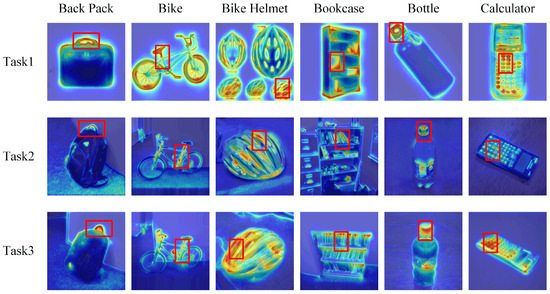
Figure 2.
Class activation maps (CAM) for three tasks, each corresponding to a different sub-dataset of the Office-Caltech dataset, after pruning using our method. The red bounding boxes highlight the regions the pruned model focuses on, which represent the key features that define each image’s category.
Sharing in Shallow and Deep Layers. A key innovation of our method lies in its adaptive sharing strategy across network layers. Figure 3 illustrates the filter sharing ratio across layers in the Deeplab-ResNet34 model that was trained on the NYUv2, revealing that shallow layers exhibit higher sharing proportions compared with deeper layers. This aligns with the intuition that early layers capture generic low-level features (e.g., edges, textures), which are naturally reusable across tasks. In contrast, deeper layers encode task-specific semantics, necessitating selective sharing to avoid interference. Through its adaptive learning mechanism, AP can effectively minimize redundancy across tasks while ensuring that each task maintains its specialized features.
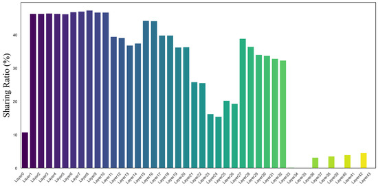
Figure 3.
Filter sharing ratio across layers in Deeplab-ResNet34, trained on the NYUv2 dataset. This figure illustrates how filter sharing is distributed across different layers of the network.
Shared Feature Representation. The success of our method is largely due to the shared feature representations, which are achieved through the aggregation of similar filters. We trained three VGG-19 networks using the Office31 dataset, corresponding to three tasks. Prior to applying our filter-sharing method, we visualized the similarity of the first convolution layer filters between Task 1 and Task 2. As shown in Figure 4, the similarity matrix between Task 1 and Task 2 reveals that there are many filters between tasks that share a high degree of similarity, especially along the diagonal, meaning that the filters at the same positions across tasks are highly similar. This high similarity suggests that, despite the filters coming from different tasks, the filters at these positions have learned similar features. Furthermore, we visualized 10 pairs of convolution kernels selected for sharing from the fifth convolution layer of Task 1 and Task 2 networks, as shown in Figure 5. The high similarity of certain filters between tasks further supports our redundancy reduction strategy. By sharing these highly similar filters, we can effectively reduce redundancy while preserving task-specific features and discriminative power.
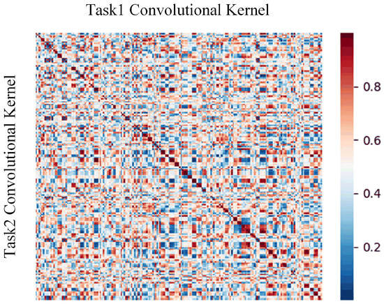
Figure 4.
Similarity matrix between Task 1 and Task 2 in the first convolution layer showing the high similarity of filters at the same positions across tasks.
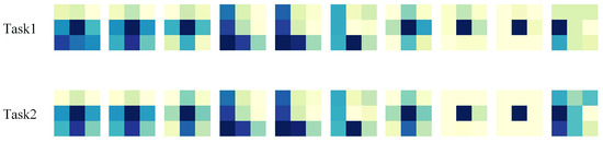
Figure 5.
Ten pairs of convolution kernels selected for sharing from the fifth convolution layer of Task 1 and Task 2.
Impact of Continuous Incremental Tasks: A hallmark of AP is its robustness in handling continuous task increments. As shown in Exp. D (Table 4), the method adapts seamlessly to newly added tasks without significant performance degradation. This adaptability stems from two mechanisms: (1) Buffer-driven redundancy suppression: task-specific buffers isolate incremental redundancy, preventing interference with existing knowledge. (2) Dynamic filter updates: shared filter families are incrementally refined during backpropagation, ensuring stable convergence across tasks. By minimizing redundancy between tasks and maintaining high task-specific accuracy, the AP method ensures that performance does not deteriorate as new tasks are added, which is critical for real-world applications requiring continuous learning and adaptation.
4.4. Ablation Studies
To assess the effectiveness of each component of our proposed method, we conducted ablation studies. For example, the ‘random aggregation’ model tests the importance of filter similarity in improving task performance, while the ‘no filter update’ model isolates the effect of dynamic filter refinement. These comparisons are crucial for understanding the contributions of individual mechanisms to the overall performance. We tested three variations: the model with random aggregation (Section 3.3), where instead of aggregating filters based on similarity, the filters were randomly aggregated to evaluate whether similarity-based aggregation is crucial for task performance; the model with static filter update (Section 3.4), where the shared filters were statically fused using an average method; and the model without an adaptive learning mechanism (Section 3.5), where a static threshold of 0.5 was used for pruning instead of the adaptive threshold mechanism. All ablation experiments were conducted with a uniform sparsity rate of 35%. The results showed that using static filter updates, random aggregation, and a fixed threshold all led to performance drops, highlighting the significance of each component in the proposed method.
We additionally compared with three full individual networks separately trained on each task. As shown in Table 6, under the 35% sparsity setting, the full networks show no performance advantage over our method, even underperforming the simplified variants on tasks like semantic segmentation and surface normal estimation. This empirically validates the inherent redundancy in over-parameterized networks and AP’s efficacy in eliminating such redundancy through systematic filter aggregation.
Table 6.
Ablations on NYU-v2. Bold indicates the best performance, ↑ indicates that larger values are better, and ↓ indicates that smaller values are better.
5. Conclusions
In this paper, we propose AP, a novel pruning and aggregation method for continuous incremental multi-task learning. Our approach efficiently reduces the parameter size of multi-task networks by pruning redundant filters and aggregating similar filters across tasks. Additionally, AP incorporates an adaptive learning mechanism that adjusts filter-sharing strategies based on task similarities, effectively minimizing redundancy while maintaining task-specific accuracy. Another key feature of our method is the dynamic filter update mechanism, which ensures that shared filter families are incrementally refined during training to maintain model performance across tasks. We validate the effectiveness of our method through extensive experiments across multiple datasets and architectures, demonstrating its superiority in parameter reduction and efficiency over existing pruning and multi-task learning methods. Furthermore, the architecture-agnostic nature of AP makes it extensible to multi-task GNNs, which we will prioritize extending in future work.
Author Contributions
Conceptualization, L.L., F.C. and Q.F.; methodology, L.L. and Q.F.; software, F.C.; validation, L.L. and F.C.; formal analysis, F.C.; investigation, L.L. and F.C.; resources, Q.F.; data curation, F.C.; writing—original draft, L.L.; writing—review and editing, L.L., F.C. and J.X.; visualization, L.L. and F.C.; supervision, J.X.; project administration, Q.F.; funding acquisition, J.X. All authors have read and agreed to the published version of the manuscript.
Funding
This work has been supported by the National Natural Science Foundation of China under grants [No. 62366008] and [No. 61966005].
Data Availability Statement
The data instances for this study are available at https://drive.google.com/file/d/11pWuQXMFBNMIIB4VYMzi9RPE-nMOBU8g/view?pli=1, accessed on 23 October 2024.
Conflicts of Interest
Quan Feng was employed by Hunan Vanguard Group Corporation Limited. The remaining authors declare that the research was conducted in the absence of any commercial or financial relationships that could be construed as a potential conflict of interest.
References
- Zhan, J.; Luo, Y.; Guo, C.; Wu, Y.; Meng, J.; Liu, J. YOLOPX: Anchor-free multi-task learning network for panoptic driving perception. Pattern Recognit. 2024, 148, 110152. [Google Scholar] [CrossRef]
- Tapu, R.; Mocanu, B.; Zaharia, T. Wearable assistive devices for visually impaired: A state of the art survey. Pattern Recognit. Lett. 2020, 137, 37–52. [Google Scholar] [CrossRef]
- Meshram, V.V.; Patil, K.; Meshram, V.A.; Shu, F.C. An astute assistive device for mobility and object recognition for visually impaired people. IEEE Trans. Hum.-Mach. Syst. 2019, 49, 449–460. [Google Scholar] [CrossRef]
- Krishna, S.; Little, G.; Black, J.; Panchanathan, S. A wearable face recognition system for individuals with visual impairments. In Proceedings of the 7th International ACM SIGACCESS Conference on Computers and Accessibility, Baltimore, MD, USA, 9–12 October 2005; pp. 106–113. [Google Scholar]
- Poggi, M.; Mattoccia, S. A wearable mobility aid for the visually impaired based on embedded 3D vision and deep learning. In Proceedings of the 2016 IEEE Symposium on Computers and Communication (ISCC), Messina, Italy, 27–30 June 2016; IEEE: Piscataway, NJ, USA, 2016; pp. 208–213. [Google Scholar]
- Schmidhuber, J. Deep learning in neural networks: An overview. Neural Netw. 2015, 61, 85–117. [Google Scholar]
- Samek, W.; Montavon, G.; Lapuschkin, S.; Anders, C.J.; Müller, K.R. Explaining deep neural networks and beyond: A review of methods and applications. Proc. IEEE 2021, 109, 247–278. [Google Scholar] [CrossRef]
- Li, Z.; Liu, F.; Yang, W.; Peng, S.; Zhou, J. A survey of convolutional neural networks: Analysis, applications, and prospects. IEEE Trans. Neural Netw. Learn. Syst. 2021, 33, 6999–7019. [Google Scholar] [CrossRef]
- Jiang, W.; Luo, J. Graph neural network for traffic forecasting: A survey. Expert Syst. Appl. 2022, 207, 117921. [Google Scholar] [CrossRef]
- Sharma, K.; Lee, Y.C.; Nambi, S.; Salian, A.; Shah, S.; Kim, S.W.; Kumar, S. A survey of graph neural networks for social recommender systems. ACM Comput. Surv. 2024, 56, 265. [Google Scholar] [CrossRef]
- Liu, J.; Yang, C.; Lu, Z.; Chen, J.; Li, Y.; Zhang, M.; Bai, T.; Fang, Y.; Sun, L.; Yu, P.S.; et al. Towards graph foundation models: A survey and beyond. arXiv 2023, arXiv:2310.11829. [Google Scholar]
- Wu, L.; He, X.; Wang, X.; Zhang, K.; Wang, M. A survey on accuracy-oriented neural recommendation: From collaborative filtering to information-rich recommendation. IEEE Trans. Knowl. Data Eng. 2022, 35, 4425–4445. [Google Scholar] [CrossRef]
- Han, S.; Mao, H.; Dally, W.J. Deep compression: Compressing deep neural networks with pruning, trained quantization and huffman coding. arXiv 2015, arXiv:1510.00149. [Google Scholar]
- Zhuang, W.; Wen, Y.; Lyu, L.; Zhang, S. MAS: Towards resource-efficient federated multiple-task learning. In Proceedings of the 2023 IEEE/CVF International Conference on Computer Vision (ICCV), Paris, France, 1–6 October 2023; pp. 23414–23424. [Google Scholar]
- LeCun, Y.; Denker, J.; Solla, S. Optimal brain damage. In Advances in Neural Information Processing Systems; MIT Press: Cambridge, MA, USA, 1989; Volume 2, pp. 598–605. [Google Scholar]
- Su, J.; Chen, Y.; Cai, T.; Wu, T.; Gao, R.; Wang, L.; Lee, J.D. Sanity-checking pruning methods: Random tickets can win the jackpot. In Advances in Neural Information Processing Systems; MIT Press: Cambridge, MA, USA, 2020; Volume 33, pp. 20390–20401. [Google Scholar]
- Sanh, V.; Wolf, T.; Rush, A. Movement pruning: Adaptive sparsity by fine-tuning. In Advances in Neural Information Processing Systems; MIT Press: Cambridge, MA, USA, 2020; Volume 33, pp. 20378–20389. [Google Scholar]
- Molchanov, D.; Ashukha, A.; Vetrov, D. Variational dropout sparsifies deep neural networks. In Proceedings of the 34th International Conference on Machine Learning, Sydney, Australia, 6–11 August 2017; pp. 2498–2507. [Google Scholar]
- Chen, Y.; Zheng, B.; Zhang, Z.; Wang, Q.; Shen, C.; Zhang, Q. Deep learning on mobile and embedded devices: State-of-the-art, challenges, and future directions. ACM Comput. Surv. (CSUR) 2020, 53, 84. [Google Scholar] [CrossRef]
- Molchanov, P.; Tyree, S.; Karras, T.; Aila, T.; Kautz, J. Pruning convolutional neural networks for resource efficient inference. arXiv 2016, arXiv:1611.06440. [Google Scholar]
- Kuutti, S.; Bowden, R.; Jin, Y.; Barber, P.; Fallah, S. A survey of deep learning applications to autonomous vehicle control. IEEE Trans. Intell. Transp. Syst. 2020, 22, 712–733. [Google Scholar] [CrossRef]
- Peng, H.; Gurevin, D.; Huang, S.; Geng, T.; Jiang, W.; Khan, O.; Ding, C. Towards sparsification of graph neural networks. In Proceedings of the 2022 IEEE 40th International Conference on Computer Design (ICCD), Olympic Valley, CA, USA, 23–26 October 2022; IEEE: Piscataway, NJ, USA, 2022; pp. 272–279. [Google Scholar]
- Luo, Y.; Behnam, P.; Thorat, K.; Liu, Z.; Peng, H.; Huang, S.; Zhou, S.; Khan, O.; Tumanov, A.; Ding, C.; et al. Codg-reram: An algorithm-hardware co-design to accelerate semi-structured gnns on reram. In Proceedings of the 2022 IEEE 40th International Conference on Computer Design (ICCD), Olympic Valley, CA, USA, 23–26 October 2022; IEEE: Piscataway, NJ, USA, 2022; pp. 280–289. [Google Scholar]
- Chen, T.; Sui, Y.; Chen, X.; Zhang, A.; Wang, Z. A unified lottery ticket hypothesis for graph neural networks. In Proceedings of the 38th International Conference on Machine Learning, Virtual Event, 18–24 July 2021; pp. 1695–1706. [Google Scholar]
- Skarding, J.; Gabrys, B.; Musial, K. Foundations and modeling of dynamic networks using dynamic graph neural networks: A survey. IEEE Access 2021, 9, 79143–79168. [Google Scholar] [CrossRef]
- Chou, Y.M.; Chan, Y.M.; Lee, J.H.; Chiu, C.Y.; Chen, C.S. Unifying and merging well-trained deep neural networks for inference stage. arXiv 2018, arXiv:1805.04980. [Google Scholar]
- Dellinger, F.; Boulay, T.; Barrenechea, D.M.; El-Hachimi, S.; Leang, I.; Bürger, F. Multi-task network pruning and embedded optimization for real-time deployment in adas. arXiv 2021, arXiv:2101.07831. [Google Scholar]
- He, X.; Gao, D.; Zhou, Z.; Tong, Y.; Thiele, L. Pruning-aware merging for efficient multitask inference. In Proceedings of the 27th ACM SIGKDD Conference on Knowledge Discovery & Data Mining, Virtual Event, 14–18 August 2021; pp. 585–595. [Google Scholar]
- Ye, H.; Zhang, B.; Chen, T.; Fan, J.; Wang, B. Performance-aware approximation of global channel pruning for multitask cnns. IEEE Trans. Pattern Anal. Mach. Intell. 2023, 45, 10267–10284. [Google Scholar] [CrossRef]
- He, Y.; Liu, P.; Zhu, L.; Yang, Y. Filter pruning by switching to neighboring CNNs with good attributes. IEEE Trans. Neural Netw. Learn. Syst. 2022, 34, 8044–8056. [Google Scholar] [CrossRef]
- Kanakis, M.; Bruggemann, D.; Saha, S.; Georgoulis, S.; Obukhov, A.; Van Gool, L. Reparameterizing convolutions for incremental multi-task learning without task interference. In Computer Vision—ECCV 2020: 16th European Conference, Glasgow, UK, 23–28 August 2020, Proceedings, Part XX; Springer: Cham, Switzerland, 2020; pp. 689–707. [Google Scholar]
- Han, S.; Pool, J.; Tran, J.; Dally, W. Learning both weights and connections for efficient neural network. In Advances in Neural Information Processing Systems; MIT Press: Cambridge, MA, USA, 2015; Volume 28. [Google Scholar]
- Liu, Y.; Chen, K.; Liu, C.; Qin, Z.; Luo, Z.; Wang, J. Structured knowledge distillation for semantic segmentation. In Proceedings of the 2019 IEEE/CVF Conference on Computer Vision and Pattern Recognition (CVPR), Long Beach, CA, USA, 15–20 June 2019; pp. 2604–2613. [Google Scholar]
- Garg, S.; Zhang, L.; Guan, H. Structured pruning for multi-task deep neural networks. In Proceedings of the 2024 IEEE 7th International Conference on Multimedia Information Processing and Retrieval (MIPR), San Jose, CA, USA, 7–9 August 2024; IEEE: Piscataway, NJ, USA, 2024; pp. 260–266. [Google Scholar]
- Molchanov, P.; Mallya, A.; Tyree, S.; Frosio, I.; Kautz, J. Importance estimation for neural network pruning. In Proceedings of the 2019 IEEE/CVF Conference on Computer Vision and Pattern Recognition (CVPR), Long Beach, CA, USA, 15–20 June 2019; pp. 11264–11272. [Google Scholar]
- Hassibi, B.; Stork, D. Second order derivatives for network pruning: Optimal brain surgeon. In Advances in Neural Information Processing Systems; MIT Press: Cambridge, MA, USA, 1992; Volume 5. [Google Scholar]
- Luo, J.H.; Wu, J. Neural network pruning with residual-connections and limited-data. In Proceedings of the 2020 IEEE/CVF Conference on Computer Vision and Pattern Recognition (CVPR), Seattle, WA, USA, 13–19 June 2020; pp. 1458–1467. [Google Scholar]
- Malach, E.; Yehudai, G.; Shalev-Schwartz, S.; Shamir, O. Proving the lottery ticket hypothesis: Pruning is all you need. In Proceedings of the 37th International Conference on Machine Learning, Virtual Event, 13–18 July 2020; pp. 6682–6691. [Google Scholar]
- Lee, N.; Ajanthan, T.; Torr, P.H. Snip: Single-shot network pruning based on connection sensitivity. arXiv 2018, arXiv:1810.02340. [Google Scholar]
- Park, J.H.; Kim, Y.; Kim, J.; Choi, J.Y.; Lee, S. Dynamic structure pruning for compressing CNNs. In Proceedings of the Thirty-Seventh AAAI Conference on Artificial Intelligence, Washington, DC, USA, 7–14 February 2023; Volume 37, pp. 9408–9416. [Google Scholar]
- Chen, J.; Chen, S.; Pan, S.J. Storage efficient and dynamic flexible runtime channel pruning via deep reinforcement learning. In Advances in Neural Information Processing Systems; MIT Press: Cambridge, MA, USA, 2020; Volume 33, pp. 14747–14758. [Google Scholar]
- Gurevin, D.; Shan, M.; Huang, S.; Hasan, M.A.; Ding, C.; Khan, O. Prunegnn: Algorithm-architecture pruning framework for graph neural network acceleration. In Proceedings of the 2024 IEEE International Symposium on High-Performance Computer Architecture (HPCA), Edinburgh, UK, 2–6 March 2024; IEEE: Piscataway, NJ, USA, 2024; pp. 108–123. [Google Scholar]
- He, X.; Zhou, Z.; Thiele, L. Multi-task zipping via layer-wise neuron sharing. In Advances in Neural Information Processing Systems; MIT Press: Cambridge, MA, USA, 2018; Volume 31. [Google Scholar]
- Chen, X.; Zhang, Y.; Wang, Y. MTP: Multi-task pruning for efficient semantic segmentation networks. In Proceedings of the 2022 IEEE International Conference on Multimedia and Expo (ICME), Taipei, Taiwan, 18–22 July 2022; IEEE: Piscataway, NJ, USA, 2022; pp. 1–6. [Google Scholar]
- Xiang, M.; Tang, J.; Yang, Q.; Guan, H.; Liu, T. AdapMTL: Adaptive Pruning Framework for Multitask Learning Model. In Proceedings of the 32nd ACM International Conference on Multimedia, Melbourne, Australia, 28 October–1 November 2024; pp. 5121–5130. [Google Scholar]
- Sun, X.; Hassani, A.; Wang, Z.; Huang, G.; Shi, H. Disparse: Disentangled sparsification for multitask model compression. In Proceedings of the 2022 IEEE/CVF Conference on Computer Vision and Pattern Recognition (CVPR), New Orleans, LA, USA, 18–24 June 2022; pp. 12382–12392. [Google Scholar]
- Xiao, H.; Rasul, K.; Vollgraf, R. Fashion-mnist: A novel image dataset for benchmarking machine learning algorithms. arXiv 2017, arXiv:1708.07747. [Google Scholar]
- Deng, L. The mnist database of handwritten digit images for machine learning research [best of the web]. IEEE Signal Process. Mag. 2012, 29, 141–142. [Google Scholar] [CrossRef]
- Gong, B.; Shi, Y.; Sha, F.; Grauman, K. Geodesic flow kernel for unsupervised domain adaptation. In Proceedings of the 2012 IEEE Conference on Computer Vision and Pattern Recognition, Providence, RI, USA, 16–21 June 2012; IEEE: Piscataway, NJ, USA, 2012; pp. 2066–2073. [Google Scholar]
- Tan, W.R.; Chan, C.S.; Aguirre, H.E.; Tanaka, K. Improved ArtGAN for conditional synthesis of natural image and artwork. IEEE Trans. Image Process. 2018, 28, 394–409. [Google Scholar] [CrossRef] [PubMed]
- LeCun, Y.; Bottou, L.; Bengio, Y.; Haffner, P. Gradient-based learning applied to document recognition. Proc. IEEE 1998, 86, 2278–2324. [Google Scholar] [CrossRef]
- Simonyan, K.; Zisserman, A. Very deep convolutional networks for large-scale image recognition. arXiv 2014, arXiv:1409.1556. [Google Scholar]
- He, K.; Zhang, X.; Ren, S.; Sun, J. Deep residual learning for image recognition. In Proceedings of the 2016 IEEE Conference on Computer Vision and Pattern Recognition (CVPR), Las Vegas, NV, USA, 27–30 June 2016; pp. 770–778. [Google Scholar]
- Silberman, N.; Hoiem, D.; Kohli, P.; Fergus, R. Indoor segmentation and support inference from rgbd images. In Computer Vision—ECCV 2012, In Proceedings of the 12th European Conference on Computer Vision, Florence, Italy, 7–13 October 2012. Proceedings, Part V; Springer: Berlin/Heidelberg, Germany, 2012; pp. 746–760. [Google Scholar]
- Misra, I.; Shrivastava, A.; Gupta, A.; Hebert, M. Cross-stitch networks for multi-task learning. In Proceedings of the 2016 IEEE Conference on Computer Vision and Pattern Recognition (CVPR), Las Vegas, NV, USA, 27–30 June 2016; pp. 3994–4003. [Google Scholar]
- Ruder, S.; Bingel, J.; Augenstein, I.; Søgaard, A. Latent multi-task architecture learning. In Proceedings of the Thirty-Third AAAI Conference on Artificial Intelligence, Honolulu, HI, USA, 27 January–1 February 2019; Volume 33, pp. 4822–4829. [Google Scholar]
- Ahn, C.; Kim, E.; Oh, S. Deep elastic networks with model selection for multi-task learning. In Proceedings of the 2019 IEEE/CVF International Conference on Computer Vision (ICCV), Seoul, Republic of Korea, 27 October–2 November 2019; pp. 6529–6538. [Google Scholar]
- Frankle, J.; Dziugaite, G.K.; Roy, D.; Carbin, M. Linear mode connectivity and the lottery ticket hypothesis. In Proceedings of the 37th International Conference on Machine Learning, Vienna, Austria, 12–18 July 2020; pp. 3259–3269. [Google Scholar]
- Chen, L.C.; Papandreou, G.; Kokkinos, I.; Murphy, K.; Yuille, A.L. Deeplab: Semantic image segmentation with deep convolutional nets, atrous convolution, and fully connected crfs. IEEE Trans. Pattern Anal. Mach. Intell. 2017, 40, 834–848. [Google Scholar] [CrossRef]
Disclaimer/Publisher’s Note: The statements, opinions and data contained in all publications are solely those of the individual author(s) and contributor(s) and not of MDPI and/or the editor(s). MDPI and/or the editor(s) disclaim responsibility for any injury to people or property resulting from any ideas, methods, instructions or products referred to in the content. |
© 2025 by the authors. Licensee MDPI, Basel, Switzerland. This article is an open access article distributed under the terms and conditions of the Creative Commons Attribution (CC BY) license (https://creativecommons.org/licenses/by/4.0/).