Objective Framework for Bayesian Inference in Multicomponent Pareto Stress–Strength Model Under an Adaptive Progressive Type-II Censoring Scheme

Abstract

This study introduces an objective Bayesian approach for estimating the reliability of a multicomponent stress–strength model based on the Pareto distribution under an adaptive progressive Type-II censoring scheme. The proposed method is developed within a Bayesian framework, utilizing a reference prior with partial information to improve the accuracy of point estimation and to ensure the construction of a credible interval for uncertainty assessment. This approach is particularly useful for addressing several limitations of a widely used likelihood-based approach in estimating the multicomponent stress–strength reliability under the Pareto distribution. For instance, in the likelihood-based method, the asymptotic variance–covariance matrix may not exist due to certain constraints. This limitation hinders the construction of an approximate confidence interval for assessing the uncertainty. Moreover, even when an approximate confidence interval is obtained, it may fail to achieve nominal coverage levels in small sample scenarios. Unlike the likelihood-based method, the proposed method provides an efficient estimator across various criteria and constructs a valid credible interval, even with small sample sizes. Extensive simulation studies confirm that the proposed method yields reliable and accurate inference across various censoring scenarios, and a real data application validates its practical utility. These results demonstrate that the proposed method is an effective alternative to the likelihood-based method for reliability inference in the multicomponent stress–strength model based on the Pareto distribution under an adaptive progressive Type-II censoring scheme.

1. Introduction

Reliability assessment plays a crucial role in various industrial and research disciplines, particularly in systems composed of multiple interacting components or entities. The operational integrity of such systems fundamentally depends on the ability of individual components to endure externally applied stress. This evaluation is mathematically modeled using a stress–strength model, which has extensive applications across diverse domains. In its most basic form, the stress–strength model quantifies the probability that the strength $\left(X\right)$ of a component exceeds the applied stress $\left(Y\right)$, defining the reliability metric as $R=P(X>Y)$. However, real-world systems generally involve multiple interacting components rather than a single one, forming multicomponent systems. In such systems, a subset of components must withstand the stress for the system to remain functional. This framework can be generalized as an s-out-of-k system, where $1\le s\le k$. Let $X_1,\dots ,X_k$ be independent and identically distributed strength variables with a cumulative distribution function (CDF) $F_X(·)$, and let Y be the common stress variable with the CDF $F_Y(·)$. Then, the reliability of a multicomponent system, introduced by Bhattacharyya and Johnson [1], is formulated as

$$\begin{array}{cc}\hfill R_{s,k}\left(\mathit{\varphi }\right)& =P\left(\mathrm{a}\mathrm{t} \mathrm{l}\mathrm{e}\mathrm{a}\mathrm{s}\mathrm{t} s \mathrm{o}\mathrm{f}(X_1,\dots ,X_k)\mathrm{e}\mathrm{x}\mathrm{c}\mathrm{e}\mathrm{e}\mathrm{d} Y\right)\hfill \\ \hfill & =\sum _{i=s}^k\left({\displaystyle \genfrac{}{}{0pt}{}{k}{i}}\right){\int }_{-\infty }^{\infty }{\left[1-F_X(t;{\mathit{\varphi }}_1)\right]}^i{\left[F_X(t;{\mathit{\varphi }}_1)\right]}^{k-i}d{F}_Y(t;{\mathit{\varphi }}_2),\hfill \end{array}$$

(1)

where $\mathit{\varphi }=\left({\mathit{\varphi }}_1,{\mathit{\varphi }}_2\right)$ denotes an unknown parameter vector, with ${\mathit{\varphi }}_1$ and ${\mathit{\varphi }}_2$ representing the parameters of $F_X(·)$ and $F_Y(·)$, respectively. The reliability framework of a multicomponent system extends beyond engineering applications and has found relevance in various other domains, including the following:

• Insurance: estimating the probability that a specified number of policyholders can withstand financial losses, thereby ensuring the stability of an insurance pool.
• Finance: assessing the resilience of financial institutions by modeling the possibility that a sufficient subset can withstand extreme market fluctuations.
• Climate risk assessment: estimating the probability that an adequate number of geographic regions can withstand large-scale natural disasters without triggering systemic collapse.
• Healthcare systems: determining whether a sufficient number of hospitals or intensive care units can absorb patient surges during public health crises, thereby maintaining overall system functionality.

Some researchers have explored different distributional assumptions for strength and stress variables to estimate the reliability of multicomponent stress–strength models. For instance, Wang et al. [2] employed likelihood-based and pivotal-based methods to analyze the reliability of a multicomponent stress–strength model, assuming the bathtub-shaped distribution. Similarly, Lio et al. [3] investigated the same estimation methods as Wang et al. [2] but within the framework of the Burr XII distribution. Jha et al. [4] analyzed the reliability of a multicomponent stress–strength model based on the unit generalized exponential distribution. They adopted both frequentist and Bayesian perspectives, and the frequentist methods included likelihood-based estimation, least squares, weighted least squares, and maximum product spacing approaches. Additionally, Jana and Bera [5] concentrated on interval estimation of the reliability of a multicomponent stress–strength model, assuming the inverse Weibull distribution.

Reliability estimation often involves censored data arising from experimental constraints or operational limitations. One of the most widely used censoring schemes (CSs) is the progressive Type-II (PT-II) CS, which allows the removal of surviving units during the experiment. However, despite its popularity, the PT-II CS may be inefficient due to a potentially long overall experimental duration. To overcome this issue, an adaptive PT-II (APT-II) CS has been proposed by Ng et al. [6], which adaptively adjusts the removal of surviving units based on a given time threshold T. This CS allows the experimenter to terminate the experiment as soon as possible once the experimental time exceeds a predetermined time T, ensuring that the total duration does not deviate much from the ideal time T. By doing so, it helps reduce both the total experiment time and associated costs. The efficiency of the APT-II CS has led to its application by various authors, such as Chen and Gui [7], Ateya et al. [8], and Dutta et al. [9].

This study focuses on estimating the reliability of a multicomponent stress–strength model, in which both strength and stress variables have the Pareto distribution under the APT-II CS. The Pareto distribution is particularly well suited for modeling heavy-tailed characteristics, which are commonly observed in empirical data across various domains. In fields such as insurance, finance, climate risk assessment, and healthcare economics, rare yet extreme events can significantly impact overall system behavior. Given its ability to accommodate such extreme-value phenomena, the Pareto distribution serves as a natural choice for stress–strength modeling in reliability analysis. However, a classical likelihood-based method often faces significant challenges when estimating the reliability of a multicomponent stress–strength model with Pareto-distributed variables under the APT-II CS. Specifically, the asymptotic variance–covariance matrix (AVCM) is not always well defined due to certain constraints. This limitation obstructs the construction of an approximate confidence interval (ACI), making it difficult for the likelihood-based method to assess the uncertainty in reliability estimation. Furthermore, even if the ACI is obtained, it may fail to achieve nominal coverage levels in small sample scenarios, resulting in unreliable inference. While the bootstrap method can be considered as an alternative for uncertainty quantification, it performs poorly when applied to the Pareto distribution under small sample conditions. This is because the maximum likelihood estimator (MLE) of the scale parameter is based on the first-order statistic, which is always greater than the true parameter value due to the lower-bound constraint imposed by the support of the distribution. In small samples, the estimation error becomes more substantial, leading to invalid inference.

To address these limitations, we develop an objective Bayesian approach using a reference prior with partial information, which retains the objectivity of traditional reference priors while enhancing both the stability of inference and the robustness of posterior estimation. By incorporating prior knowledge informed by the Fisher information matrix and systematically updating parameter uncertainty through the posterior distribution, the proposed framework facilitates the construction of a credible interval (CrI) for the multicomponent stress–strength reliability, effectively addressing the shortcomings of the likelihood-based method. The proposed approach not only enhances inference accuracy but also ensures valid CrI construction for the multicomponent stress–strength reliability from the Pareto distribution under the APT-II CS. These advantages are particularly prominent in small sample scenarios. In experiments involving censored data, practical constraints such as time and cost often result in inherently limited data availability. For this reason, statistical inference is frequently required under small sample conditions, which significantly compromises the applicability and performance of classical frequentist methods. In contrast, the proposed Bayesian approach offers stable and reliable inference across various applications and experimental settings with limited data.

The rest of this study is organized as follows: Section 2 describes the Pareto distribution and the APT-II CS used for modeling the multicomponent stress–strength reliability. Section 3 provides a likelihood-based approach within a frequentist framework, and Section 4 develops an objective Bayesian approach using a reference prior with partial information for estimating the multicomponent stress–strength reliability under the APT-II CS. Section 5 presents the results of a simulation study and real data analysis, and Section 6 concludes this study.

2. Model Description

2.1. Pareto Distribution

The probability density function (PDF) and CDF of a Pareto-distributed random variable X are given by

$$\begin{array}{cc}\hfill & f(x;\theta ,\lambda )=\lambda {\theta }^{\lambda }{x}^{-(\lambda +1)}\hfill \end{array}$$

and

$$\begin{array}{c}F(x;\theta ,\lambda )=1-{\left({\displaystyle \frac{\theta }{x}}\right)}^{\lambda },x>\theta ,\theta >0,\lambda >0,\hfill \end{array}$$

(2)

respectively, where $\theta$ denotes the scale parameter, and $\lambda$ denotes the shape parameter which is of primary importance both statistically and practically. In particular, the shape parameter $\lambda$ plays a fundamental role in defining the characteristics of the Pareto distribution, including the heaviness of its tail. This parameter directly influences the probability of extreme values, making it crucial in fields such as risk management, insurance, and financial modeling. A larger value of $\lambda$ results in a thinner tail, meaning that extreme events become less probable, whereas a smaller value of $\lambda$ implies a heavier tail, increasing the probability of rare but catastrophic occurrences. Furthermore, the existence of key moments depends on the shape parameter $\lambda$; specifically, the expectation of a Pareto-distributed variable exists only for $\lambda >1$, and its variance is finite only for $\lambda >2$. This dependency underscores the importance of accurately estimating the shape parameter $\lambda$ in decision-making processes related to risk assessment and reliability analysis.

For this reason, we assume distinct shape parameters for the strength and stress variables in the multicomponent stress–strength model. That is, for an s-out-of-k system, we let $X_1,\dots ,X_k\sim \mathrm{Par}(\theta ,{\lambda }_1)$ and $Y\sim \mathrm{Par}(\theta ,{\lambda }_2)$, where $\mathrm{Par}(\theta ,\lambda )$ denotes the Pareto distribution with the CDF (2). In addition, the strength and stress variables are assumed to be independently distributed. According to Azhad et al. [10], the reliability (1) of the multicomponent stress–strength model for the Pareto distribution with the CDF (2) is given by

$$\begin{array}{c}\hfill R_{s,k}\left(\mathit{\lambda }\right)=\sum _{i=s}^k\sum _{j=0}^{k-i}\left({\displaystyle \genfrac{}{}{0pt}{}{k}{i}}\right)\left({\displaystyle \genfrac{}{}{0pt}{}{k-i}{j}}\right){\displaystyle \frac{{(-1)}^j{\lambda }_2}{(i+j){\lambda }_1+{\lambda }_2}},\end{array}$$

(3)

where $\mathit{\lambda }=({\lambda }_1,{\lambda }_2)$. It is worth noting that the multicomponent stress–strength reliability (3) only depends on the shape parameters ${\lambda }_1$ and ${\lambda }_2$.

2.2. Adaptive Progressive Type-II Censoring Scheme

Let $X_{1:v:n}\le X_{2:v:n}\le \cdots \le X_{v:v:n}$ be a PT-II censored sample of size v from a total of n units, where v denotes the pre-specified number of failures to be observed. The PT-II CS is characterized by a predetermined removal scheme $({\mathcal{R}}_1,{\mathcal{R}}_2,\cdots ,{\mathcal{R}}_v)$, where ${\mathcal{R}}_j$ represents the number of surviving units withdrawn at $X_{j:v:n}$, and $v+{\displaystyle \sum _{i=1}^v}{\mathcal{R}}_i=n$. The APT-II CS is designed to adaptively adjust the removal of surviving units based on a predetermined time threshold T. Specifically, the scheme operates as follows:

• Case 1: $X_{v:v:n}<T$

  -

  If the vth failure occurs before time T, the experiment follows the conventional PT-II CS, terminating at $X_{v:v:n}$.

• Case 2: $X_{v:v:n}>T$

  -

  If the vth failure occurs after time T, it prevents the removal of surviving units by modifying the scheme so that ${\mathcal{R}}_{D+1}=\cdots ={\mathcal{R}}_{v-1}=0$, where D denotes the number of observed failures up to time T, provided that $D+1<v$.

  -

  All remaining $n-v-{\displaystyle \sum _{i=1}^D}{\mathcal{R}}_i$ units are withdrawn immediately upon the occurrence of the vth failure, and the experiment is terminated.

By combining both cases, the removal scheme in the APT-II CS can be expressed in this way:

$$\begin{array}{c}\hfill {\mathcal{R}}_j^{\ast }=\left\{\begin{array}{cc}{\mathcal{R}}_j\mathbb{1}\left(X_{j:v:n}<T\right),\hfill & j=1,\dots ,v-1,\hfill \\ n-v-{\displaystyle \sum _{i=1}^{v-1}}{\mathcal{R}}_i^{\ast },\hfill & j=v,\hfill \end{array}\right.\end{array}$$

where $\mathbb{1}(·)$ denotes an indicator function, which returns 1 if the condition holds, and 0 otherwise. Under this scheme, the resulting APT-II censored sample is denoted by $X_{1:v:n}^{{\mathcal{R}}^{\ast }}\le X_{2:v:n}^{{\mathcal{R}}^{\ast }}\le \cdots \le X_{v:v:n}^{{\mathcal{R}}^{\ast }}$.

To incorporate the APT-II CS into the multicomponent stress–strength model, we assume that a total of $n_Y$ systems, each consisting of $n_X$ components, are placed in the experiment. Among these, m systems, each with k components, are observed under the APT-II CS. For the facility of incorporation, the following notations are defined:

• $X_{i,1:k:n_X}^{{\mathcal{R}}^{\ast \mathrm{STH}}}\le \cdots \le X_{i,k:k:n_X}^{{\mathcal{R}}^{\ast \mathrm{STH}}}$: The ith APT-II censored strength sample, $i=1,\dots ,m$.
• $\left({\mathcal{R}}_{i,1}^{\ast \mathrm{STH}},\dots ,{\mathcal{R}}_{i,k}^{\ast \mathrm{STH}}\right)$: The removal scheme for the ith APT-II censored strength sample, $i=1,\dots ,m$.
• $Y_{1:m:n_Y}^{{\mathcal{R}}^{\ast \mathrm{STS}}}\le \cdots \le Y_{m:m:n_Y}^{{\mathcal{R}}^{\ast \mathrm{STS}}}$: The APT-II censored stress sample.
• $\left({\mathcal{R}}_1^{\ast \mathrm{STS}},\dots ,{\mathcal{R}}_m^{\ast \mathrm{STS}}\right)$: The removal scheme for the APT-II censored stress sample.
• $T_X$: The predetermined time threshold for the strength sample.
• $T_Y$: The predetermined time threshold for the stress sample.
• ${\mathit{D}}_1=\left(D_{1,1},\dots ,D_{m,1}\right)$: A vector containing the number of observations recorded up to time $T_X$ for each strength sample, where $D_{i,1}$ denotes the number of observations recorded up to time $T_X$ in the ith APT-II censored strength sample.
• $D_2$: The number of observations recorded up to time $T_Y$ in the APT-II censored stress sample.

• Then, under the APT-II CS, strength and stress samples for the multicomponent system can be written as

  $$\begin{array}{c}\hfill \begin{array}{cc}\hfill {\mathit{X}}^{{\mathcal{R}}^{\ast }}=\left(\begin{array}{cccc}{X}_{1,1:k:n_X}^{{\mathcal{R}}^{\ast \mathrm{STH}}}& X_{1,2:k:n_X}^{{\mathcal{R}}^{\ast \mathrm{STH}}}& \cdots & X_{1,k:k:n_X}^{{\mathcal{R}}^{\ast \mathrm{STH}}}\\ ⋮& ⋮& \ddots & ⋮\\ X_{m,1:k:n_X}^{{\mathcal{R}}^{\ast \mathrm{STH}}}& X_{m,2:k:n_X}^{{\mathcal{R}}^{\ast \mathrm{STH}}}& \cdots & X_{m,k:k:n_X}^{{\mathcal{R}}^{\ast \mathrm{STH}}}\end{array}\right)& \hfill \mathrm{and}{\mathit{Y}}^{{\mathcal{R}}^{\ast }}=\left(\begin{array}{c}{Y}_{1:m:n_Y}^{{\mathcal{R}}^{\ast \mathrm{STS}}}\\ ⋮\\ Y_{m:m:n_Y}^{{\mathcal{R}}^{\ast \mathrm{STS}}}\end{array}\right),\end{array}\end{array}$$

  respectively. For the sake of notational simplicity, we adopt the simplified forms $X_{i,j:k:n_X}^{{\mathcal{R}}^{\ast \mathrm{STH}}}=X_{ij}$ and $Y_{j:m:n_Y}^{{\mathcal{R}}^{\ast \mathrm{STS}}}=Y_j$ throughout the remainder of this study.

In estimating the multicomponent stress–strength reliability (3), it is first necessary to estimate the parameters of the Pareto distribution with the CDF (2), as it depends on the shape parameters. Section 3 and Section 4 provide detailed descriptions of the likelihood-based and proposed Bayesian methods under the APT-II CS, respectively, covering parameter estimation as well as the procedure for estimating the multicomponent stress–strength reliability (3).

3. Likelihood-Based Approach

Assume that $X_{i1},\dots ,X_{ik}\sim \mathrm{Par}(\theta ,{\lambda }_1)$ for $i=1,\dots ,m$, and $Y_1,\dots ,Y_m\sim \mathrm{Par}(\theta ,{\lambda }_2)$ under the APT-II CS. In addition, the parameter vector $\mathit{\varphi }$ in the reliability (1) is assumed to be $(\theta ,{\lambda }_1,{\lambda }_2)$. The corresponding likelihood and its logarithm functions based on the observed strength and stress samples under the APT-II CS are given by

$$\begin{array}{cc}\hfill L\left(\mathit{\varphi }|{\mathit{D}}_1={\mathit{d}}_1,D_2=d_2\right)\propto & {\lambda }_1^{km}{\lambda }_2^m\hfill \\ \hfill & \times exp\left({\lambda }_1\left(log\theta \sum _{i=1}^m\sum _{j=1}^k\left(1+{\mathcal{R}}_{i,j}^{\ast \mathrm{STH}}\right)-\sum _{i=1}^m\sum _{j=1}^k\left(1+{\mathcal{R}}_{i,j}^{\ast \mathrm{STH}}\right)log{x}_{ij}\right)\right)\hfill \\ \hfill & \times exp\left({\lambda }_2\left(log\theta \sum _{i=1}^m\left(1+{\mathcal{R}}_i^{\ast \mathrm{STS}}\right)-\sum _{i=1}^m\left(1+{\mathcal{R}}_i^{\ast \mathrm{STS}}\right)log{y}_i\right)\right)\hfill \end{array}$$

and

$$\begin{array}{cc}\hfill \ell \left(\mathit{\varphi }|{\mathit{D}}_1={\mathit{d}}_1,D_2=d_2\right)\propto & kmlog{\lambda }_1+mlog{\lambda }_2\hfill \\ \hfill & +{\lambda }_1\left(log\theta \sum _{i=1}^m\sum _{j=1}^k\left(1+{\mathcal{R}}_{i,j}^{\ast \mathrm{STH}}\right)-\sum _{i=1}^m\sum _{j=1}^k\left(1+{\mathcal{R}}_{i,j}^{\ast \mathrm{STH}}\right)log{x}_{ij}\right)\hfill \\ \hfill & +{\lambda }_2\left(log\theta \sum _{i=1}^m\left(1+{\mathcal{R}}_i^{\ast \mathrm{STS}}\right)-\sum _{i=1}^m\left(1+{\mathcal{R}}_i^{\ast \mathrm{STS}}\right)log{y}_i\right),\hfill \end{array}$$

(4)

respectively, where $\ell (·)=logL(·)$. By optimizing the log-likelihood function (4), the MLEs for $\theta$, ${\lambda }_1$, and ${\lambda }_2$ are obtained as

$$\begin{array}{cc}\hfill & \widehat{\theta }=min\left(min\left({\mathcal{X}}_1\right),Y_1\right),\hfill \\ \hfill & {\widehat{\lambda }}_1={\displaystyle \frac{km}{{\displaystyle \sum _{i=1}^m}{\displaystyle \sum _{j=1}^k}\left(1+{\mathcal{R}}_{i,j}^{\ast \mathrm{STH}}\right)log{x}_{ij}-n_{X}mlog\widehat{\theta }}},\hfill \end{array}$$

and

$$\begin{array}{c}{\widehat{\lambda }}_2={\displaystyle \frac{m}{{\displaystyle \sum _{i=1}^m}\left(1+{\mathcal{R}}_i^{\ast \mathrm{STS}}\right)log{y}_i-n_{Y}log\widehat{\theta }}},\hfill \end{array}$$

respectively, where ${\mathcal{X}}_1=\left\{X_{i1}:i=1,\dots ,m\right\}$, and the resulting vector of MLEs is denoted by $\widehat{\mathit{\varphi }}=\left(\widehat{\theta },{\widehat{\lambda }}_1,{\widehat{\lambda }}_2\right)$. Then, the MLE for $R_{s,k}\left(\mathit{\lambda }\right)$ is obtained as

$$\begin{array}{c}\hfill {\widehat{R}}_{s,k}=\sum _{i=s}^k\sum _{j=0}^{k-i}\left({\displaystyle \genfrac{}{}{0pt}{}{k}{i}}\right)\left({\displaystyle \genfrac{}{}{0pt}{}{k-i}{j}}\right){\displaystyle \frac{{(-1)}^j{\widehat{\lambda }}_2}{(i+j){\widehat{\lambda }}_1+{\widehat{\lambda }}_2}}\end{array}$$

(5)

by substituting ${\lambda }_1$ and ${\lambda }_2$ with the corresponding MLEs.

Furthermore, the asymptotic normality of the MLE ${\widehat{R}}_{s,k}$ facilitates the construction of the ACI; however, this requires its asymptotic variance. To obtain the asymptotic variance, we first derive the Fisher information matrix of $\mathit{\varphi }$ as

$$\begin{array}{cc}\hfill \mathcal{I}\left(\mathit{\varphi }\right)& =\left(\begin{array}{ccc}E\left(-{\displaystyle \frac{{\partial }^2\ell \left(\mathit{\varphi }\right|{\mathit{D}}_1={\mathit{d}}_1,D_2=d_2)}{\partial {\theta }^2}}\right)& E\left(-{\displaystyle \frac{{\partial }^2\ell \left(\mathit{\varphi }\right|{\mathit{D}}_1={\mathit{d}}_1,D_2=d_2)}{\partial \theta \partial {\lambda }_1}}\right)& E\left(-{\displaystyle \frac{{\partial }^2\ell \left(\mathit{\varphi }\right|{\mathit{D}}_1={\mathit{d}}_1,D_2=d_2)}{\partial \theta \partial {\lambda }_2}}\right)\\ E\left(-{\displaystyle \frac{{\partial }^2\ell \left(\mathit{\varphi }\right|{\mathit{D}}_1={\mathit{d}}_1,D_2=d_2)}{\partial {\lambda }_1\partial \theta }}\right)& E\left(-{\displaystyle \frac{{\partial }^2\ell \left(\mathit{\varphi }\right|{\mathit{D}}_1={\mathit{d}}_1,D_2=d_2)}{\partial {\lambda }_1^2}}\right)& E\left(-{\displaystyle \frac{{\partial }^2\ell \left(\mathit{\varphi }\right|{\mathit{D}}_1={\mathit{d}}_1,D_2=d_2)}{\partial {\lambda }_1\partial {\lambda }_2}}\right)\\ E\left(-{\displaystyle \frac{{\partial }^2\ell \left(\mathit{\varphi }\right|{\mathit{D}}_1={\mathit{d}}_1,D_2=d_2)}{\partial {\lambda }_2\partial \theta }}\right)& E\left(-{\displaystyle \frac{{\partial }^2\ell \left(\mathit{\varphi }\right|{\mathit{D}}_1={\mathit{d}}_1,D_2=d_2)}{\partial {\lambda }_2\partial {\lambda }_1}}\right)& E\left(-{\displaystyle \frac{{\partial }^2\ell \left(\mathit{\varphi }\right|{\mathit{D}}_1={\mathit{d}}_1,D_2=d_2)}{\partial {\lambda }_2^2}}\right)\end{array}\right)\hfill \\ \hfill & =\left(\begin{array}{ccc}{\displaystyle \frac{{\lambda }_1{n}_{X}m+{\lambda }_2{n}_Y}{{\theta }^2}}& -{\displaystyle \frac{n_{X}m}{\theta }}& -{\displaystyle \frac{n_Y}{\theta }}\\ -{\displaystyle \frac{n_{X}m}{\theta }}& {\displaystyle \frac{km}{{\lambda }_1^2}}& 0\\ -{\displaystyle \frac{n_Y}{\theta }}& 0& {\displaystyle \frac{m}{{\lambda }_2^2}}\end{array}\right).\hfill \end{array}$$

(6)

Using the delta method, the asymptotic variance of the MLE ${\widehat{R}}_{s,k}$ is obtained as

$$\begin{array}{c}\hfill \mathrm{Var}\left({\widehat{R}}_{s,k}\right)={\left(\nabla R_{s,k}\left(\mathit{\lambda }\right)\right)}^{\top }{\mathcal{I}}^{-1}\left(\mathit{\varphi }\right)\left(\nabla R_{s,k}\left(\mathit{\lambda }\right)\right),\end{array}$$

where

$$\begin{array}{cc}\hfill & \nabla R_{s,k}\left(\mathit{\lambda }\right)={\left({\displaystyle \frac{\partial R_{s,k}\left(\mathit{\lambda }\right)}{\partial \theta }},{\displaystyle \frac{\partial R_{s,k}\left(\mathit{\lambda }\right)}{\partial {\lambda }_1}},{\displaystyle \frac{\partial R_{s,k}\left(\mathit{\lambda }\right)}{\partial {\lambda }_2}}\right)}^{\top }\hfill \end{array}$$

and

$$\begin{array}{c}{\mathcal{I}}^{-1}\left(\mathit{\varphi }\right)={\displaystyle \frac{1}{\left|\mathcal{I}\left(\mathit{\varphi }\right)\right|}}\left(\begin{array}{ccc}{\displaystyle \frac{k{m}^2}{{\lambda }_1^2{\lambda }_2^2}}& {\displaystyle \frac{n_X{m}^2}{\theta {\lambda }_2^2}}& {\displaystyle \frac{n_{Y}km}{\theta {\lambda }_1^2}}\\ {\displaystyle \frac{n_X{m}^2}{\theta {\lambda }_2^2}}& {\displaystyle \frac{({\lambda }_1{n}_{X}m+{\lambda }_2{n}_Y)m}{{\theta }^2{\lambda }_2^2}}-{\displaystyle \frac{n_Y^2}{{\theta }^2}}& {\displaystyle \frac{n_X{n}_{Y}m}{{\theta }^2}}\\ {\displaystyle \frac{n_{Y}km}{\theta {\lambda }_1^2}}& {\displaystyle \frac{n_X{n}_{Y}m}{{\theta }^2}}& {\displaystyle \frac{({\lambda }_1{n}_{X}m+{\lambda }_2{n}_Y)km}{{\theta }^2{\lambda }_1^2}}-{\displaystyle \frac{n_X^2{m}^2}{{\theta }^2}}\end{array}\right)\hfill \end{array}$$

(7)

with $\left|\mathcal{I}\left(\mathit{\varphi }\right)\right|$ representing the determinant of the Fisher information matrix (6), given by

$$\begin{array}{c}\hfill \left|\mathcal{I}\left(\mathit{\varphi }\right)\right|={\displaystyle \frac{k{m}^2}{{\theta }^2{\lambda }_1^2{\lambda }_2^2}}\left[{\lambda }_1{n}_{X}m\left(1-{\lambda }_1{\displaystyle \frac{n_X}{k}}\right)+{\lambda }_2{n}_Y\left(1-{\lambda }_2{\displaystyle \frac{n_Y}{m}}\right)\right].\end{array}$$

A positive lower bound for the ACI of $R_{s,k}\left(\mathit{\lambda }\right)$ can be ensured using the logarithmic transformation and delta method, leading to the asymptotic normal distribution of $log{\widehat{R}}_{s,k}$ as

$$\begin{array}{c}\hfill {\displaystyle \frac{log{\widehat{R}}_{s,k}-log{R}_{s,k}\left(\mathit{\lambda }\right)}{\sqrt{\mathrm{Var}\left(log{\widehat{R}}_{s,k}\right)}}}\stackrel{d}{\to }\mathcal{N}(0,1),\end{array}$$

where $\stackrel{d}{\to }$ denotes convergence in distribution, meaning that the distribution of the left-hand side converges to the standard normal distribution $\mathcal{N}(0,1)$ as the sample size increases. Then, a $100(1-\alpha )\%$ ACI based on the MLE for $R_{s,k}\left(\lambda \right)$ can be constructed as

$$\begin{array}{c}\hfill \left({\displaystyle \frac{{\widehat{R}}_{s,k}}{exp\left(z_{\alpha /2}\sqrt{\widehat{\mathrm{Var}}(log{\widehat{R}}_{s,k})}\right)}},{\widehat{R}}_{s,k}exp\left(z_{\alpha /2}\sqrt{\widehat{\mathrm{Var}}(log{\widehat{R}}_{s,k})}\right)\right),\end{array}$$

(8)

for $0<\alpha <1$, where

$$\begin{array}{cc}\hfill & \widehat{\mathrm{Var}}(log{\widehat{R}}_{s,k})={\displaystyle \frac{\widehat{\mathrm{Var}}\left({\widehat{R}}_{s,k}\right)}{{\widehat{R}}_{s,k}^2}},\hfill \\ \hfill & \widehat{\mathrm{Var}}\left({\widehat{R}}_{s,k}\right)={\left(\nabla {\widehat{R}}_{s,k}\right)}^{\top }{\mathcal{I}}^{-1}\left(\widehat{\mathit{\varphi }}\right)\left(\nabla {\widehat{R}}_{s,k}\right),\hfill \end{array}$$

and

$$\begin{array}{c}\nabla {\widehat{R}}_{s,k}={\left({\displaystyle \frac{\partial R_{s,k}\left(\mathit{\lambda }\right)}{\partial \theta }},{\displaystyle \frac{\partial R_{s,k}\left(\mathit{\lambda }\right)}{\partial {\lambda }_1}},{\displaystyle \frac{\partial R_{s,k}\left(\mathit{\lambda }\right)}{\partial {\lambda }_2}}\right)}^{\top }{|}_{\mathit{\varphi }=\widehat{\mathit{\varphi }}}.\hfill \end{array}$$

However, it is important to note that the AVCM (7) does not always exist. The existence of the AVCM (7) depends on whether its diagonal elements corresponding to the asymptotic variances of $\widehat{\mathit{\varphi }}$ are strictly positive. This positivity is ensured under the following constraints:

$$\begin{array}{c}\hfill 0<{\lambda }_1<{\displaystyle \frac{k}{n_X}} \mathrm{and} 0<{\lambda }_2<{\displaystyle \frac{m}{n_Y}}.\end{array}$$

(9)

Looking at this in more detail, the first diagonal element is given by

$$\begin{array}{c}\hfill {\displaystyle \frac{{\theta }^2}{{\lambda }_1{n}_{X}m\left(1-{\lambda }_1\frac{n_X}{k}\right)+{\lambda }_2{n}_Y\left(1-{\lambda }_2\frac{n_Y}{m}\right)}},\end{array}$$

which is strictly positive as long as the constraints (9) are satisfied. Similarly, the second diagonal element is given by

$$\begin{array}{c}\hfill {\displaystyle \frac{\frac{m}{{\lambda }_2^2}\left({\lambda }_1{n}_{X}m+{\lambda }_2{n}_Y\right)-n_Y^2}{\frac{k{m}^2}{{\lambda }_1^2{\lambda }_2^2}\left[{\lambda }_1{n}_{X}m\left(1-{\lambda }_1\frac{n_X}{k}\right)+{\lambda }_2{n}_Y\left(1-{\lambda }_2\frac{n_Y}{m}\right)\right]}},\end{array}$$

(10)

where the denominator remains strictly positive under the constraints (9). In this scenario, for the variance of ${\widehat{\lambda }}_1$ to be well defined, the numerator must also be positive. This requirement leads to the following inequality:

$$\begin{array}{c}\hfill n_Y^2{\lambda }_2^2-n_{Y}m{\lambda }_2-n_X{m}^2{\lambda }_1<0.\end{array}$$

Solving this quadratic inequality for ${\lambda }_2$ yields the constraint

$$\begin{array}{c}\hfill 0<{\lambda }_2<{\displaystyle \frac{m\left(1+\sqrt{1+4n_X{\lambda }_1}\right)}{2n_Y}}.\end{array}$$

Here, the lower bound is ignored because

$$\begin{array}{c}\hfill {\displaystyle \frac{m\left(1-\sqrt{1+4n_X{\lambda }_1}\right)}{2n_Y}}<0.\end{array}$$

Ultimately, ensuring the positivity of both the numerator and denominator in Equation (10) requires satisfying the constraints (9). Likewise, the third diagonal element is given by

$$\begin{array}{c}\hfill {\displaystyle \frac{\frac{km}{{\lambda }_1^2}\left({\lambda }_1{n}_{X}m+{\lambda }_2{n}_Y\right)-n_X^2{m}^2}{\frac{k{m}^2}{{\lambda }_1^2{\lambda }_2^2}\left[{\lambda }_1{n}_{X}m\left(1-{\lambda }_1\frac{n_X}{k}\right)+{\lambda }_2{n}_Y\left(1-{\lambda }_2\frac{n_Y}{m}\right)\right]}},\end{array}$$

(11)

where the denominator remains strictly positive as long as the constraints (9) are satisfied. In this scenario, the numerator must also be positive to ensure that the variance of ${\widehat{\lambda }}_2$ is well defined, which imposes the following inequality:

$$\begin{array}{c}\hfill n_X^2{m}^2{\lambda }_1^2-n_{X}k{m}^2{\lambda }_1-n_{Y}km{\lambda }_2<0.\end{array}$$

Solving this quadratic inequality for ${\lambda }_1$ gives the constraint

$$\begin{array}{c}\hfill 0<{\lambda }_1<{\displaystyle \frac{km+\sqrt{km(km+4n_Y{\lambda }_2)}}{2n_{X}m}}.\end{array}$$

Here, the lower bound is ignored because

$$\begin{array}{c}\hfill {\displaystyle \frac{km-\sqrt{km(km+4n_Y{\lambda }_2)}}{2n_{X}m}}<0.\end{array}$$

Therefore, both the numerator and the denominator in Equation (11) are ensured to be positive under the constraints (9). A case where the denominator in Equations (10) and (11) is negative is not considered, as such a condition leads to a negative first diagonal element, making the variance of $\widehat{\theta }$ undefined.

Failure to satisfy the constraints (9) results in the non-existence of the AVCM (7), limiting the likelihood-based approach in constructing the ACI (8) for $R_{s,k}\left(\lambda \right)$. The next section introduces an objective Bayesian approach that overcomes this limitation.

4. Objective Bayesian Approach

In the Bayesian framework, a prior distribution represents prior beliefs about unknown parameters before observing any data. Among various choices of priors, Jeffreys prior, introduced by Jeffreys [11], is a well-known non-informative prior specifically designed to ensure invariance under reparameterization. This prior is proportional to the square root of the determinant of the Fisher information matrix (6), expressed as

$$\begin{array}{c}\hfill {\pi }_J\left(\mathit{\varphi }\right)\propto \sqrt{\left|\mathcal{I}\left(\mathit{\varphi }\right)\right|}.\end{array}$$

However, for this expression to be well defined, the following constraints must be satisfied:

$$\begin{array}{c}\hfill 0<{\lambda }_1<{\displaystyle \frac{k}{n_X}} \mathrm{and} 0<{\lambda }_2<{\displaystyle \frac{m}{n_Y}}.\end{array}$$

To circumvent this issue, we adopt a reference prior with partial information.

4.1. Reference Prior with Partial Information

From Theorem 2 in Sun and Berger [12], the conditional reference prior for $\lambda$ given $\theta$ is given by

$$\begin{array}{c}\hfill \pi \left(\lambda \right|\theta )\propto {\displaystyle \frac{1}{{\lambda }_1{\lambda }_2}},\end{array}$$

since the determinant of the corresponding Fisher information matrix for $\lambda$, denoted by $\left|{\mathcal{I}}_{22}\left(\lambda \right)\right|$, is

$$\begin{array}{c}\hfill \left|{\mathcal{I}}_{22}\left(\lambda \right)\right|={\displaystyle \frac{k{m}^2}{{\lambda }_1^2{\lambda }_2^2}}.\end{array}$$

Additionally, by adopting the uniform distribution on $\left(0,min\left(min\left({\mathcal{X}}_1\right),y_1\right)\right)$ as a marginal prior for $\theta$, the joint prior density function for $\mathit{\varphi }$ is given by

$$\begin{array}{c}\hfill {\pi }_R\left(\mathit{\varphi }\right)\propto {\displaystyle \frac{1}{{\lambda }_1{\lambda }_2}}.\end{array}$$

(12)

4.2. Posterior Analysis

The joint posterior density function under the prior (12) is obtained as

$$\begin{array}{cc}\hfill \pi \left(\mathit{\varphi }\right|\mathit{x},\mathit{y})& ={\displaystyle \frac{L\left(\mathit{\varphi }\right|{\mathit{D}}_1={\mathit{d}}_1,D_2=d_2){\pi }_R\left(\mathit{\varphi }\right)}{{\int }_{\theta }{\int }_{{\lambda }_1}{\int }_{{\lambda }_2}L\left(\mathit{\varphi }\right|{\mathit{D}}_1={\mathit{d}}_1,D_2=d_2){\pi }_R\left(\mathit{\varphi }\right)d{\lambda }_{2}d{\lambda }_{1}d\theta }}\hfill \\ \hfill & =c^{-1}{\lambda }_1^{km-1}exp\left(-{\lambda }_1\sum _{i=1}^m\sum _{j=1}^k\left(1+{\mathcal{R}}_{i,j}^{\ast \mathrm{STH}}\right)log\left({\displaystyle \frac{x_{ij}}{\theta }}\right)\right)\hfill \\ \hfill & \times {\lambda }_2^{m-1}exp\left(-{\lambda }_2\sum _{i=1}^m\left(1+{\mathcal{R}}_i^{\ast \mathrm{STS}}\right)log\left({\displaystyle \frac{y_i}{\theta }}\right)\right),\hfill \end{array}$$

(13)

with the observed data $\mathit{x}=\{x_{ij}:i=1,\dots ,m;j=1,\dots ,k\}$ and $\mathit{y}=\{y_1,\dots ,y_m\}$, where c is the normalizing constant, given by

$$\begin{array}{cc}\hfill c& ={\int }_{\theta }{\int }_{{\lambda }_1}{\int }_{{\lambda }_2}{\lambda }_1^{km-1}{\lambda }_2^{m-1}exp\left(-H_1\left(\mathit{\lambda }\right)\right){\theta }^{H_2\left(\lambda \right)}d{\lambda }_{2}d{\lambda }_{1}d\theta \hfill \\ \hfill & ={\int }_{{\lambda }_1}{\int }_{{\lambda }_2}{\lambda }_1^{km-1}{\lambda }_2^{m-1}exp\left(-H_1\left(\mathit{\lambda }\right)\right){\displaystyle \frac{{\left(min\left(min\left({\mathcal{X}}_1\right),y_1\right)\right)}^{H_2\left(\mathit{\lambda }\right)+1}}{H_2\left(\mathit{\lambda }\right)+1}}d{\lambda }_{2}d{\lambda }_1,\hfill \end{array}$$

with

$$\begin{array}{cc}\hfill & H_1\left(\mathit{\lambda }\right)={\lambda }_1\sum _{i=1}^m\sum _{j=1}^k\left(1+{\mathcal{R}}_{i,j}^{\ast \mathrm{STH}}\right)log{x}_{ij}+{\lambda }_2\sum _{i=1}^m\left(1+{\mathcal{R}}_i^{\ast \mathrm{STS}}\right)log{y}_i\hfill \end{array}$$

and

$$\begin{array}{c}{H}_2\left(\mathit{\lambda }\right)={\lambda }_1{n}_{X}m+{\lambda }_2{n}_Y.\hfill \end{array}$$

From the joint posterior density function (13), the conditional posterior density functions for ${\lambda }_1$ and ${\lambda }_2$ easily lead to gamma distributions. Specifically,

$$\begin{array}{cc}\hfill & {\lambda }_1|\theta ,{\lambda }_2,\mathit{x},\mathit{y}\sim Gamma\left(km,\sum _{i=1}^m\sum _{j=1}^k\left(1+{\mathcal{R}}_{i,j}^{\ast \mathrm{STH}}\right)log\left({\displaystyle \frac{x_{ij}}{\theta }}\right)\right)\hfill \end{array}$$

and

$$\begin{array}{c}{\lambda }_2|\theta ,{\lambda }_1,\mathit{x},\mathit{y}\sim Gamma\left(m,\sum _{i=1}^m\left(1+{\mathcal{R}}_i^{\ast \mathrm{STS}}\right)log\left({\displaystyle \frac{y_i}{\theta }}\right)\right),\hfill \end{array}$$

where $Gamma(\gamma ,\delta )$ denotes the gamma distribution with the shape parameter $\gamma$ and the rate parameter $\delta$. In addition, the marginal posterior density function for $\theta$ is given by

$$\begin{array}{cc}\hfill \pi \left(\theta \right|\mathit{x},\mathit{y})& ={\int }_{{\lambda }_1}{\int }_{{\lambda }_2}\pi \left(\mathit{\varphi }\right|\mathit{x},\mathit{y})d{\lambda }_{2}d{\lambda }_1\hfill \\ \hfill & \propto {\displaystyle \frac{1}{{\left({\displaystyle \sum _{i=1}^m}{\displaystyle \sum _{j=1}^k}\left(1+{\mathcal{R}}_{i,j}^{\ast \mathrm{STH}}\right)log\left(\frac{x_{ij}}{\theta }\right)\right)}^{km}{\left({\displaystyle \sum _{i=1}^m}\left(1+{\mathcal{R}}_i^{\ast \mathrm{STS}}\right)log\left(\frac{y_i}{\theta }\right)\right)}^m}},\hfill \end{array}$$

(14)

which cannot be expressed analytically as a well-known distribution. To generate Markov chain Monte Carlo (MCMC) samples for $\theta$ from the marginal posterior density function (14), we employ the No-U-Turn Sampler (NUTS) algorithm [13], an adaptive variant of Hamiltonian Monte Carlo [14]. The marginal posterior density function (14) exhibits a nested structure involving both logarithmic terms and summations, resulting in a complex and highly non-linear form. These characteristics make it difficult to construct an efficient proposal distribution for the widely used Metropolis–Hastings sampling. The NUTS algorithm provides a practical alternative by utilizing gradient information and automatically tuning the trajectory length, which improves convergence and sampling efficiency.

Once MCMC samples for $\theta$ are generated from the marginal posterior density function (14), MCMC samples for ${\lambda }_1$ and ${\lambda }_2$ can be easily drawn from their respective gamma distributions, allowing for the subsequent generation of MCMC samples for $R_{s,k}\left(\lambda \right)$. The detailed procedure is provided as follows:

(1)

Draw a MCMC sample ${\theta }^l$ from the marginal posterior density function (14), using the NUTS algorithm.

(2)

Draw a MCMC sample for ${\lambda }_1^l$ from $Gamma\left(km,{\displaystyle \sum _{i=1}^m}{\displaystyle \sum _{j=1}^k}\left(1+{\mathcal{R}}_{i,j}^{\ast \mathrm{STH}}\right)log\left({\displaystyle \frac{x_{ij}}{{\theta }^l}}\right)\right)$.

(3)

Draw a MCMC sample ${\lambda }_2^l$ from $Gamma\left(m,{\displaystyle \sum _{i=1}^m}\left(1+{\mathcal{R}}_i^{\ast \mathrm{STS}}\right)log\left({\displaystyle \frac{y_i}{{\theta }^l}}\right)\right)$.

(4)

Compute ${\displaystyle R_{s,k}^l=\sum _{i=s}^k\sum _{j=0}^{k-i}\left(\genfrac{}{}{0pt}{}{k}{i}\right)\left(\genfrac{}{}{0pt}{}{k-i}{j}\right)\frac{{(-1)}^j{\lambda }_2^l}{(i+j){\lambda }_1^l+{\lambda }_2^l}}$.

(5)

Repeat $N(\ge 10,000)$ times.

Then, the Bayes estimators of $\theta$, ${\lambda }_1$, ${\lambda }_2$, and $R_{s,k}\left(\mathit{\lambda }\right)$ under the squared error loss function are obtained as

$$\begin{array}{cc}\hfill & \tilde{\theta }={\displaystyle \frac{1}{N-B}}\sum _{l=B+1}^N{\theta }^l,\hfill \\ \hfill & {\tilde{\lambda }}_1={\displaystyle \frac{1}{N-B}}\sum _{l=B+1}^N{\lambda }_1^l,\hfill \\ \hfill & {\tilde{\lambda }}_2={\displaystyle \frac{1}{N-B}}\sum _{l=B+1}^N{\lambda }_2^l,\hfill \end{array}$$

and

$$\begin{array}{c}{\tilde{R}}_{s,k}={\displaystyle \frac{1}{N-B}}\sum _{l=B+1}^N{R}_{s,k}^l,\hfill \end{array}$$

(15)

respectively, where B denotes the number of burn-in samples.

Additionally, the highest posterior density (HPD) CrI for $R_{s,k}\left(\mathit{\lambda }\right)$ can be constructed using the method of Chen and Shao [15]. Specifically, $R_{s,k}^{B+1},\dots ,R_{s,k}^N$ are first sorted in ascending order, forming the sequence $R_{s,k}^{(B+1)},\dots ,R_{s,k}^{\left(N\right)}$, where $R_{s,k}^{(B+i)}$ represents the ith smallest element of $\left\{R_{s,k}^{B+1},\dots ,R_{s,k}^N\right\}$. Subsequently, the intervals $\left(R_{s,k}^{\left(j\right)},R_{s,k}^{(j+[(N-B)\times (1-\alpha )\left]\right)}\right)$ are computed for each $j=B+1,\dots ,N-\left[\right(N-B)\times (1-\alpha \left)\right]$ with $0<\alpha <1$, where $[·]$ denotes the floor function. Then, the interval with the shortest length among them is selected, and it is called the $100(1-\alpha )$% HPD CrI for $R_{s,k}\left(\mathit{\lambda }\right)$.

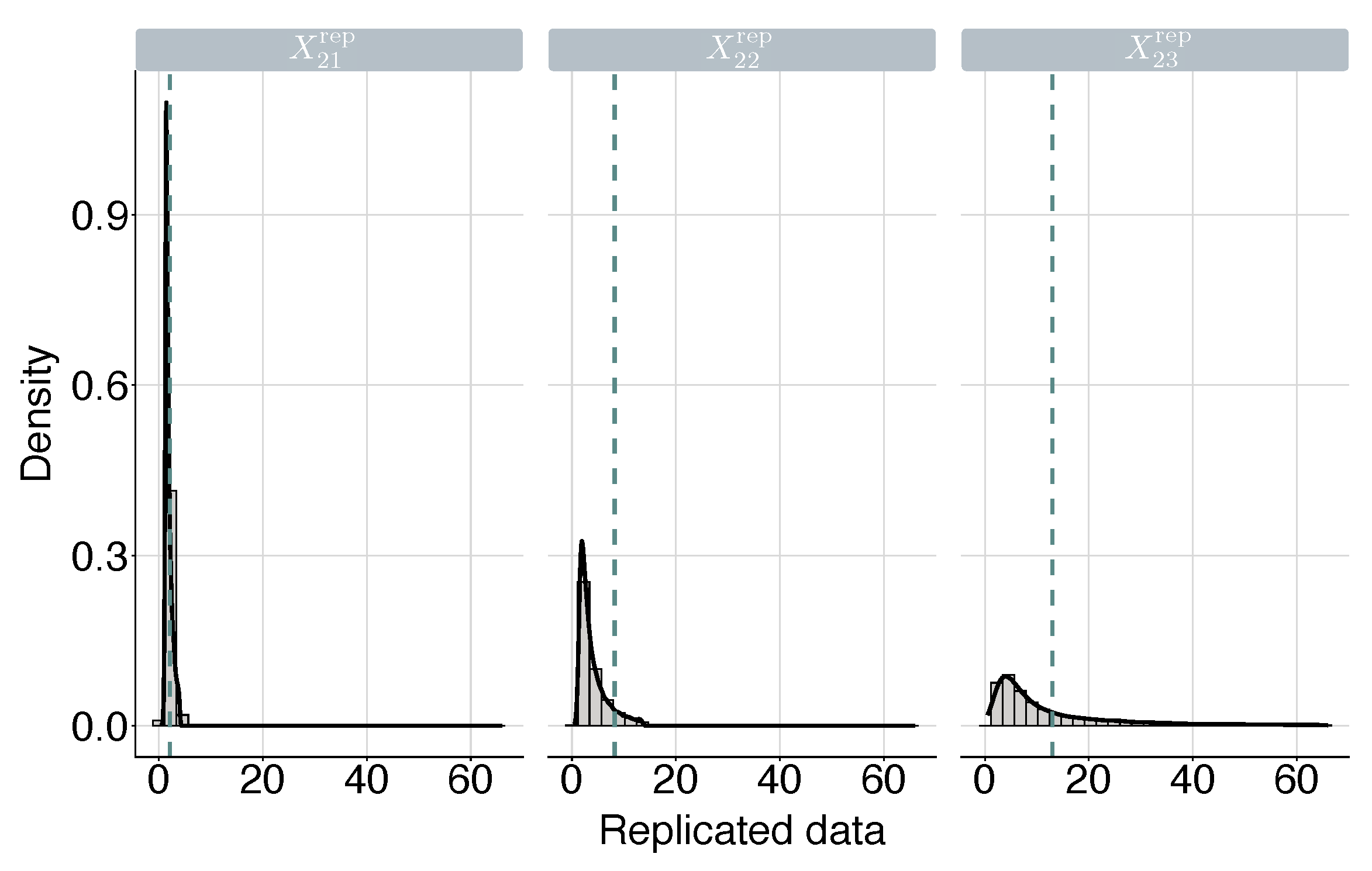
4.3. Posterior Predictive Checking

Posterior predictive checking (PPC) is a Bayesian model diagnostic technique that evaluates whether the model adequately fits the observed data. It involves generating the replicated data from the posterior predictive distribution and comparing them with the observed data. If the model is well fitting, the replicated data are similar to the observed data, indicating that the model appropriately describes the underlying structure of the observed data.

Let ${\mathit{X}}_i^{\mathrm{rep}}=\left\{X_{i1}^{\mathrm{rep}},\dots ,X_{ik}^{\mathrm{rep}}\right\}$ be the replicated data of the observed data ${\mathit{x}}_i=\left\{x_{i1},\dots ,x_{ik}\right\}$ for $i=1,\dots ,m$. Then, the Bayesian predictive density function of $X_{ij}^{\mathrm{rep}}$ under the prior (12) is given by

$$\begin{array}{cc}\hfill f_{X_{ij}^{\mathrm{rep}}}^{\ast }\left(x_{ij}^{\mathrm{rep}}\right)=& {\int }_{\theta }{\int }_{{\lambda }_1}{\int }_{{\lambda }_2}{f}_{X_{ij}^{\mathrm{rep}}}\left(x_{ij}^{\mathrm{rep}}|\mathit{\varphi }\right)\pi \left(\mathit{\varphi }|\mathit{x},\mathit{y}\right)\mathrm{d}{\lambda }_2\mathrm{d}{\lambda }_1\mathrm{d}\theta ,\hfill \\ \hfill & i=1,\dots ,m\mathrm{and}j=1,\dots ,k,\hfill \end{array}$$

where $f_{X_{ij}^{\mathrm{rep}}}\left(x_{ij}^{\mathrm{rep}}|\mathit{\varphi }\right)$ is the density function of $X_{ij}^{\mathrm{rep}}$ given $\mathit{\varphi }$. Likewise, let ${\mathit{Y}}^{\mathrm{rep}}=\left\{Y_1^{\mathrm{rep}},\dots ,Y_m^{\mathrm{rep}}\right\}$ be the replicated data of the observed data $\mathit{y}=\left\{y_1,\dots ,y_m\right\}$. The resulting Bayesian predictive density function of $Y_i^{\mathrm{rep}}$ under the prior (12) is given by

$$\begin{array}{cc}\hfill f_{Y_i^{\mathrm{rep}}}^{\ast }\left(y_i^{\mathrm{rep}}\right)=& {\int }_{\theta }{\int }_{{\lambda }_1}{\int }_{{\lambda }_2}{f}_{Y_i^{\mathrm{rep}}}\left(y_i^{\mathrm{rep}}|\mathit{\varphi }\right)\pi \left(\mathit{\varphi }|\mathit{x},\mathit{y}\right)\mathrm{d}{\lambda }_2\mathrm{d}{\lambda }_1\mathrm{d}\theta ,\hfill \\ \hfill & i=1,\dots ,m,\hfill \end{array}$$

where $f_{Y_i^{\mathrm{rep}}}\left(y_i^{\mathrm{rep}}|\mathit{\varphi }\right)$ is the density function of $Y_i^{\mathrm{rep}}$ given $\mathit{\varphi }$. To examine the appropriateness of the fitted model, we employ the posterior predictive p-value (PPP), which quantifies how similar the replicated data are to the observed data. Empirically, PPPs are computed as

$$\begin{array}{cc}\hfill & {\mathrm{PPP}}_{X_i}={\displaystyle \frac{1}{N^{\mathrm{rep}}}}\sum _{l=1}^{N^{\mathrm{rep}}}\mathbb{1}\left(\mathcal{T}\left({\mathit{x}}_i^{\mathrm{rep},l}\right)\ge \mathcal{T}\left({\mathit{x}}_i\right)\right),i=1,\dots ,m,\hfill \end{array}$$

and

$$\begin{array}{c}{\mathrm{PPP}}_Y={\displaystyle \frac{1}{N^{\mathrm{rep}}}}\sum _{l=1}^{N^{\mathrm{rep}}}\mathbb{1}\left(\mathcal{T}\left({\mathit{y}}^{\mathrm{rep},l}\right)\ge \mathcal{T}\left(\mathit{y}\right)\right),\hfill \end{array}$$

where $N^{\mathrm{rep}}$ is the number of the replicated data generated, and ${\mathit{X}}_i^{\mathrm{rep},l}$ and ${\mathit{Y}}^{\mathrm{rep},l}$ denote the lth replicated data of the observed data ${\mathit{x}}_i$ and $\mathit{y}$, respectively. According to Gelman et al. [16], PPP within the range of 0.05 to 0.95 is reasonably considered, supporting the appropriateness of the fitted model.

5. Application

This section assesses the performance of the proposed method via Monte Carlo simulations with 1000 simulated datasets and validates its practical applicability through a real-world case study using the software failure time data.

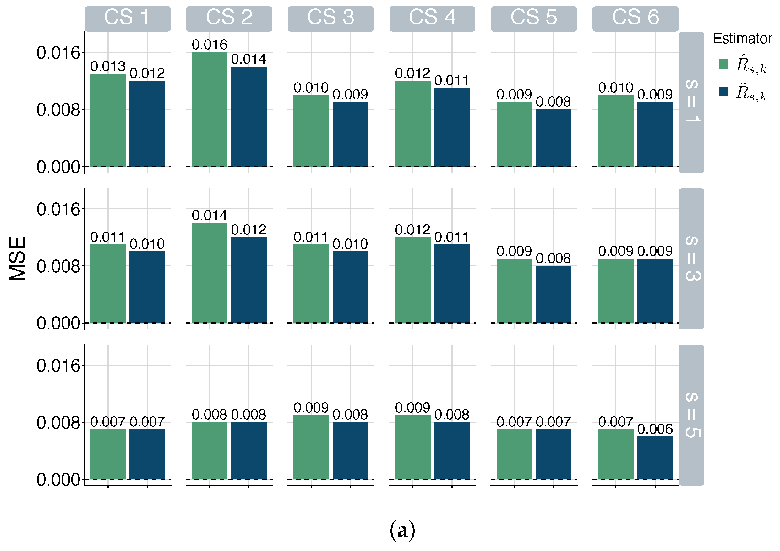
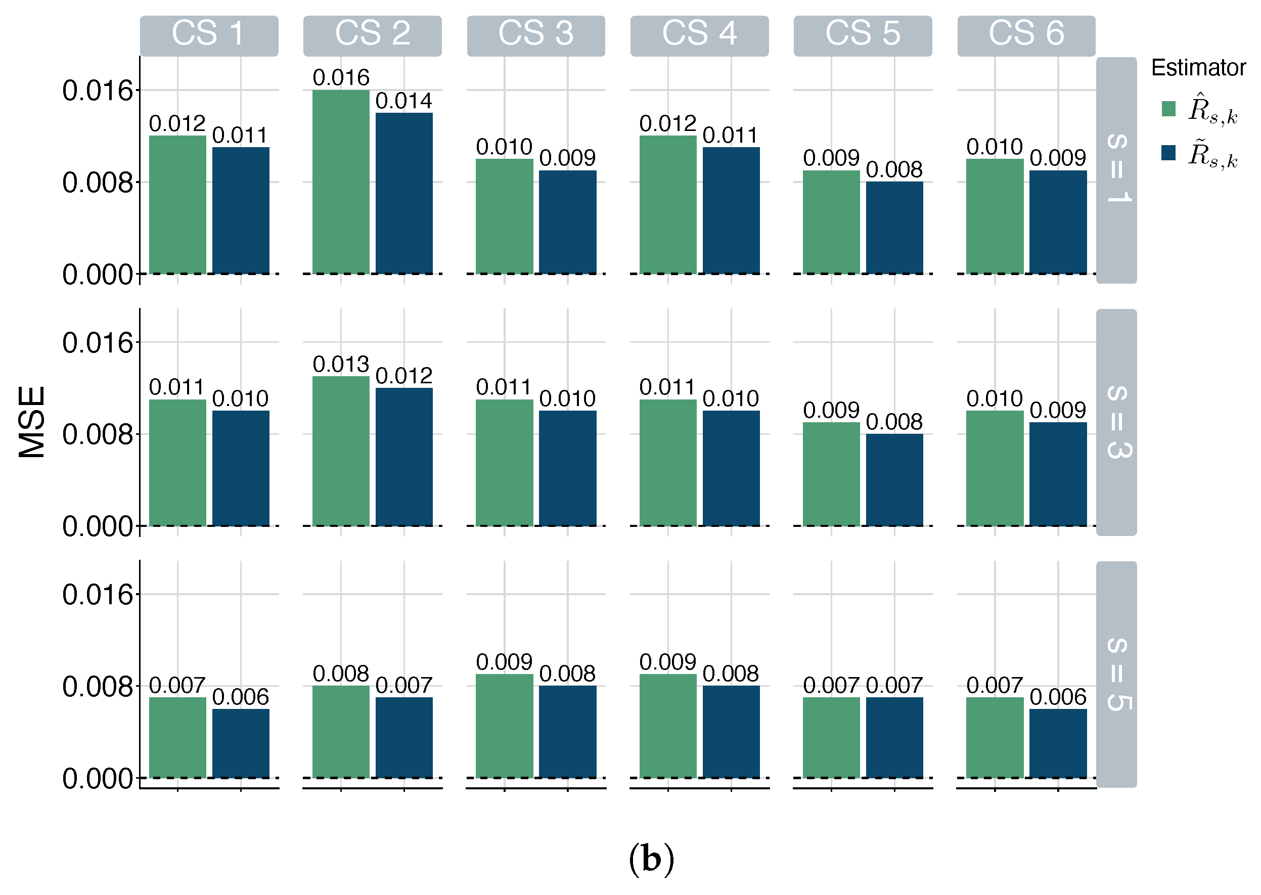
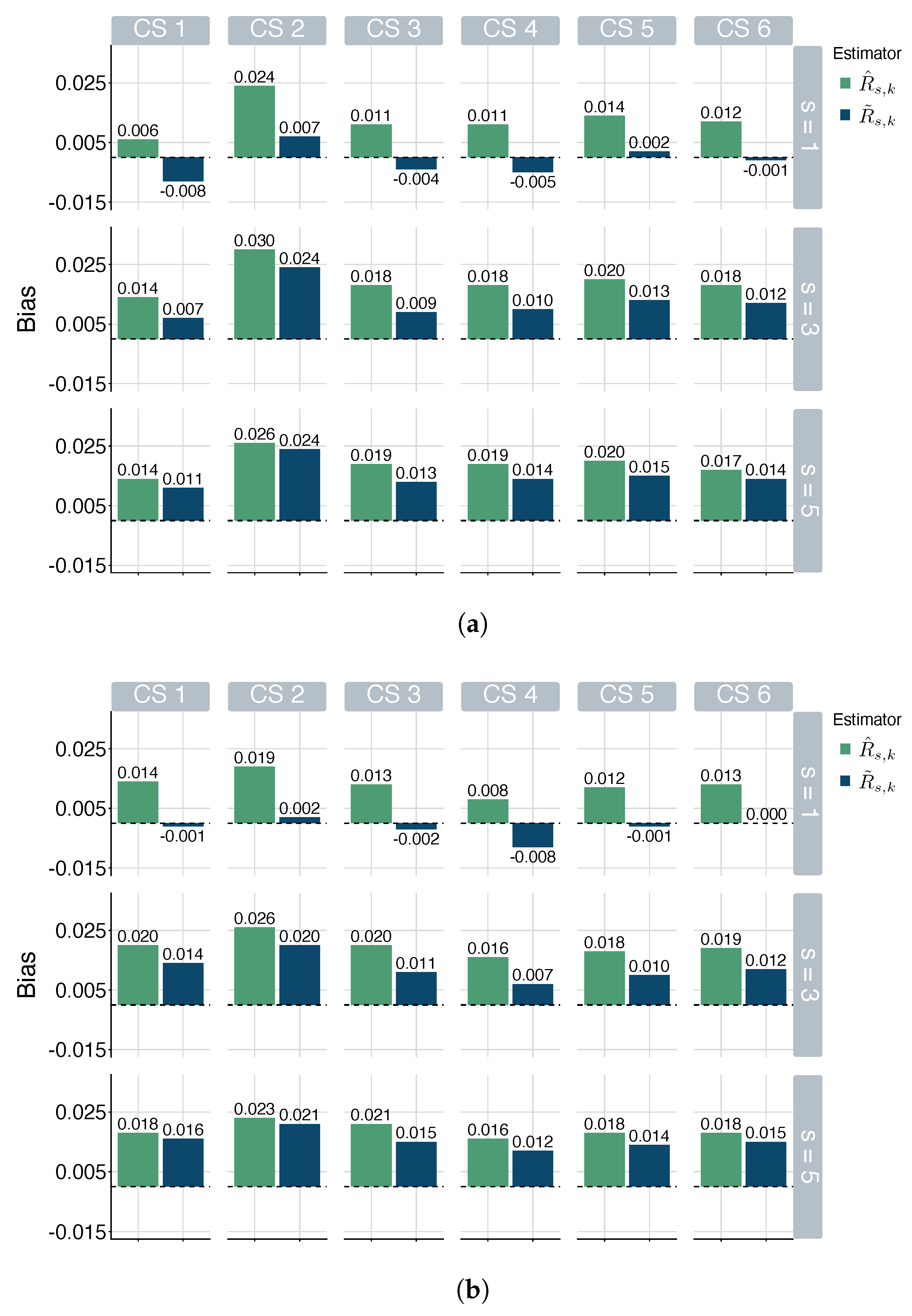
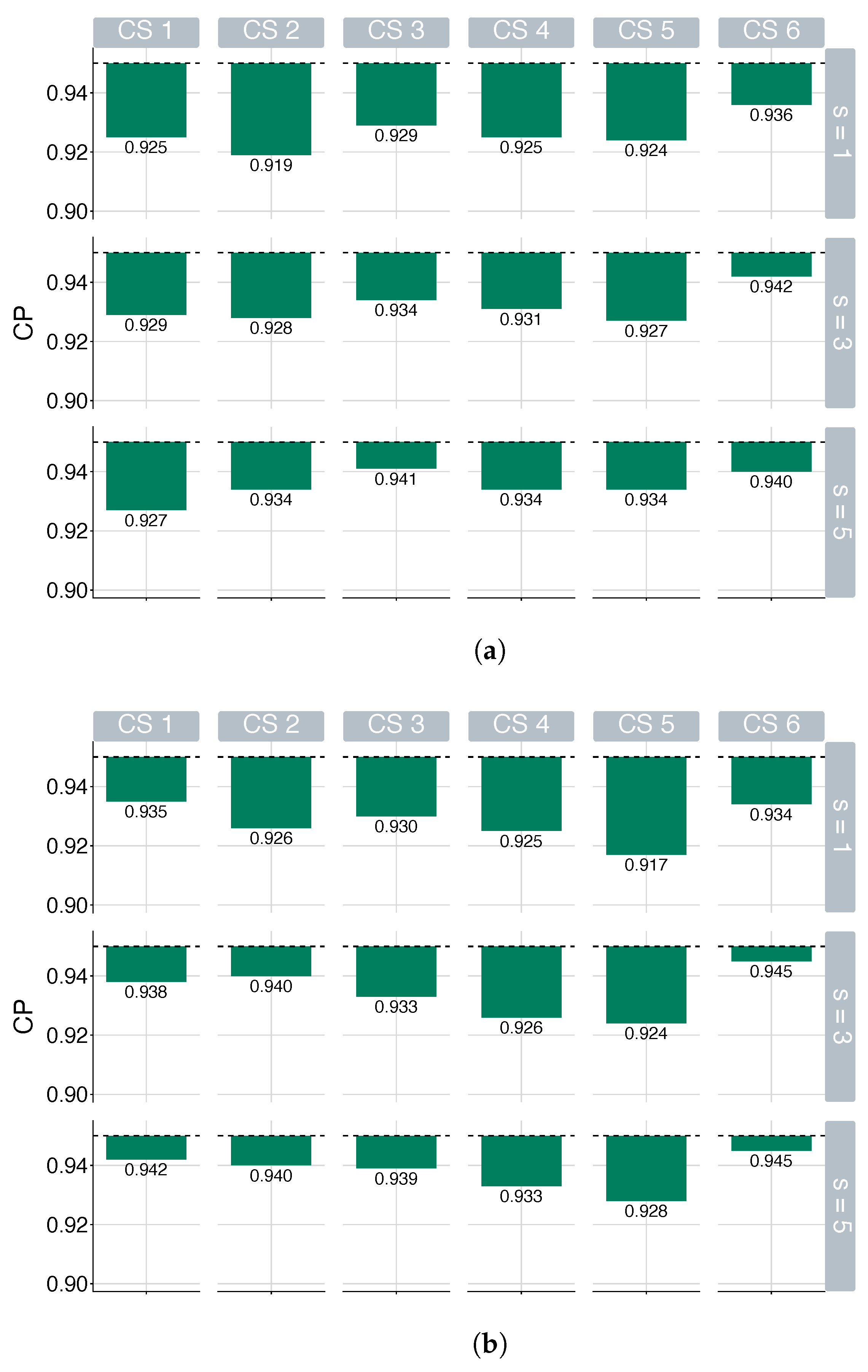
5.1. Simulation Study

This subsection provides a comprehensive assessment of the proposed Bayesian estimation method using various statistical metrics, focusing on the reliability (3) of the multicomponent stress–strength model based on the Pareto distribution with the CDF (2) under the APT-II CS. For the simulation study, different values of s, $s=1\left(2\right)5$, are considered to examine its influence on reliability. The true parameter values of the Pareto distribution are set to $\theta =1$, ${\lambda }_1=1.5$, and ${\lambda }_2=0.5$, and the time thresholds are assigned as $T_X=1.5$ and $T_Y=2.5$. Furthermore, to substantiate the effectiveness of the proposed method under small sample conditions, we employ the CSs detailed in

Table 1. CSs considered for the simulation study.

Pattern	CS	$n_X$	$n_Y$	k	m	${\mathcal{R}}^{\mathrm{STH}}=\left(R_1^{\mathrm{STH}},\dots ,R_k^{\mathrm{STH}}\right)$	${\mathcal{R}}^{\mathrm{STS}}=\left(R_1^{\mathrm{STS}},\dots ,R_m^{\mathrm{STS}}\right)$
Pattern 1	1	20	20	12	10	$(0\ast 3,1\ast 5,0\ast 3,3)$	$(0\ast 2,1\ast 4,0\ast 3,6)$
	2			10	8	$(0\ast 2,1\ast 4,0\ast 3,6)$	$(0\ast 1,1\ast 3,0\ast 3,9)$
	3	30	20	20	12	$(0\ast 7,1\ast 9,0\ast 3,1)$	$(0\ast 3,1\ast 5,0\ast 3,3)$
	4			16	10	$(0\ast 5,1\ast 7,0\ast 3,7)$	$(0\ast 2,1\ast 4,0\ast 3,6)$
	5	30	30	18	14	$(0\ast 6,1\ast 8,0\ast 3,4)$	$(0\ast 4,1\ast 6,0\ast 3,10)$
	6			14	12	$(0\ast 4,1\ast 6,0\ast 3,10)$	$(0\ast 3,1\ast 5,0\ast 3,13)$
Pattern 2	1	20	20	12	10	$(1\ast 3,0\ast 6,1\ast 2,3)$	$(1\ast 2,0\ast 5,1\ast 2,6)$
	2			10	8	$(1\ast 2,0\ast 5,1\ast 2,6)$	$(1\ast 1,0\ast 4,1\ast 2,9)$
	3	30	20	20	12	$(1\ast 7,0\ast 10,1\ast 3)$	$(1\ast 3,0\ast 6,1\ast 2,3)$
	4			16	10	$(1\ast 5,0\ast 8,1\ast 2,7)$	$(1\ast 2,0\ast 5,1\ast 2,6)$
	5	30	30	18	14	$(1\ast 6,0\ast 9,1\ast 2,4)$	$(1\ast 4,0\ast 7,1\ast 2,10)$
	6			14	12	$(1\ast 4,0\ast 7,1\ast 2,10)$	$(1\ast 3,0\ast 6,1\ast 2,13)$

${\mathcal{R}}^{\mathrm{STH}}$ and ${\mathcal{R}}^{\mathrm{STS}}$ denote the PT-II CSs for the strength and stress samples, respectively, and $0\ast 2$ indicates a zero vector of length 2.

, following the patterns outlined below.

$$\begin{array}{cc}\hfill \mathrm{Pattern} 1:& {\mathcal{R}}_1=\cdots ={\mathcal{R}}_{(j-6)/2}=0,{\mathcal{R}}_{(j-6)/2+1}=\cdots ={\mathcal{R}}_{j-4}=1,\hfill \\ \hfill & {\mathcal{R}}_{j-3}=\cdots ={\mathcal{R}}_{j-1}=0,{\mathcal{R}}_j=n-{\displaystyle \frac{3j}{2}}+1\hfill \\ \hfill \mathrm{Pattern} 2:& {\mathcal{R}}_1=\cdots ={\mathcal{R}}_{(j-6)/2}=1,{\mathcal{R}}_{(j-6)/2+1}=\cdots ={\mathcal{R}}_{j-3}=0,\hfill \\ \hfill & {\mathcal{R}}_{j-2}={\mathcal{R}}_{j-1}=1,{\mathcal{R}}_j=n-{\displaystyle \frac{3j}{2}}+1,\hfill \\ \hfill & \mathrm{where} j=\left\{\begin{array}{c}k, \mathrm{for} \mathrm{the} \mathrm{strength} \mathrm{sample},\hfill \\ m, \mathrm{for} \mathrm{the} \mathrm{stress} \mathrm{sample}.\hfill \end{array}\right.\hfill \end{array}$$

The APT-II censored sample for the strength variable in a single component system is generated using the algorithm of Ng et al. [6]. The explanation of the algorithm is detailed below, and the PT-II censored strength sample is denoted by $X_{i,1:k:n_X},\dots ,X_{i,k:k:n_X}$ to avoid confusion with the APT-II censored sample.

(1)

Generate an ordinary PT-II censored sample $X_{i,1:k:n_X},\dots ,X_{i,k:k:n_X}$ with the CS $\left({\mathcal{R}}_1^{\mathrm{STH}},\dots ,{\mathcal{R}}_k^{\mathrm{STH}}\right)$ from the algorithm of Balakrishnan and Sandhu [17] as follows:

(a)

Generate k independent realizations $W_1,\dots ,W_k$ from the standard uniform distribution.

(b)

Compute $V_j=W_j^{{\left(j+{\mathcal{R}}_k^{\mathrm{STH}}+\cdots +{\mathcal{R}}_{k-j+1}^{\mathrm{STH}}\right)}^{-1}}$ for $j=1,\dots ,k$.

(c)

Compute $U_j=1-V_k\cdots V_{k-j+1}$ for $j=1,\dots ,k$.

(d)

Compute $X_{i,j:k:n_X}=\theta /{(1-U_j)}^{1/{\lambda }_1}$ for $j=1,\dots ,k$, which is a PT-II censored sample for the strength variable from the Pareto distribution with the CDF (2) in a single component system.

(2)

Determine the value of $D_{i,1}$ satisfying $X_{i,D_{i,1}:k:n_X}<T_X<X_{i,D_{i,1}+1:k:n_X}$.

(3)

Generate the first $k-d_{i,1}-1$ order statistics from a truncated distribution $f_X\left(x\right)/\left[1-F_X\left(x_{i,d_{i,1}+1:k:n_X}\right)\right]$ with sample size $n_X-{\displaystyle \sum _{j=1}^{d_{i,1}}}\left(1+{\mathcal{R}}_j^{\mathrm{STH}}\right)-1$, where $f_X(·)$ denotes the PDF of the strength variable.

(4)

Substitute $X_{i,d_{i,1}+2:k:n_X},\dots ,X_{i,k:k:n_X}$ with the first $k-d_{i,1}-1$ order statistics obtained in (3).

• In a similar manner, multicomponent APT-II censored samples are generated by considering m-out-of-$n_Y$ systems coupled with k-out-of-$n_X$ components. The APT-II censored sample for the stress variable is also generated using the algorithm of Ng et al. [6].

To implement the NUTS algorithm for MCMC sampling in the proposed method, RStan [18] is utilized. The MCMC procedure consists of 10,000 iterations, of which the first 2000 are discarded as burn-in. Based on the remaining 8000 MCMC samples, the Bayes estimator (15) and HPD CrI are computed. The performance of the Bayes estimator (15) is evaluated by comparing it with the MLE (5) in terms of mean squared errors (MSEs) and biases. In addition, the validity of the HPD CrI under the prior (12) is examined through an analysis of coverage probabilities (CPs) and average lengths (ALs) at the 0.95 level. The results for the ACI (8) are not presented, as the true values of ${\lambda }_1$ and ${\lambda }_2$ under the CSs specified in Table 1 do not satisfy the constraints (9). Specifically, well-defined variances are ensured under ${\lambda }_1<0.46$ and ${\lambda }_2<0.4$. However, imposing such strict constraints on both parameters simultaneously is unrealistic in practical applications.

The simulation results are reported in Figure 1, Figure 2, Figure 3 and Figure 4, which provide the following key observations: First, across all scenarios, ${\tilde{R}}_{s,k}$ generally outperforms ${\widehat{R}}_{s,k}$ in terms of both MSE and bias, exhibiting overall smaller bias values. Second, for fixed CSs, the MSE values of both estimators generally decrease as s increases. Regarding bias, the case of $s=1$ tends to yield a smaller bias than the case of $s=5$ for fixed CSs. Third, the HPD CrI under the prior (12) achieves CPs close to $0.95$ across all scenarios, and its ALs generally decrease as s increases for fixed CSs. These patterns remain stable across both Pattern 1 and Pattern 2, indicating the consistency of the findings.

Taken together, the proposed method not only provides a less biased estimation of the multicomponent stress–strength reliability (3) but also ensures reliable uncertainty quantification, even in small-sample settings. In particular, the likelihood-based method struggles to construct the ACI due to constraints, whereas the proposed method remains stable and performs well across all scenarios. These findings demonstrate that the proposed method offers a competitive and effective alternative to the likelihood-based method for multicomponent stress–strength reliability analysis.

5.2. Software Failure Time Data

This subsection analyzes the data originally introduced by Musa [19] and later examined in detail by Kayal et al. [20]. These data contain the times of software failures recorded during the system test phase. Let $Y_1^{\mathrm{Total}}$ denote the 17th recorded failure time, and $X_{1j}^{\mathrm{Total}}$$(j=1,2,\cdots ,6)$ represent the failure times corresponding to observations indexed from 18 to 23. Similarly, $Y_2^{\mathrm{Total}}$ denotes the failure time of the 24th observation, and $X_{2j}^{\mathrm{Total}}$$(j=1,2,\cdots ,6)$ represent the failure times of the observations numbered 25 through 30. By continuing the data process up to the 51st failure time, we obtain the following data:

$$\begin{array}{c}\hfill {\mathit{X}}^{\mathrm{Total}}=\left(\begin{array}{cccccc}277& 596& 757& 437& 2230& 437\\ 405& 535& 277& 363& 522& 613\\ 1300& 821& 213& 1620& 1601& 298\\ 618& 2640& 5& 149& 1034& 2441\\ 565& 1119& 437& 927& 4462& 714\end{array}\right) \mathrm{and} {\mathit{Y}}^{\mathrm{Total}}=\left(\begin{array}{c}135\\ 340\\ 277\\ 874\\ 460\end{array}\right).\end{array}$$

For computational efficiency, the failure time data are rescaled by dividing all values by 100. Based on the scaled data, the following settings are adopted to obtain multicomponent APT-II censored samples:

$$\begin{array}{cc}\hfill & n_X=6,k=3,{\mathcal{R}}^{\mathrm{STH}}=(1,1,1),T_X=3.5,\hfill \\ \hfill & n_Y=5,m=3,{\mathcal{R}}^{\mathrm{STS}}=(0,1,1),T_Y=2.5.\hfill \end{array}$$

Under these settings, the APT-II CS is initially applied to ${\mathit{Y}}^{\mathrm{Total}}$. Then, rows in ${\mathit{X}}^{\mathrm{Total}}$ corresponding to the censored observations in ${\mathit{Y}}^{\mathrm{Total}}$ are removed. Subsequently, the APT-II CS is applied to the remaining rows of ${\mathit{X}}^{\mathrm{Total}}$. The resulting APT-II censored data for the strength and stress variables are given by

$$\begin{array}{c}\hfill {\mathit{X}}^{{\mathcal{R}}^{\ast }}=\left(\begin{array}{ccc}2.77& 4.37& 5.96\\ 2.13& 8.21& 13.00\\ 2.77& 4.05& 5.22\end{array}\right) \mathrm{and} {\mathit{Y}}^{{\mathcal{R}}^{\ast }}=\left(\begin{array}{c}1.35\\ 2.77\\ 3.40\end{array}\right),\end{array}$$

respectively.

For the proposed method, a total of 15,000 MCMC samples for $\theta$ are generated, with the first 3000 discarded as part of the burn-in phase. When considering a 1-out-of-3 system, the estimation results are reported in

Table 2. Estimation results of $\mathit{\varphi }$ and $R_{1,3}\left(\mathit{\lambda }\right)$ for the software failure time data.

Likelihood-Based Approach				Proposed Bayesian Approach
$\widehat{\theta }$	${\widehat{\lambda }}_1$	${\widehat{\lambda }}_2$	${\widehat{R}}_{1,3}$	$\tilde{\theta }$	${\tilde{\lambda }}_1$	${\tilde{\lambda }}_2$	${\tilde{R}}_{1,3}$	HPD CrI
1.350	0.388	0.860	0.915	1.235	0.362	0.763	0.852	(0.563, 0.999)

. The ACI (8) is not computed because the estimate of ${\widehat{\lambda }}_2$ does not satisfy the constraint (9) under the considered CS.

Assessing the convergence of the MCMC chains for $\theta$ is crucial for ensuring the validity of Bayesian inference. To this end, a suite of diagnostic tools is employed, including the effective sample size and a trace plot. First, the effective sample size of $3808.477$ is sufficiently large, suggesting low autocorrelation and ensuring a reliable effective sample size. The trace plot is depicted in Figure 5, which exhibits desirable characteristics, such as stationarity and the absence of discernible trends or periodicity. Taken together, these diagnostics provide strong evidence that the MCMC chain for $\theta$ has converged adequately.

Additionally, Figure 6 presents the histograms and estimated kernel densities of MCMC samples for $\theta$, ${\lambda }_1$, and ${\lambda }_2$, showing that the density for $\theta$ has a long left tail, whereas the densities for ${\lambda }_1$ and ${\lambda }_2$ exhibit pronounced right skewness. Moreover, Figure 7 displays the histogram and estimated kernel density of MCMC samples for $R_{1,3}\left(\mathit{\lambda }\right)$, our primary focus, which exhibits a distinct left-skewed pattern.

To examine whether the fitted model adequately captures the characteristics of the obtained APT-II censored data, PPC is conducted. In this process, 12,000 replicated data are generated, and PPPs are computed based on these replicated data using the mean and standard deviation (SD) as test statistics. The results are reported in

Table 3. PPPs computed using the replicated data and the obtained APT-II censored data.

	${\mathrm{PPP}}_{X_1}$	${\mathrm{PPP}}_{X_2}$	${\mathrm{PPP}}_{X_3}$	${\mathrm{PPP}}_Y$
Mean	0.596	0.385	0.633	0.545
SD	0.722	0.428	0.793	0.511

, which indicates that the fitted model adequately explains the obtained APT-II censored data. For further examination, the estimated kernel densities of the replicated data are analyzed.

Table 4. Skewness for the densities of the replicated data.

$X_1^{\mathrm{rep}}$			$X_2^{\mathrm{rep}}$			$X_3^{\mathrm{rep}}$			$Y^{\mathrm{rep}}$
$X_{11}^{\mathrm{rep}}$	$X_{12}^{\mathrm{rep}}$	$X_{13}^{\mathrm{rep}}$	$X_{21}^{\mathrm{rep}}$	$X_{22}^{\mathrm{rep}}$	$X_{23}^{\mathrm{rep}}$	$X_{31}^{\mathrm{rep}}$	$X_{32}^{\mathrm{rep}}$	$X_{33}^{\mathrm{rep}}$	$Y_1^{\mathrm{rep}}$	$Y_2^{\mathrm{rep}}$	$Y_3^{\mathrm{rep}}$
32.38	104.30	109.49	107.12	102.49	109.48	107.48	77.73	109.52	109.52	78.65	109.51

reports the skewness values of the densities based on 12,000 replicated data, exhibiting the presence of extreme skewness. To improve visualization, excessively large values are truncated, and the resulting histograms and estimated kernel densities are displayed in Figure 8, Figure 9, Figure 10 and Figure 11. These plots indicate that the observations are generally located in regions of high Bayesian predictive density. These findings reveal that the fitted model is capable of generating the replicated data that closely resemble the obtained APT-II censored data, effectively capturing its underlying characteristics.

6. Conclusions

This study proposed an objective Bayesian framework for estimating the reliability of the multicomponent stress–strength model based on the Pareto distribution under the APT-II CS. By incorporating a reference prior with partial information, the proposed Bayesian framework effectively addresses the limitations of the classical likelihood-based method, particularly the issue of the AVCM not being well defined, thereby enhancing the stability and accuracy of inference. This framework also serves as a practical alternative to the bootstrap method, which is commonly used for uncertainty quantification but exhibits structural limitations when applied to the Pareto distribution. Since the MLE of $\theta$ is determined by the first-order statistic, it is always greater than $\theta$ due to the support $(\theta ,\infty )$, and the resulting estimation error becomes more severe in small samples, leading to inaccurate inference. These issues make clear the advantages of the proposed framework, particularly in small sample scenarios.

In real-world applications involving censored data, collecting large samples is often infeasible due to the inherent constraints in time, cost, and experimental conditions. For this reason, statistical inference under CSs is frequently conducted under small sample conditions. To reflect this practical limitation, we also considered small sample scenarios in our simulation studies. Under these settings, the Bayes estimator demonstrated its superiority over the MLE, exhibiting lower MSE and bias values across various censoring scenarios. Moreover, the HPD CrI consistently achieved CPs close to the considered nominal level. These results reveal that the proposed method offers a stable and reliable reliability estimation, even in cases where sample sizes are insufficient, unlike the likelihood-based method, which struggles to construct the ACI due to constraints. The practical feasibility of the proposed approach was validated through real-world data analysis on software failure times, underscoring its applicability in reliability assessment for complex engineering and industrial systems.

Future research can extend the proposed framework to other distributions or incorporate hierarchical modeling techniques to better capture system-level dependencies. Moreover, in practical scenarios where strength and stress variables may be correlated, extended models incorporating correlation structures, such as those based on copula functions, can be explored.

References

1. Bhattacharyya, G.K.; Johnson, R.A. Estimation of reliability in a multicomponent stress-strength model. J. Am. Stat. Assoc. 1974, 69, 966–970. [Google Scholar] [CrossRef]
2. Wang, L.; Wu, K.; Tripathi, Y.M.; Lodhi, C. Reliability analysis of multicomponent stress-strength reliability from a bathtub-shaped distribution. J. Appl. Stat. 2022, 49, 122–142. [Google Scholar] [CrossRef] [PubMed]
3. Lio, Y.; Tsai, T.R.; Wang, L.; Cecilio Tejada, I.P. Inferences of the multicomponent stress-strength reliability for Burr XII distributions. Mathematics 2022, 10, 2478. [Google Scholar] [CrossRef]
4. Jha, M.K.; Dey, S.; Alotaibi, R.; Alomani, G.; Tripathi, Y.M. Multicomponent stress-strength reliability estimation based on unit generalized exponential distribution. Ain Shams Eng. J. 2022, 13, 101627. [Google Scholar] [CrossRef]
5. Jana, N.; Bera, S. Interval estimation of multicomponent stress-strength reliability based on inverse Weibull distribution. Math. Comput. Simul. 2022, 191, 95–119. [Google Scholar] [CrossRef]
6. Ng, H.K.T.; Kundu, D.; Chan, P.S. Statistical analysis of exponential lifetimes under an adaptive Type-II progressive censoring scheme. Nav. Res. Logist. 2009, 56, 687–698. [Google Scholar] [CrossRef]
7. Chen, S.; Gui, W. Statistical analysis of a lifetime distribution with a bathtub-shaped failure rate function under adaptive progressive Type-II censoring. Mathematics 2020, 8, 670. [Google Scholar] [CrossRef]
8. Ateya, S.F.; Amein, M.M.; Mohammed, H.S. Prediction under an adaptive progressive Type-II censoring scheme for Burr Type-XII distribution. Commun. Stat.-Theory Methods 2022, 51, 4029–4041. [Google Scholar] [CrossRef]
9. Dutta, S.; Dey, S.; Kayal, S. Bayesian survival analysis of logistic exponential distribution for adaptive progressive Type-II censored data. Comput. Stat. 2024, 39, 2109–2155. [Google Scholar] [CrossRef]
10. Azhad, Q.J.; Arshad, M.; Khandelwal, N. Statistical inference of reliability in multicomponent stress strength model for Pareto distribution based on upper record values. Int. J. Model. Simul. 2022, 42, 319–334. [Google Scholar] [CrossRef]
11. Jeffreys, H. An invariant form for the prior probability in estimation problems. Proc. R. Soc. Lond. Ser. A Math. Phys. Sci. 1946, 186, 453–461. [Google Scholar]
12. Sun, D.; Berger, J.O. Reference priors with partial information. Biometrika 1998, 85, 55–71. [Google Scholar] [CrossRef]
13. Hoffman, M.D.; Gelman, A. The No-U-Turn sampler: Adaptively setting path lengths in Hamiltonian Monte Carlo. J. Mach. Learn. Res. 2014, 15, 1593–1623. [Google Scholar]
14. Duane, S.; Kennedy, A.D.; Pendleton, B.J.; Roweth, D. Hybrid Monte Carlo. Phys. Lett. B 1987, 195, 216–222. [Google Scholar] [CrossRef]
15. Chen, M.H.; Shao, Q.M. Monte Carlo estimation of Bayesian credible and HPD intervals. J. Comput. Graph. Stat. 1999, 8, 69–92. [Google Scholar] [CrossRef]
16. Gelman, A.; Carlin, J.B.; Stern, H.S.; Dunson, D.B.; Vehtari, A.; Rubin, D.B. Bayesian Data Analysis, 3rd ed.; Chapman and Hall/CRC: Boca Raton, FL, USA, 2013. [Google Scholar]
17. Balakrishnan, N.; Sandhu, R.A. A simple simulational algorithm for generating progressive Type-II censored samples. Am. Stat. 1995, 49, 229–230. [Google Scholar] [CrossRef]
18. Stan Development Team. RStan: The R Interface to Stan, R Package Version 2.32.3. 2023. Available online: https://mc-stan.org/ (accessed on 15 December 2022).
19. Musa, J.D. Software Reliability Data; Technical Report; Data and Analysis Center for Software, Rome Air Development Center: Rome, NY, USA, 1979. [Google Scholar]
20. Kayal, T.; Tripathi, Y.M.; Dey, S.; Wu, S.J. On estimating the reliability in a multicomponent stress-strength model based on Chen distribution. Commun. Stat.-Theory Methods 2020, 49, 2429–2447. [Google Scholar] [CrossRef]
Figure 1. MSEs of estimators for R s , k ( λ ) in (a) Pattern 1 and (b) Pattern 2.
Mathematics 13 01379 g001aMathematics 13 01379 g001b
Figure 2. Biases of estimators for R s , k ( λ ) in (a) Pattern 1 and (b) Pattern 2.
Mathematics 13 01379 g002
Figure 3. CPs of 95% HPD CrIs for R s , k ( λ ) in (a) Pattern 1 and (b) Pattern 2.
Mathematics 13 01379 g003
Figure 4. ALs of 95% HPD CrIs for R s , k ( λ ) in (a) Pattern 1 and (b) Pattern 2.
Mathematics 13 01379 g004aMathematics 13 01379 g004b
Figure 5. Trace plot for θ .
Mathematics 13 01379 g005
Figure 6. Histograms and estimated kernel densities of MCMC samples for (a) θ , (b) λ 1 , and (c) λ 2 (Solid line: mean, Dashed line: HPD CrI).
Mathematics 13 01379 g006aMathematics 13 01379 g006b
Figure 7. Histogram and estimated kernel density of MCMC samples for R 1 , 3 ( λ ) (Solid line: mean, Dashed line: HPD CrI).
Mathematics 13 01379 g007
Figure 8. Histograms and estimated kernel densities of the replicated data for x 1 (Dash line: Observation).
Mathematics 13 01379 g008
Figure 9. Histograms and estimated kernel densities of the replicated data for x 2 (Dash line: Observation).
Mathematics 13 01379 g009
Figure 10. Histograms and estimated kernel densities of the replicated data for x 3 (Dash line: Observation).
Mathematics 13 01379 g010
Figure 11. Histograms and estimated kernel densities of the replicated data for y (Dash line: Observation).
Mathematics 13 01379 g011