New Strategies Based on Hierarchical Matrices for Matrix Polynomial Evaluation in Exascale Computing Era

Abstract

Advancements in computing platform deployment have acted as both push and pull elements for the advancement of engineering design and scientific knowledge. Historically, improvements in computing platforms were mostly dependent on simultaneous developments in hardware, software, architecture, and algorithms (a process known as co-design), which raised the performance of computational models. But, there are many obstacles to using the Exascale Computing Era sophisticated computing platforms effectively. These include but are not limited to massive parallelism, effective exploitation, and high complexity in programming, such as heterogeneous computing facilities. So, now is the time to create new algorithms that are more resilient, energy-aware, and able to address the demands of increasing data locality and achieve much higher concurrency through high levels of scalability and granularity. In this context, some methods, such as those based on hierarchical matrices (HMs), have been declared among the most promising in the use of new computing resources precisely because of their strongly hierarchical nature. This work aims to start to assess the advantages, and limits, of the use of HMs in operations such as the evaluation of matrix polynomials, which are crucial, for example, in a Graph Convolutional Deep Neural Network (GC-DNN) context. A case study from the GCNN context provides some insights into the effectiveness, in terms of accuracy, of the employment of HMs.

1. Introduction

Matrix polynomials’ role can be considered relevant in many application areas. For example, many methods for computing matrix functions $f\left(\mathit{A}\right)$, where f is a scalar function and $\mathit{A}\in {\Re }^{n\times n}$ and $f\left(\mathit{A}\right)$ represent a matrix of the same dimensions as $\mathit{A}$, require the evaluation of a matrix polynomial. Indeed, under some assumptions about the eigenvalues of matrix $\mathit{A}$, a matrix’s function $f\left(\mathit{A}\right)$ can be expressed by the following Taylor series (see Theorem 4.7 in [1]):

$$f\left(\mathit{A}\right)=\sum _{k=0}^{\infty }{a}_k{\left(\mathit{A}-\alpha \mathit{I}\right)}^k.$$

(1)

and hence approximated by a matrix polynomial in the form (see Theorem 4.8 in [1])

$$f\left(\mathit{A}\right)\approx \sum _{k=0}^K{a}_k{\left(\mathit{A}-\alpha \mathit{I}\right)}^k.$$

(2)

where $\mathit{I}$ is the identity matrix and where $a_k={\displaystyle \frac{f^{\left(k\right)}\left(\alpha \right)}{k!}}$. Many applications can be re-formulated using matrix functions of the type $f\left(\mathit{A}\right)$ and then approximated by a matrix polynomial such as (2). As examples, we can list the following ones:

• Differential equations offer a wealth of problems based on $f\left(\mathit{A}\right)$. Indeed, many semi-discretized Partial Differential Equations (PDEs) (for example, see application related to the computational simulation of Power Systems [2]) can be (re)-formulated based on the following expression:

  $${\displaystyle \frac{\partial y}{\partial t}}=\mathit{A}y+f\left(t,y\right),t\in \left[0,T\right],y\left(0\right)=c,y\in {\Re }^n,\mathit{A}\in {\Re }^{n\times n}.$$

  (3)

  where $f\left(t,y\right)$ contains the nonlinear terms and $\mathit{A}$ is a spatially discretized linear operator [1]. A large class of techniques known as exponential integrators use an explicit methodology to numerically integrate the remaining portion of the solution while treating the linear term exactly for (3). The characteristic of exponential integrators [3] is that they employ the exponential function of the differential equation’s Jacobian or an approximation of it. Since the late 1990s, they have garnered increased attention, primarily because of developments in numerical linear algebra that enabled the effective use of the methods [1].
  The Exponential Time Differencing (ETD) Euler method is a basic illustration of an exponential integrator. EDT enables computing an approximation $y_{n+1}$ in one of the N instants $t_{n+1},n=0,\dots ,N-1$ into which the interval $\left[0,T\right]$ is subdivided of the solution y of (3) by means of the following iterative formula:

  $$y_{n+1}=y_n{\psi }_0\left(h\mathit{A}\right)+h{\psi }_1\left(h\mathit{A}\right)f\left(t_n,y_n\right),$$

  (4)

  where $h={\displaystyle \frac{t_{n+1}-t_n}{N}}$ and where the functions ${\psi }_0\left(z\right)$ and ${\psi }_1\left(z\right)$ are defined as follows

  $$\begin{array}{ccc}\hfill {\psi }_0\left(z\right)& =& e^z,\hfill \end{array}$$

  (5)

  $$\begin{array}{ccc}\hfill {\psi }_1\left(z\right)& =& {\displaystyle \frac{e^z-1}{z}}.\hfill \end{array}$$

  (6)
  The evaluation of the matrix functions ${\psi }_0\left(h\mathit{A}\right)$ and ${\psi }_1\left(h\mathit{A}\right)$, required by the iterative formula (4), can then be approximated by the evaluation of a matrix polynomial of kind (2).
• In Markov models, which are utilized in many different fields (from sociology to statistics and finance), a matrix function related to matrix exponential $f\left(A\right)=e^{\mathit{A}}$ is crucial. Indeed, consider a time-homogeneous continuous-time Markov process in which individuals move among n states. The entry $\left(i,j\right)$ of the process’s transition probability matrix $\mathit{P}\left(t\right)\in {\Re }^{n\times n}$ represents the likelihood that an individual who begins in state i at time 0 will be in state j at time t (where $i,j=1,\dots ,n$). The transition intensity matrix $\mathit{Q}\in {\Re }^{n\times n}$ is associated with the process and is connected to $\mathit{P}\left(t\right)$ by

  $$\mathit{P}\left(t\right)=e^{\mathit{Q}t}.$$

  (7)
  Suppose a given transition matrix $\mathit{P}\left(1\right)$ has a generator $\mathit{Q}=log\left(\mathit{P}\left(1\right)\right)$; then, $\mathit{Q}$ can be used to construct $\mathit{P}\left(t\right)$ at other times through Equation (7). The evaluation of the matrix exponential, required by Equation (7), can then be approximated by the evaluation of a matrix polynomial of kind (2).

A more exhaustive example list of matrix functions that could benefit the polynomial approximations can be found in Higham [1].

In addition to the examples of matrix polynomial use mentioned above, we call attention to another example of an application using matrix polynomial evaluation that is related to the polynomials of the Graph Laplacian defined in the context of Graph Convolutional Deep Neural Networks [4,5] (see Section 4 for details).

Progress in the deployment of computing platforms has constituted both pull and push factors for the advancement of scientific knowledge and engineering design [6,7,8,9,10,11,12,13].

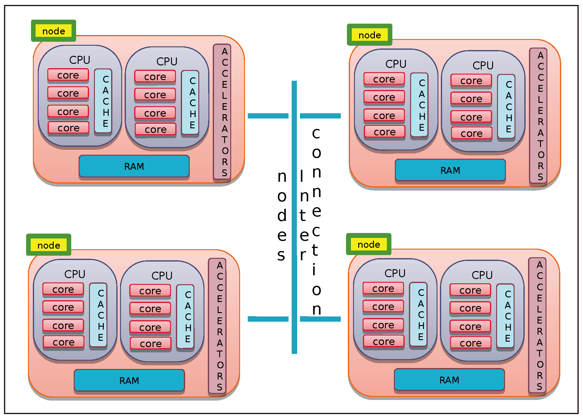
Historically, the high-performance computing (HPC) systems era started in the 1980s, when vector supercomputing dominated high-performance computing. Today, HPC systems are clusters composed of hundreds of nodes and millions of processors/cores where computational accelerators enrich each node in the form of coprocessors, such as General Purpose Graphical Processing Units (GP-GPUs), which are based on high-speed, low-latency interconnects (such as Infiniband) (see Figure 1 for a representation of modern HPC systems) [14].

The results of the popular high-performance LINPACK (HPL) benchmark [15], which is used to create the top 500 ranking of the fastest computers in the world [16], outline the exponential growth in advanced computing capabilities. A list like this demonstrates that the exascale (${10}^{18}$ operations per second) Era is the current state of affairs in the long performance improvement journey that has lasted over fifty years. In fact, the US Oak Ridge National Laboratory’s Frontier supercomputer broke the glass ceiling of the exascale barrier in the second half of 2022 [17]. Historically, improvements in computing platforms were mostly dependent on simultaneous developments in hardware, software, architecture, and algorithms (a process known as co-design), which raised the performance of computational models. But, there are many obstacles to using the Exascale Computing Era sophisticated computing platforms effectively. These include but are not limited to massive parallelism effective exploitation and high complexity in programming such heterogeneous computing facilities.

Research challenges in creating advanced computing systems for exascale objectives were identified by a number of studies [14,18,19].

From the perspective of a computational scientist, special relevance is assigned to the difficulties concerning new mathematical models and algorithms that can guarantee high degrees of scalability [20] and granularity [21], providing answers to the demand of increasing data locality and achieving much higher levels of concurrency. Thus, the time has come to create new algorithms that are more resilient, energy-conscious, and have fewer requirements for synchronization and communication.

To the best of our knowledge, the most recent analysis of the algorithms for polynomial evaluation for modern high-performance computing architectures can be found in [22]. The aim of that article was to evaluate the existing methods of polynomial evaluation on superscalar architecture, applying those methods to the computation of elementary functions such as $e^x$. The long story of parallel algorithms for polynomial evaluation starts with the work of Munro et al. [23], who first investigated parallel algorithms able to overcome the sequential nature of Horner’s algorithm [1]. Parallel polynomial evaluation was been the subject of much research over the past 50 years, such as described also by the survey contained in Ewart et al. [22], demonstrating the high level of interest in these algorithms.

In consideration that

… in pursuit of synchronization reduction, “additive operator” versions of sequentially “multiplicative operator” algorithms are often available … [24],

such work intends to explore new paths for matrix polynomial evaluation that are more suitable for exascale computing systems where synchronization points could be very demanding and where the heterogeneity and the hierarchical architecture of such systems suggest more appropriate algorithms for operations involving matrices.

Some methods for polynomial evaluations, such as the well-known Horner Method, suffer from a sequential nature and a high number of synchronization points or a low degree of parallelism. Furthermore, when matrix polynomials are based on sparse matrices, all the operations involving such matrices require constantly moving the sparse matrix entries from the main memory into the CPU, without register or cache reuse. Therefore, methods that demand less memory bandwidth need to be researched. To this extent, there are promising linear techniques, such as coefficient-matrix-free representations, that avoid sparse matrices, or Hierarchical matrices [25].

In the context just described, this paper aims to

• introduce some definitions and algorithms related to the concept of a hierarchical matrix;
• introduce an algorithm for matrix polynomial evaluation that has a good degree of parallelism;
• describe how such an algorithm can be combined with a hierarchical representation of a sparse matrix;
• highlight the benefits and limitations of using hierarchical matrices in the evaluation of matrix polynomials based on some case studies [4,5] (see Section 4 for details). The considered case studies are related to the matrix polynomials used in the context of Graph Convolutional Deep Neural Networks that in recent years have gained great importance in many areas, such as medicine, image analysis, and speech recognition, to generate data-driven models;
• provide some preliminary indications about the parallelization of the proposed algorithms.

The paper is structured as follows: in Section 2, the hierarchical matrices (HMs) are introduced and some algorithms of interest from basic matrix algebra that use HM formulations are described; Section 3 describes a strategy for the matrix polynomial evaluation based on the use of HMs that should be more suitable for exascale computing systems due to a reduced number of synchronization points and the hierarchical structure of HM-based operations; in Section 4, some results related to the use of the algorithms introduced in Section 2 and Section 3 are described to assess some advantages, and limits, of the use of HMs in a case study from the GCNN context. The study is summarized in Section 5, which also provides some information about our future work.

2. Fast Multipole Methods and Hierarchical Matrices

Fast Multipole Methods (FMMs), created by Rokhlin Jr. and Greengard [26], were named among the top 10 algorithms of the 20th century. They are first described in the context of particle simulations, where they reduce the computational cost, for each pairwise interaction in a system of N particles, from $O\left(N^2\right)$ to $O\left(N\right)$ or to $O\left(Nlog\left(N\right)\right)$ operations. In such a context, if ${\left\{{\mathit{x}}_i\right\}}_{i=1,\dots ,N}$ denote the locations of a set of N electrical charges and if ${\left\{q_i\right\}}_{i=1,\dots ,N}$ denote their source strengths, the aim of a particle simulation is to evaluate the potentials

$$u_i=\sum _{j=1}^{N}g\left({\mathit{x}}_i,{\mathit{x}}_j\right)q_j,i=1,\dots ,N$$

(8)

where $g\left({\mathit{x}}_i,{\mathit{x}}_j\right)$ is the interaction potential of electrostatics. The computation of all the values of vector $\mathit{u}={\left[u_i\right]}_{i=1,\dots ,N}^T$ can then be expressed as the following matrix–vector operation

$$\mathit{u}=\mathit{A}\mathit{q},$$

(9)

where the vector $\mathit{q}$ and the matrix $\mathit{A}$ are, respectively, defined as [27]

$$\mathit{q}={\left[q_i\right]}_{i=1,\dots ,N}^T\mathrm{and}\mathit{A}={\left[g\left({\mathit{x}}_i,{\mathit{x}}_j\right)\right]}_{i,j=1,\dots ,N}.$$

Considering that the kernel $g\left(\mathit{x},\mathit{y}\right)$ is smooth when $\mathit{x}$ and $\mathit{y}$ are not close, then, if I and J are two index subsets of $\left\{1,\dots ,N\right\}$ that represent two subsets of ${\left\{{\mathit{x}}_i\right\}}_{i\in I}$ and ${\left\{{\mathit{x}}_j\right\}}_{j\in J}$ of distant points, the sub-matrix ${\mathit{A}}_{IJ}={\left[g\left({\mathit{x}}_i,{\mathit{x}}_j\right)\right]}_{i\in I,j\in J}$ admits an approximate rank-P factorization of the kind

$${\mathit{A}}_{IJ}\approx \mathit{B}{\mathit{C}}^T,$$

(10)

where $\mathit{B},\mathit{C}$ have, respectively, $\left|I\right|\times P$ and $\left|J\right|\times P$ dimensions [27]. Then, every matrix–vector product involving the sub-matrix ${\mathit{A}}_{IJ}$ can be executed by just $O\left(P(M+N)\right)$ operations. In problem (9), no one relation like (10) can hold for all combinations of target and source points. The domain can then be considered cut into pieces, and approximations such as (10) can be used to evaluate interactions between distant pieces, and direct evaluation used only for points that are close. Equivalently, one could say that the matrix–vector product (9) can be computed by exploiting rank deficiencies in off-diagonal blocks of $\mathit{A}$ [27].

Then, throughout its history, FMM laid the groundwork for more practical uses, like the quick multiplication of vectors using completely populated special matrices [27,28,29]. In linear algebra, FMM is known as fast multiplication by $\mathcal{H}$-matrices, which is a combination of the Panel Clustering Method and the mosaic skeleton matrix approaches [13,30,31,32,33].

Paraphrasing Yokota et al. [34], “$\mathcal{H}$-matrices based one, appears to be an ideal algorithm for hybrid hierarchical distributed-shared memory architectures targeting billion-thread concurrency, which is the dominant design for contemporary extreme computing resources”.

The use of $\mathcal{H}$-matrices reduces the $O\left(m^2\right)$ asymptotic computational complexity $C_{Comp}\left(m\right)$ of a matrix–vector product $\mathit{A}\mathit{b}$, where $\mathit{A}\in {\Re }^{m\times m}$ and $\mathit{b}\in {\Re }^m$, to an $O\left((mlog\left(m\right)\right)$ or $O\left(m\right)$ one through a hierarchy of tree-based operations by distinguishing between near interactions that must be treated directly and far interactions that are recursively coarsened.

The principal feature of algorithms based on $\mathcal{H}$-matrix is the recursive generation of a self-similar collection of problems. The $\mathcal{H}$-matrix format is suitable for a variety of operations, including matrix–vector multiplication, matrix inversion, matrix–matrix multiplication, matrix–matrix addition, etc.

2.1. Reduced-Rank Matrix Definitions and Usage

Initially, it is essential to present the concept of $\mathit{R}k$-matrix. The concept of reduced rank matrix finds wide application in many contexts. In recent years, it has been used in machine learning processes such as supervised classification. Consider as an example the applications in which the Least Absolute Shrinkage and Selection Operator (LASSO) [35] method is used for feature selection [36], which benefits from the reduced rank approximation of the matrices that represent the weight that the single features have in the classification process [37].

Definition 1 

($\mathit{R}k$-matrix). Let $\mathit{R}\in {\Re }^{M\times N}$ be a matrix of the form

$$\mathit{R}=\mathit{A}{\mathit{B}}^T,\mathit{A}\in {\Re }^{M\times k},{\mathit{B}}^T\in {\Re }^{k\times N}.$$

Then, $\mathit{R}$ is called an $\mathit{R}k$-matrix. Any matrix of rank at most k can be represented as an $\mathit{R}k$-matrix, and each $\mathit{R}k$-matrix has at most rank k.

Different approaches can be used to compute an $\mathit{R}k$-matrix approximation $\tilde{M}=\widetilde{M_1}\widetilde{M_2}$ of an arbitrary matrix M [30]. As an example, we cite the one based on the truncated singular value decomposition (TSVD). TSVD represents the best approximation of an arbitrary matrix in the spectral and Frobenius norms, and then Proposition 1 is valid (see [31,32] for details).

Proposition 1 

(Best approximation by a low-rank matrix). Suppose that the matrix $\mathit{M}\in {\Re }^{N\times N}$ has the singular value decomposition (SVD) [38] $\mathit{M}=\mathit{U}\mathbf{\Sigma }{\mathit{V}}^T$. Then, $\mathit{U}$ and $\mathit{V}$ are orthogonal, and Σ is a diagonal matrix whose diagonal elements ${\Sigma }_{i,i},i=1,\dots ,N$ are the singular values ${\sigma }_i$ of $\mathit{M}$, where ${\sigma }_{i-1}\ge {\sigma }_i,\forall i=2,\dots ,N$.

Then, both the following two minimization problems

$$\begin{array}{ccc}\hfill \underset{\mathit{R}:rank\left(\mathit{R}\right)\le r}{argmin}{∥\mathit{M}-\mathit{R}∥}_2& & \end{array}$$

(11)

$$\begin{array}{cc}\hfill \underset{\mathit{R}:rank\left(\mathit{R}\right)\le r}{argmin}{∥\mathit{M}-\mathit{R}∥}_F& \end{array}$$

(12)

where

$$\mathit{R}=\mathit{U}{\mathbf{\Sigma }}_r{\mathit{V}}^T,with{\left({\mathbf{\Sigma }}_r\right)}_{i,j}=\left\{\begin{array}{cc}{\sigma }_i\hfill & ifi=j\le r\hfill \\ 0\hfill & otherwise\hfill \end{array}\right.,$$

(13)

are solved by the same matrix $\mathit{R}$ such that

$$\begin{array}{ccc}\hfill {∥\mathit{M}-\mathit{R}∥}_2& =& {\sigma }_{r+1},\hfill \end{array}$$

(14)

$$\begin{array}{ccc}\hfill {∥\mathit{M}-\mathit{R}∥}_F& =& \sqrt{\sum _{i=r+1}^N{\sigma }_i^2},\hfill \end{array}$$

(15)

where ${∥·∥}_2$ and ${∥·∥}_F$ denote, respectively, the L2 and Frobenius norms.

Matrix $\mathit{R}$ can also be espressed as its r-reduced SVD:

$$\mathit{R}=\overline{\mathit{U}}\overline{\mathbf{\Sigma }}{\overline{\mathit{V}}}^T$$

(16)

where $\overline{\mathit{U}},\overline{\mathit{V}}\in {\Re }^{N\times r}$ are matrices built on the first r rows of $\mathit{U}$ and $\mathit{V}$, respectively, and $\overline{\mathbf{\Sigma }}\in {\Re }^{r\times r}$ is the diagonal matrix built on the top-left $r\times r$ block of the matrix Σ. Or, equivalently,

$$\mathit{R}=\mathit{A}{\mathit{B}}^T$$

(17)

where $\mathit{A}=\overline{\mathit{U}}$ and $\mathit{B}=\overline{\mathit{V}}\overline{\mathbf{\Sigma }}$ or $\mathit{A}=\overline{\mathit{U}}\overline{\mathbf{\Sigma }}$ and $\mathit{B}=\overline{\mathit{V}}$.

Proposition 2 

(Best approximation by a rank-r matrix ${\mathit{M}}_r$ of a rank-s matrix ${\mathit{M}}_s$, $r<s$.). Let ${\mathit{M}}_s$ be a rank-s matrix; then,

$${\mathit{M}}_s={\mathit{A}}_s{\mathit{B}}_s^T,$$

where ${\mathit{A}}_s,{\mathit{B}}_s\in {\Re }^{N\times s}$. The following rank-r matrix ${\mathit{M}}_r$, expressed as

$${\mathit{M}}_r={\mathit{U}}_r{\mathbf{\Sigma }}_r{\mathit{V}}_r^T,where{\mathit{U}}_r,{\mathit{V}}_r\in {\Re }^{M\times r},{\mathbf{\Sigma }}_r\in {\Re }^{r\times r},$$

(18)

and then defined by its r-reduced SVD, is the best rank-r approximation of the rank-s matrix ${\mathit{M}}_s$. The matrices ${\mathit{U}}_r$, ${\mathbf{\Sigma }}_r$, and ${\mathit{V}}_r^T$ are defined, given the QR decomposition (let $\mathit{M}\in {\Re }^{n\times m}$ be a matrix such that $n>m$. Then, an orthogonal matrix $\mathit{Q}\in {\Re }^{n\times m}$ and a square upper triangular matrix $\mathit{R}\in {\Re }^{n\times m}$ exist with $\mathit{M}=\mathit{Q}\mathit{R}$. Such a factorization of $\mathit{M}$ is called a reduced $QR$ decomposition of matrix $\mathit{M}$ [32,38].) of matrices ${\mathit{A}}_s$ and ${\mathit{B}}_s$; that is

$$\begin{array}{ccc}\hfill {\mathit{A}}_s& =& {\mathit{Q}}_A{\mathit{R}}_A,QR decomposition of {\mathit{A}}_s\hfill \end{array}$$

(19)

$$\begin{array}{ccc}\hfill {\mathit{B}}_s& =& {\mathit{Q}}_B{\mathit{R}}_B,QR decomposition of {\mathit{B}}_s\hfill \end{array}$$

(20)

and on the basis of the SVD decomposition of ${\mathit{R}}_A{\mathit{R}}_B^T$,

$$\begin{array}{ccc}\hfill {\mathit{R}}_A{\mathit{R}}_B^T& =& \overline{\mathit{U}}{\mathbf{\Sigma }}_r{\overline{\mathit{V}}}^T,SVD of {\mathit{R}}_A{\mathit{R}}_B^T\hfill \end{array}$$

(21)

since

$$\begin{array}{ccc}\hfill {\mathit{U}}_r& =& {\mathit{Q}}_A\overline{\mathit{U}}\hfill \end{array}$$

(22)

$$\begin{array}{ccc}\hfill {\mathit{V}}_r& =& {\mathit{Q}}_B\overline{\mathit{V}}\hfill \end{array}$$

(23)

Definition 2 

(Addition and Formatted Addition of two reduced-rank matrices). Let ${\mathit{R}}_1=\mathit{A}{\mathit{B}}^T$, ${\mathit{R}}_2=\mathit{C}{\mathit{D}}^T$ be two reduced-rank matrices, respectively, of ranks $k_1$ and $k_2$. The sum

$$\mathit{R}={\mathit{R}}_1+{\mathit{R}}_2=\left[\mathit{A}\mathit{C}\right]{\left[\mathit{B}\mathit{D}\right]}^T$$

is a reduced-rank matrix with rank $k=k_1+k_2$. We define the formatted addition ${\mathit{R}}_1{\oplus }_K{\mathit{R}}_2$ of two reduced-rank matrices as the best approximation of the sum in the $\mathit{R}K$-matrix set. A rank-K approximation of the $\mathit{R}K$-matrix ${\mathit{R}}_1\oplus {\mathit{R}}_2$ can be computed through the steps described in Proposition 2.

Proposition 3 

(CKD Representation of an $\mathit{R}k$-matrix $\mathit{M}$). Any $\mathit{R}k$-matrix $\mathit{M}$ factorizable as

$$\mathit{M}=\mathit{A}{\mathit{B}}^T,where\mathit{A},\mathit{B}\in {\Re }^{N\times r}$$

can also be expressed as

$$\mathit{M}=\mathit{C}\mathit{K}{\mathit{D}}^T,where\mathit{C},\mathit{D}\in {\Re }^{N\times r},\mathit{K}\in {\Re }^{r\times r}$$

and vice versa [32].

Proposition 4 

(Multiplication of two $\mathit{R}k$-matrices). Let ${\mathit{R}}_1=\mathit{A}{\mathit{B}}^T$, ${\mathit{R}}_2=\mathit{C}{\mathit{D}}^T$ be two $\mathit{R}k$-matrices. The multiplication

$$\mathit{R}={\mathit{R}}_1{\mathit{R}}_2=\mathit{A}\left({\mathit{B}}^T\mathit{C}\right){\mathit{D}}^T$$

is an $\mathit{R}k$-matrix.

Proposition 5 

(Multiplication of an $\mathit{R}k$-matrix by an arbitrary matrix from the right (or left)). Let ${\mathit{R}}_1=\mathit{A}{\mathit{B}}^T$ be an $\mathit{R}k$-matrix and $\mathit{M}$ an arbitrary matrix. The multiplication

$$\mathit{R}={\mathit{R}}_1\mathit{M}=\mathit{A}{\left({\mathit{M}}^T\mathit{B}\right)}^T,\left(or\mathit{R}=\mathit{M}{\mathit{R}}_1=\left(\mathit{M}\mathit{A}\right){\mathit{B}}^T\right),$$

is an $\mathit{R}k$-matrix.

2.2. Hierarchical Matrices’ Definitions and Usage

According to [30,31], let us introduce hierarchical matrices (also called $\mathcal{H}$-matrices).

Definition 3 

(Block cluster quad-tree of a matrix $\mathit{A}$). Let ${\mathcal{T}}_I\left(L\right)$ be a binary tree [39] with the $L+1$ levels $l=0,\dots ,L$ and denote by $T_I$ the set of its nodes. ${\mathcal{T}}_I$ is called a binary cluster tree corresponding to an index set I if the following conditions hold [13]:

1. 

each node of $T_I$ is a subset of the index set I;

2. 

I is the root of ${\mathcal{T}}_I\left(L\right)$ (i.e., the node at the 0-th level of ${\mathcal{T}}_I\left(L\right)$);

3. 

if $\tau \in T_I$ is a leaf (i.e, a node with no sons), then $C_{min}^{leaf}\le \left|\tau \right|\le C^{leaf}$;

4. 

if $\tau \in T_I$ is not a leaf whose set of sons is represented by $S\left(\tau \right)\subseteq T_I$, then $\left|S\left(\tau \right)\right|=2$ and $\tau ={{\displaystyle \dot{\bigcup }}}_{{\tau }^{\prime }\in S\left(\tau \right)}{\tau }^{\prime }$.

Let I be an index and let $AC\left(\tau \times \sigma \right)=0,1$ be a logical value representing an admissibility condition on $\tau \times \sigma$. Moreover, let ${\mathcal{T}}_I\left(L\right)$ be a binary cluster tree on the index set I. The block cluster quad-tree ${\mathcal{T}}_{I\times I}$ corresponding to ${\mathcal{T}}_I\left(L\right)$ and to the admissibility condition $AC\left(\tau \times \sigma \right)$ can be built by the procedure represented in Algorithm 1 [13].

Definition 4 

($\mathcal{H}$-matrix of blockwise rank k). Let $\mathit{A}\in {\Re }^{N\times N}={\left(a_{i,j}\right)}_{i,j=1,\dots ,N}$ be a matrix, let $I=\left\{1,\dots ,N\right\}$ be the index set of $\mathit{A}$, and let $k\in \mathcal{N}$. Let us assume that, for a matrix $\mathit{A}$ and subsets $\tau ,\sigma \subset I$, the notation ${\mathit{A}}_{\left|\tau \times \sigma \right.}$ represents the block ${\left({\mathit{A}}_{ij}\right)}_{i\in \tau ,j\in \sigma }$. Moreover, let ${\mathcal{T}}_{I\times I}\left(L\right)$ be the block cluster quad-tree on the index set I whose admissibility condition $AC\left(\tau \times \sigma \right)$ is defined as

$$AC\left(\tau \times \sigma \right)=\left\{\begin{array}{cc}1\hfill & if {\mathit{A}}_{\left|\tau \times \sigma \right.} can be approximated by an \mathit{R}k\text{-}matrix in a specified norm∥·∥\hfill \\ 0\hfill & otherwise\hfill \end{array}\right.$$

Then, the matrix $\mathit{A}$ is called $\mathcal{H}$-matrix of blockwise rank k defined on block cluster quad-tree ${\mathcal{T}}_{I\times I}\left(L\right)$.

Let us remember [38] that, given a matrix $\mathit{A}$, the matrix $\tilde{\mathit{A}}$ is said to be an approximation of $\mathit{A}$ in a specified norm $∥·∥$ if there exists $ϵ\in \Re$ such that $∥\mathit{A}-\tilde{\mathit{A}}∥<ϵ$.

Algorithm 1 Procedure for building the block quad-tree ${\mathcal{T}}_{I\times I}\left(L\right)$ corresponding to a cluster tree ${\mathcal{T}}_I\left(L\right)$ and an admissibility condition $AC$. The index set $\tau \times \sigma$ and the value l to be used in the first call to the recursive BlockClusterQuadTree procedure are such that $\tau =\sigma =I,l=0$ [13].

1: procedure BlockClusterQuadTree(${\mathcal{T}}_{I\times I}\left(L\right)$, L, l, $AC\left(\tau \times \sigma \right)$, $\tau \times \sigma$)   2: Input: ${\mathcal{T}}_{I\times I}\left(L\right)$, $AC\left(\tau \times \sigma \right)$, L, l, $\tau \times \sigma$   3:     if ($AC\left(\tau \times \sigma \right)=0$ and $l<L$) then   4:         $S\left(\tau \times \sigma \right)=\left\{{\tau }^{\prime }\times {\sigma }^{\prime }:{\tau }^{\prime }\in S\left(\tau \right),{\sigma }^{\prime }\in S\left(\sigma \right)\right\}$   5:         for ${\tau }^{\prime }\times {\sigma }^{\prime }\in S\left(\tau \times \sigma \right)$ do   6:            BlockClusterQuadTree(${\mathcal{T}}_{I\times I}\left(L\right)$, L, $l+1$, $AC\left({\tau }^{\prime }\times {\sigma }^{\prime }\right)$, ${\tau }^{\prime }\times {\sigma }^{\prime }$)   7:         end for   8:     else   9:         $S\left(\tau \times \sigma \right)=\varnothing$ 10:     end if 11: end procedure

As examples of the use of the $\mathcal{H}$-matrices to reduce the complexity of effective algorithms, we propose four algorithms that should be useful for the aim of this work. The first two algorithms of the list below are not new and are already present in the literature (for example, see Hackbusch et al. [31]), the third one is new, and the latter is a revisitation/simplification of an algorithm presented elsewhere in the literature [31].

• the computation of the formatted matrix addition $\mathit{C}=\mathit{A}{\oplus }_{k_C}\mathit{B}$ of the $\mathcal{H}$-matrices $\mathit{A},\mathit{B},\mathit{C}\in {\Re }^{I\times I}$, respectively, of blockwise ranks $k_A$, $k_B$, and $k_C$ (see Algorithm 2);
• the computation of the matrix–vector product (see Algorithm 3);
• the computation of the scaled matrix $\mathit{C}=\alpha \mathit{A}$ of the $\mathcal{H}$-matrix $\mathit{A}\in {\Re }^{I\times I}$ by a scalar value $\alpha$ (see Algorithm 4);
• the computation of the matrix–matrix formatted product $\mathit{C}=\mathit{C}{\oplus }_{K^{\oplus }}\mathit{A}{\odot }_{K^{\odot }}\mathit{B}$ of the $\mathcal{H}$-matrices $\mathit{A},\mathit{B},\mathit{C}\in {\Re }^{I\times I}$, respectively, of blockwise ranks $k_A$, $k_B$, and $k_C$ (see Algorithm 5).
  The algorithm is a simplified version of a more general one used for computing $\mathit{C}=\mathit{C}{\oplus }_{K^{\oplus }}\mathit{A}{\odot }_{K^{\odot }}\mathit{B}$, where $\mathit{A}\in {\Re }^{I\times J},\mathit{B}\in {\Re }^{J\times K},\mathit{C}\in {\Re }^{I\times K}$ are, respectively, $\mathcal{H}$-matrices of blockwise ranks $k_A$, $k_B$, and $k_C$ that are defined on block cluster quad-trees ${\mathcal{T}}_{I\times J}^{\mathit{A}}\left(L\right)$, ${\mathcal{T}}_{J\times K}^{\mathit{B}}\left(L\right)$, and ${\mathcal{T}}_{I\times K}^{\mathit{C}}\left(L\right)$. See Hackbusch et al. [31] for details about the general algorithm. The simplification is applicable due to the following assumptions [40]

  –

  The matrices $\mathit{A}$, $\mathit{B}$, and $\mathit{C}$ are square: $I=J=K$

  –

  For the block cluster quad-trees ${\mathcal{T}}_{I\times I}^A\left(L\right)$, ${\mathcal{T}}_{I\times I}^B\left(L\right)$, and ${\mathcal{T}}_{I\times I}^C\left(L\right)$, the following equations hold:

  $$\begin{array}{cc}\hfill {\mathcal{T}}_{I\times I}^A\left(L\right)& ={\mathcal{T}}_{I\times I}^B\left(L\right)={\mathcal{T}}_{I\times I}\left(L\right)\hfill \end{array}$$

  (24)

  $$\begin{array}{cc}\hfill {\mathcal{T}}_{I\times I}^C\left(L\right)& ={\mathcal{T}}_{I\times I}\left(L\right)·{\mathcal{T}}_{I\times I}\left(L\right)\hfill \end{array}$$

  (25)

  $$\begin{array}{cc}\hfill {\mathcal{T}}_{I\times I}\left(L\right)·{\mathcal{T}}_{I\times I}\left(L\right)& \approx {\mathcal{T}}_{I\times I}\left(L\right)\hfill \end{array}$$

  (26)

  where ${\mathcal{T}}_{I\times I}\left(L\right)·{\mathcal{T}}_{I\times I}\left(L\right)$ is the so called product of block cluster quad-trees defined as in [40] using its root and the description of the set of sons of each node. In particular,

  ∗

  the root of ${\mathcal{T}}_{I\times I}\left(L\right)·{\mathcal{T}}_{I\times I}\left(L\right)$ is

  $$root\left({\mathcal{T}}_{I\times I}\left(L\right)·{\mathcal{T}}_{I\times I}\left(L\right)\right)=I\times I$$

  ∗

  let $\tau \times \sigma$ be a node at the l-th level of ${\mathcal{T}}_{I\times I}\left(L\right)·{\mathcal{T}}_{I\times I}\left(L\right)$, and the set $S\left(\tau \times \sigma \right)$ of sons of $\tau \times \sigma$ is defined by

  $$S\left(\tau \times \sigma \right)=\left\{{\tau }^{\prime }\times {\sigma }^{\prime }|\begin{array}{c}\exists \mathrm{a} \mathrm{node} \zeta \mathrm{at} \mathrm{the} l\text{-}\mathrm{th} \mathrm{level} \mathrm{of} {\mathcal{T}}_{I\times I}\left(L\right),\hfill \\ \exists \mathrm{a} \mathrm{node} {\zeta }^{\prime } \mathrm{at} \mathrm{the} l+1\text{-}\mathrm{th} \mathrm{level} \mathrm{of} {\mathcal{T}}_{I\times I}\left(L\right):\hfill \\ {\tau }^{\prime }\times {\zeta }^{\prime }\in S\left(\tau \times \zeta \right),{\zeta }^{\prime }\times {\sigma }^{\prime }\in S\left(\zeta \times \sigma \right)\hfill \end{array}\right\}$$

  Equation (26) expresses the condition that the block cluster quad-tree ${\mathcal{T}}_{I\times I}\left(L\right)$ is almost idempotent. According to [40], such condition can be expressed as follows. Let $\tau \times \sigma$ be a node of ${\mathcal{T}}_{I\times I}\left(L\right)·{\mathcal{T}}_{I\times I}\left(L\right)$, and let us define the quantities $C\left(\tau \times \sigma \right)$ and $C_{Id}\left[{\mathcal{T}}_{I\times I}\left(L\right)\right]$

  $$\begin{array}{ccc}\hfill C\left(\tau \times \sigma \right)& =& \left|\left\{{\tau }^{\prime }\times {\sigma }^{\prime }|\begin{array}{c}{\tau }^{\prime }\in S\left(\tau \right),{\sigma }^{\prime }\in S\left(\sigma \right)\mathrm{and}\exists {\zeta }^{\prime }\in {\mathcal{T}}_I\left(L\right):\hfill \\ {\tau }^{\prime }\times {\zeta }^{\prime },{\zeta }^{\prime }\times {\sigma }^{\prime }\in {\mathcal{T}}_{I\times I}\left(L\right)\hfill \end{array}\right\}\right|\hfill \end{array}$$

  (27)

  $$\begin{array}{ccc}\hfill C_{Id}\left[{\mathcal{T}}_{I\times I}\left(L\right)\right]& =& \underset{\tau \times \sigma \in \mathfrak{L}\left({\mathcal{T}}_{I\times I}\right)}{max}C\left(\tau \times \sigma \right)\hfill \end{array}$$

  (28)

  where $\mathfrak{L}\left({\mathcal{T}}_{I\times I}\right)$ represents the set of all the leaves of ${\mathcal{T}}_{I\times I}\left(L\right)$.

  ${\mathcal{T}}_{I\times I}\left(L\right)$ is said to be almost idempotent if $C_{Id}\left[{\mathcal{T}}_{I\times I}\left(L\right)\right]\approx 1$ (respectively, idempotent if $C_{Id}\left[{\mathcal{T}}_{I\times I}\left(L\right)\right]=1$).

  –

  According to Lemma 2.19 of [40], for the product of two $\mathcal{H}$-matrices $\mathit{A}$ and $\mathit{B}$, for which conditions (24)–(26) are valid, the following statement holds.

  For each leaf $\tau \times \sigma$ in the set $\mathfrak{L}\left({\mathcal{T}}_{I\times I},l\right)$ of all the leaves of ${\mathcal{T}}_{I\times I}\left(L\right)$ at the l-th level of ${\mathcal{T}}_{I\times I}\left(L\right)$, let $\mathfrak{U}\left(\tau \times \sigma ,l\right)$ be the set defined as

  $$\mathfrak{U}\left(\tau \times \sigma ,l\right)=\left\{\zeta \in {\mathcal{T}}_I^l\left(L\right)|\begin{array}{c}\left(\mathfrak{F}\left(\tau \right)\times \zeta ,\zeta \times \mathfrak{F}\left(\sigma \right)\mathrm{are} \mathrm{nodes} \mathrm{of} \mathrm{the} l\text{-}\mathrm{th} \mathrm{level} \mathrm{of} {\mathcal{T}}_{I\times I}\left(L\right)\right)\\ \mathrm{and}\\ \left(\mathfrak{F}\left(\tau \right)\times \zeta \mathrm{or}\zeta \times \mathfrak{F}\left(\sigma \right)\mathrm{are} \mathrm{leaves} \mathrm{of} {\mathcal{T}}_{I\times I}\left(L\right)\right)\end{array}\right\}$$

  where ${\mathcal{T}}_I^l\left(L\right)$ and $\mathfrak{F}\left(\sigma \right)$ denote, respectively, the set of nodes of ${\mathcal{T}}_I\left(L\right)$ at the l-th level of ${\mathcal{T}}_I\left(L\right)$ and the father of a node $\sigma$.

  Then, for each leaf $\tau \times \sigma \in \mathfrak{L}\left({\mathcal{T}}_{I\times I},l\right)$, where $0\le l\le L$, the following equation is valid

  $${\left(\mathit{A}\odot \mathit{B}\right)}_{\left|\tau \times \sigma \right.}=\sum _{i=0}^l\sum _{\zeta \in \mathfrak{U}\left(\tau \times \sigma ,i\right)}{\mathit{A}}_{\left|\tau \times \zeta \right.}·{\mathit{B}}_{\left|\zeta \times \sigma \right.}$$

  (29)

  –

  According to Theorem 2.24 in [40], for the rank $k_{A\odot B}$ of matrix $\mathit{A}\odot \mathit{B}$, we have that

  $$k_{A\odot B}\le C_{Id}\left[{\mathcal{T}}_{I\times I}\left(L\right)\right]C_{Sp}\left[{\mathcal{T}}_{I\times I}\left(L\right)\right]\left(L+1\right)max\left\{k_A,k_B\right\},$$

  (30)

  where $C_{Sp}\left[{\mathcal{T}}_{I\times I}\left(L\right)\right]$ is called sparsity constant and is defined as

  $$C_{Sp}\left[{\mathcal{T}}_{I\times I}\left(L\right)\right]=\underset{\tau \in {\mathcal{T}}_I\left(L\right)}{max}\left|\left\{\sigma \in {\mathcal{T}}_I\left(L\right)|\tau \times \sigma \mathrm{is} \mathrm{a} \mathrm{node} \mathrm{of} {\mathcal{T}}_{I\times I}\left(L\right)\right\}\right|$$

  (31)

Other algorithms of interest from basic matrix algebra that use $\mathcal{H}$-matrices are described in Hackbusch et al. [31].

Algorithm 2 Formatted matrix addition $\mathit{C}=\mathit{A}{\oplus }_{k_C}\mathit{B}$ of the $\mathcal{H}$-matrices $\mathit{A},\mathit{B},\mathit{C}\in {\Re }^{I\times I}$, respectively, of blockwise ranks $k_A$, $k_B$, and $k_C$ (defined on block cluster quad-tree ${\mathcal{T}}_{I\times I}\left(L\right)$). The index sets $\tau$, $\sigma$ to be used in the first call to the recursive HMatrix-MSum procedure are such that $\tau =\sigma =I$ [13].

1: procedure HMatrix-MSum($\mathit{A}$, $\mathit{B}$, $\mathit{C}$, ${\mathcal{T}}_{I\times I}\left(L\right)$, $\tau$, $\sigma$)   2: Input: $\mathit{A}$, $\mathit{B}$, ${\mathcal{T}}_{I\times I}\left(L\right)$, $\tau$, $\sigma$   3: Output:  $\mathit{C}$ ▹$\tau \times \sigma$ is not a leaf of ${\mathcal{T}}_{I\times I}\left(L\right)$   4:     if ($S\left(\tau \times \sigma \right)\ne \varnothing$) then   5:         for each ${\tau }^{\prime }\in S\left(\tau \right)$, ${\sigma }^{\prime }\in S\left(\sigma \right)$ do   6:            HMatrix-MSum($\mathit{A}$, $\mathit{B}$, $\mathit{C}$, ${\mathcal{T}}_{I\times I}\left(L\right)$, ${\tau }^{\prime }$, ${\sigma }^{\prime }$)   7:         end for ▹$\tau \times \sigma$ is a leaf of ${\mathcal{T}}_{I\times I}\left(L\right)$   8:     else   9:         ${\mathit{C}}_{\left|\tau \times \sigma \right.}\leftarrow {\mathit{A}}_{\left|\tau \times \sigma \right.}{\oplus }_{k_C}{\mathit{B}}_{\left|\tau \times \sigma \right.}$ 10:     end if 11: end procedure

Algorithm 3 Matrix–vector multiplication $\mathit{y}=\mathit{y}+\mathit{A}\mathit{x}$ of the $\mathcal{H}$-matrix of blockwise rank k $\mathit{A}\in {\Re }^{I\times I}$ (defined on block cluster quad-tree ${\mathcal{T}}_{I\times I}\left(L\right)$) with vector $x\in {\Re }^I$. The index sets $\tau \times \sigma$ to be used in the first call to the recursive HMatrix-MVM procedure are such that $\tau =\sigma =I$ [13].

1: procedure HMatrix-MVM($\mathit{A}$, $\mathit{y}$, $\mathit{x}$, ${\mathcal{T}}_{I\times I}\left(L\right)$, $\tau \times \sigma$)   2: Input: $\mathit{A}$, $\mathit{y}$, $\mathit{x}$, ${\mathcal{T}}_{I\times I}\left(L\right)$, $\tau \times \sigma$   3: Output:  $\mathit{y}$   4:     if $S\left(\tau \times \sigma \right)\ne \varnothing$ then     ▹$\tau \times \sigma$ is not a leaf of ${\mathcal{T}}_{I\times I}\left(L\right)$   5:         for each ${\tau }^{\prime }\times {\sigma }^{\prime }\in S\left(\tau \times \sigma \right)$ do   6:            HMatrix-MVM($\mathit{A}$, $\mathit{y}$, $\mathit{x}$, ${\mathcal{T}}_{I\times I}\left(L\right)$, ${\tau }^{\prime }\times {\sigma }^{\prime }$)   7:         end for   8:     else              ▹$\tau \times \sigma$ is a leaf of ${\mathcal{T}}_{I\times I}\left(L\right)$   9:         ${\mathit{y}}_{\left|\tau \right.}\leftarrow {\mathit{y}}_{\left|\tau \right.}+{\mathit{A}}_{\left|\tau \times \sigma \right.}{\mathit{x}}_{\left|\sigma \right.}$ 10:     end if 11: end procedure

Algorithm 4 Computation of the scaled matrix $\mathit{C}=\alpha \mathit{A}$ of the $\mathcal{H}$-matrix $\mathit{A}\in {\Re }^{I\times I}$ of blockwise rank $k_A$ (defined on block cluster quad-tree ${\mathcal{T}}_{I\times I}\left(L\right)$) by a scalar value $\alpha$. The index sets $\tau$, $\sigma$ to be used in the first call to the recursive HMatrix-MScale procedure are such that $\tau =\sigma =I$.

1: procedure HMatrix-MScale($\mathit{A}$, $\alpha$, $\mathit{C}$, ${\mathcal{T}}_{I\times I}\left(L\right)$, $\tau$, $\sigma$)   2: Input: $\mathit{A}$, $\alpha$, ${\mathcal{T}}_{I\times I}\left(L\right)$, $\tau$, $\sigma$   3: Output:  $\mathit{C}$ ▹$\tau \times \sigma$ is not a leaf of ${\mathcal{T}}_{I\times I}\left(L\right)$   4:     if ($S\left(\tau \times \sigma \right)\ne \varnothing$) then   5:         for each ${\tau }^{\prime }\in S\left(\tau \right)$, ${\sigma }^{\prime }\in S\left(\sigma \right)$ do   6:            HMatrix-MScale($\mathit{A}$, $\alpha$, $\mathit{C}$, ${\mathcal{T}}_{I\times I}\left(L\right)$, ${\tau }^{\prime }$, ${\sigma }^{\prime }$)   7:         end for ▹$\tau \times \sigma$ is a leaf of ${\mathcal{T}}_{I\times I}\left(L\right)$   8:     else   9:         ${\mathit{C}}_{\left|\tau \times \sigma \right.}\leftarrow \alpha {\mathit{A}}_{\left|\tau \times \sigma \right.}$ 10:     end if 11: end procedure

Algorithm 5 Matrix–matrix formatted multiplication $\mathit{C}=\mathit{C}{\oplus }_{K^{\oplus }}\mathit{A}{\odot }_{K^{\odot }}\mathit{B}$ of the $\mathcal{H}$-matrices $\mathit{A},\mathit{B},\mathit{C}\in {\Re }^{I\times I}$, respectively, of blockwise ranks $k_A$, $k_B$, and $k_C$ (defined on block cluster quad-tree ${\mathcal{T}}_{I\times I}\left(L\right)$). The index sets $\tau$, $\sigma$ to be used in the first call to the recursive HMatrix-MMMult procedure are such that $\tau =\sigma =I$.

1: procedure HMatrix-MMMult($\mathit{A}$, $\mathit{B}$, $\mathit{C}$, ${\mathcal{T}}_{I\times I}\left(L\right)$, $\tau$, $\sigma$)   2: Input: $\mathit{A}$, $\mathit{B}$, $\mathit{C}$, ${\mathcal{T}}_{I\times I}\left(L\right)$, $\tau$, $\sigma$   3: Output:  $\mathit{C}$   4:     if ($S\left(\tau \times \sigma \right)\ne \varnothing$) then    ▹$\tau \times \sigma$ is not a leaf of ${\mathcal{T}}_{I\times I}\left(L\right)$   5:         for each ${\tau }^{\prime }\in S\left(\tau \right)$, ${\sigma }^{\prime }\in S\left(\sigma \right)$ do   6:            HMatrix-MMMult($\mathit{A}$, $\mathit{B}$, $\mathit{C}$, ${\mathcal{T}}_{I\times I}\left(L\right)$, ${\tau }^{\prime }$, ${\sigma }^{\prime }$)   7:         end for   8:     else              ▹$\tau \times \sigma$ is a leaf of ${\mathcal{T}}_{I\times I}\left(L\right)$   9:         $l\leftarrow \mathrm{Get} \mathrm{the} \mathrm{level} \mathrm{of} \mathrm{the} \mathrm{node} \tau \times \sigma \mathrm{of} {\mathcal{T}}_{I\times I}\left(L\right)$ 10:         ${\tilde{\mathit{C}}}_{\tau ,\sigma }\leftarrow \mathbf{0}$ 11:         for each level $i:0\le i\le l$ do 12:            for each $\zeta \in \mathfrak{U}\left(\tau \times \sigma ,i\right)$ do 13:                ${\tilde{\mathit{C}}}_{\tau ,\sigma }\leftarrow {\tilde{\mathit{C}}}_{\tau ,\sigma }{\oplus }_{K^{\odot }}{\mathit{A}}_{\left|\tau \times \zeta \right.}{\mathit{B}}_{\left|\zeta \times \sigma \right.}$ 14:            end for 15:         end for 16:         ${\mathit{C}}_{\left|\tau \times \sigma \right.}\leftarrow {\mathit{C}}_{\left|\tau \times \sigma \right.}{\oplus }_{K^{\oplus }}{\tilde{\mathit{C}}}_{\tau ,\sigma }$ 17:     end if 18: end procedure

To evaluate the effectiveness of Algorithm 5, we applied it for the computation of the n-th power ${\mathit{A}}^n$ of a matrix $\mathit{A}$ that is the key ingredient of a matrix polynomial evaluation. We denote the operation of computing the n-th power of the HM representations $HM\left(\mathit{A},ϵ,k\right)$ of $\mathit{A}$ by the symbol $HM{\left(\mathit{A},ϵ,k\right)}^{\odot n}$, where k and $ϵ$ define the admissibility condition as described in Definition 4.

All the presented results are obtained implementing Algorithm 5 in the MATLAB environment (see

Table 1. Hardware and software specs of computing resources used for tests.

Processor type	Intel Xeon Gold 6240R CPU@2.40GHz
Number of cores	48
OS	Linux CentOS 7
MATLAB Version	R2022a Update 2 (9.12.0.1956245) 64-bit

for details about computing resources used for tests).

Matrices from three case studies are considered, and case studies are described in the following.

• Case Study #1 The matrix is obtained by using the Matlab Airfoil Example (see [41] for details). The matrix ${\mathit{A}}_{CS\#1}\in {\Re }^{n\times n},n=4253$ is structured and sparse and its condition number in L2 norm is $\kappa \left({\mathit{A}}_{CS\#1}\right)=1.9e+01$. The sparsity pattern of ${\mathit{A}}_{CS\#1}$, and its first six n-powers $n=1,\dots ,6$, are presented in the first row of images in Figure 2.
• Case Study #2 The matrix is obtained from the SPARSKIT E20R5000 driven cavity example (see [42] for details). The matrix ${\mathit{A}}_{CS\#2}\in {\Re }^{n\times n},n=4241$ is structured and sparse and its condition number in L2 norm is $\kappa \left({\mathit{A}}_{CS\#2}\right)=1.8e+10$. The sparsity pattern of ${\mathit{A}}_{CS\#2}$, and its first six n-powers $n=1,\dots ,6$, are presented in the first row of images in Figure 3.
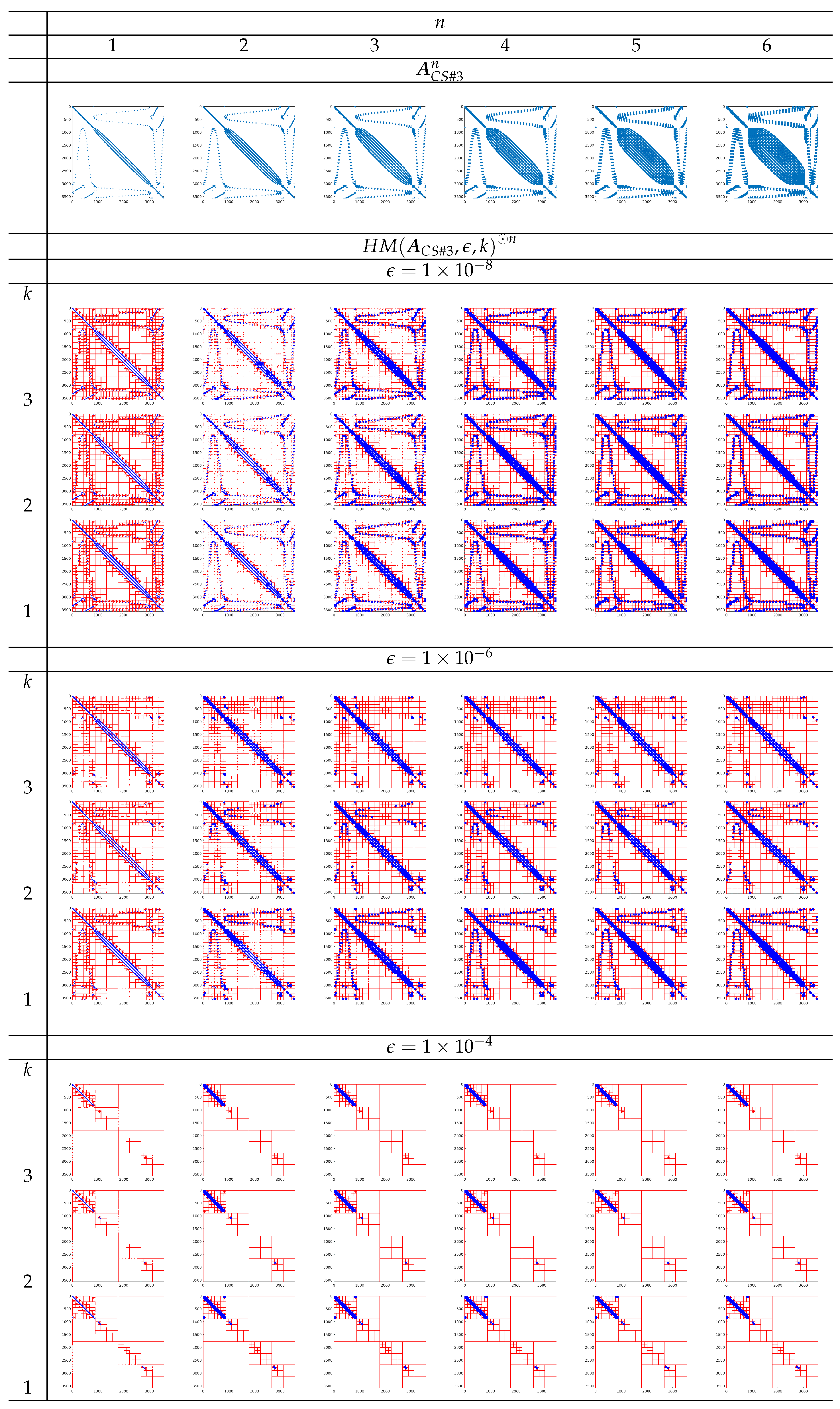
• Case Study #3 The matrix is obtained from the Harwell–Boeing Collection BCSSTK24 (BCS Structural Engineering Matrices) example (see [43] for details). The matrix ${\mathit{A}}_{CS\#3}\in {\Re }^{n\times n},n=3562$ is structured and sparse and its condition number in L2 norm is $\kappa \left({\mathit{A}}_{CS\#3}\right)=6.4e+11$. The sparsity pattern of ${\mathit{A}}_{CS\#3}$, and its first six n-powers $n=1,\dots ,6$, are presented in the first row of images in Figure 4.

All the considered matrices ${\mathit{A}}_{CS\#\left[1,2,3\right]}$ are scaled by the maximum value of the elements. From the first row of the images in Figure 2, Figure 3 and Figure 4, we can observe that the sparsity level of matrices decreases when the value of power degree n increases.

In Figure 2, Figure 3 and Figure 4, HM representations $HM{\left({\mathit{A}}_{CS\#\left[1,2,3\right]},ϵ,k\right)}^{\odot n}$ for the values of $ϵ=1e-8,1e-6,1e-4$, and $k=1,2,3$ of matrices ${\mathit{A}}_{CS\#\left[1,2,3\right]}$ are shown as a sparsity pattern, where red and blue colors, respectively, represent the admissible and inadmissible blocks. The admissible blocks are represented by red marking just the elements of each sub-block occupied by the elements of its rank-k approximation factors.

The presented results have the aim to

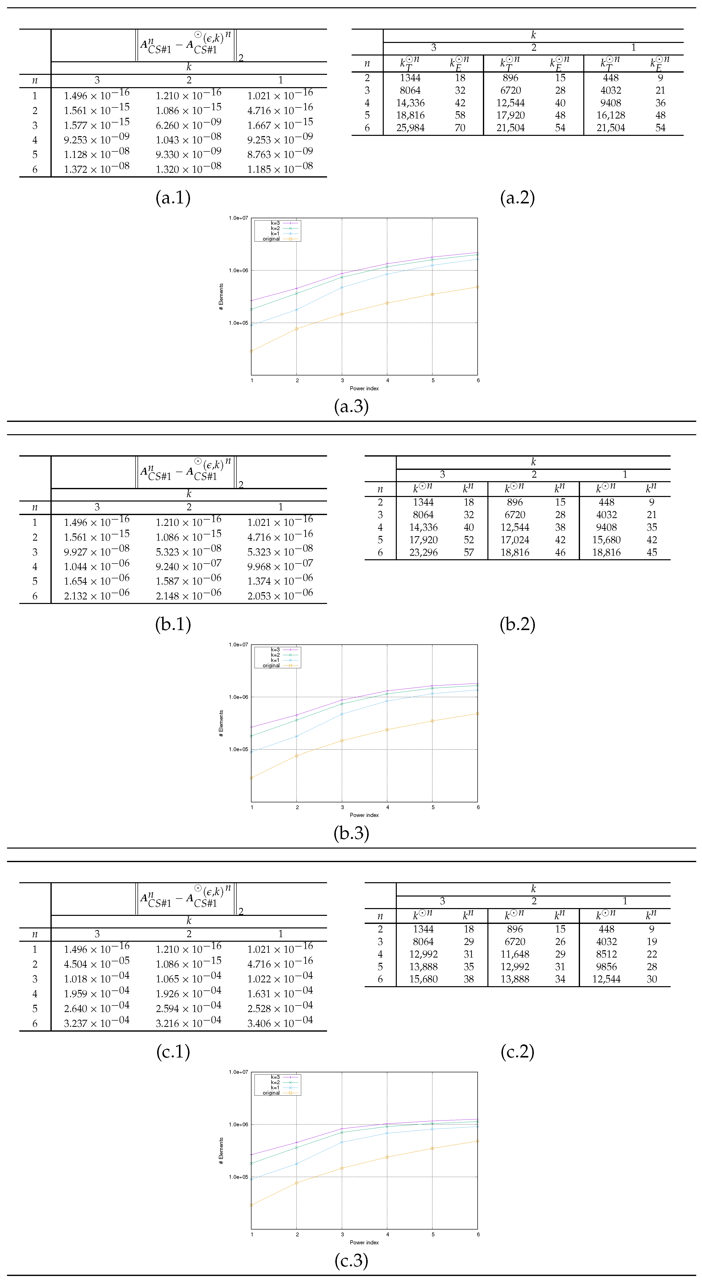
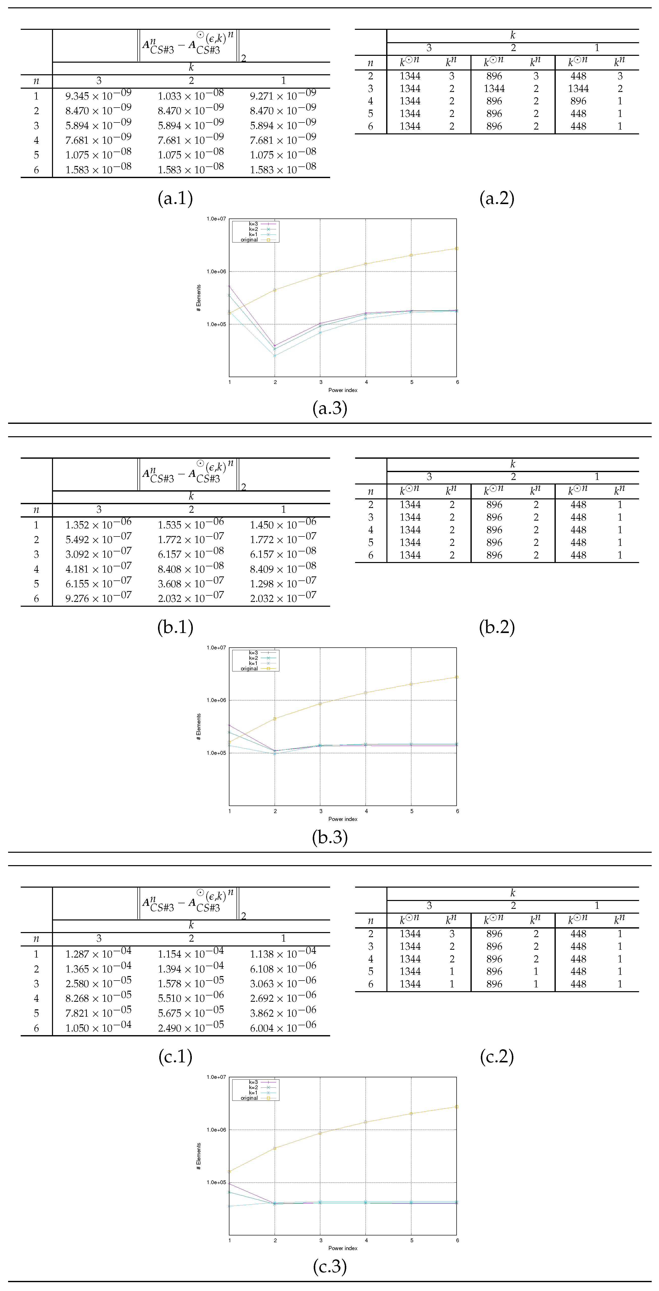
• evaluate the propagation of the error ${∥{\mathit{A}}_{CS\#\left[1,2,3\right]}^n-{\mathit{A}}_{CS\#\left[1,2,3\right]}^{{\odot }_{\left(ϵ,k\right)}n}∥}_2$ as a function of n, where ${\mathit{A}}_{CS\#\left[1,2,3\right]}^{{\odot }_{\left(ϵ,k\right)}n}$ denotes the natural representation of the HMs $HM{\left({\mathit{A}}_{CS\#\left[1,2,3\right]},ϵ,k\right)}^{\odot n}$ (see (a–c).1 in Figure 5, Figure 6 and Figure 7);
• compare the number $N_{{\mathit{A}}_{CS\#\left[1,2,3\right]}^n}$ of the nonzero elements needed to represent ${\mathit{A}}_{CS\#\left[1,2,3\right]}^n$ and the number $N_{HM{\left({\mathit{A}}_{CS\#\left[1,2,3\right]},ϵ,k\right)}^{\odot n}}$ of the total nonzero elements in both admissible and inadmissible blocks of $HM{\left({\mathit{A}}_{CS\#\left[1,2,3\right]},ϵ,k\right)}^{\odot n}$ (see (a–c).3 in Figure 5, Figure 6 and Figure 7);
• compare theoretical value $k_T^{\odot n}$ (obtained by repetitively applying the estimation (30)) with the effective value $k_E^{\odot n}$ (see (a–c).2 in Figure 5, Figure 6 and Figure 7). The value of $k_E^{\odot n}$ is determined at each step n as

  $$HM{\left({\mathit{A}}_{CS\#\left[1,2,3\right]},ϵ,k\right)}^{\odot n}=HM{\left({\mathit{A}}_{CS\#\left[1,2,3\right]},ϵ,k\right)}^{\odot n-1}HM\left({\mathit{A}}_{CS\#\left[1,2,3\right]},ϵ,k\right),$$

  (32)

  based on the following actions

  –

  after the computation of the product (32) by Algorithm 5, for each admissible block of $HM\left({\mathit{A}}_{CS\#\left[1,2,3\right]},ϵ,k\right)$ (identified by couple $\left(\tau ,\sigma \right)$ of indices sets), we compute the value $k_{\left(\tau ,\sigma \right)}^{\odot n}$ for which the corresponding block of $HM{\left({\mathit{A}}_{CS\#\left[1,2,3\right]},ϵ,k\right)}^{\odot n}$ can be considered admissible (with respect to $ϵ$ and $k_{\left(\tau ,\sigma \right)}^{\odot n}$);

  –

  we compute $k_E^{\odot n}$ as

  $$k_E^{\odot n}=\underset{\left(\tau ,\sigma \right)\in \mathfrak{A}}{max}{k}_{\left(\tau ,\sigma \right)}^{\odot n},$$

  where $\mathfrak{A}$ is the set of the admissible blocks of $HM\left({\mathit{A}}_{CS\#\left[1,2,3\right]},ϵ,k\right)$.

The sparsity pattern representation in Figure 2, Figure 3 and Figure 4 shows how admissible and inadmissible blocks are distributed. Such information should help to analyze which matrix structure is best suited, in terms of memory occupancy, for an HM representation.

From Figure 5, Figure 6 and Figure 7, several considerations can be drawn:

• the theoretical estimate $k_T^{\odot n}$ is a large overestimation of the actual value $k_E^{\odot n}$ computed in the operations (see plots (a–c).2 in Figure 5, Figure 6 and Figure 7);
• for all the $ϵ$ considered, the choice in k does not substantially modify the evolution of the error ${∥{\mathit{A}}_{CS\#\left[1,2,3\right]}^n-{\mathit{A}}_{CS\#\left[1,2,3\right]}^{{\odot }_{\left(ϵ,k\right)}n}∥}_2$ as n varies (see plots (a–c).1 in Figure 5, Figure 6 and Figure 7);
• since higher values of k imply a higher number of elements in the HM representation, it is convenient to choose the value of $k=1$ (see plots (a–c).3 in Figure 5, Figure 6 and Figure 7);
• some matrices seem to be more suitable than others for HM representation. In particular, it seems that matrices with a sparsity pattern that is not comparable to the one of a band matrix can be more effectively represented both in terms of the number of elements (for example, see the sparsity pattern for the matrices obtained from the Example Test #3 in Figure 4) and in terms of error evolution ${∥{\mathit{A}}_{CS\#1}^n-{\mathit{A}}_{CS\#1}^{{\odot }_{\left(ϵ,k\right)}n}∥}_2$.

From Figure 5, Figure 6 and Figure 7 and Figure 2, Figure 3 and Figure 4, we can deduce that, among the example matrices proposed, the one that guarantees the best performance in terms of memory occupancy is the matrix ${\mathit{A}}_{CS\#3}$. Indeed, the yellow line in plot (a–c).3 in Figure 7 almost always, depending on the value of $ϵ$, remains above the other lines in the same plot. We recall that the yellow line represents the trend, as a function of power degree n, of number $N_{{\mathit{A}}_{CS\#3}^n}$ of the nonzero elements needed to represent ${\mathit{A}}_{CS\#3}^n$; the other lines, each for different values of k, represent the number $N_{HM{\left({\mathit{A}}_{CS\#3},ϵ,k\right)}^{\odot n}}$ of the total nonzero elements in both admissible and inadmissible blocks of $HM{\left({\mathit{A}}_{CS\#3},ϵ,k\right)}^{\odot n}$. The same behavior is not observable for the other example matrices; indeed, for matrix ${\mathit{A}}_{CS\#1}$, the yellow line always remains below the other lines (see plot (a–c).3 in Figure 5); for matrix ${\mathit{A}}_{CS\#2}$, the yellow line sometimes remains above the other lines; generally, all lines are overlapping (see plot (a–c).3 in Figure 6). From images in Figure 4, we can observe that the admissible blocks concentrate near the diagonal, while the inadmissible blocks approximate the off-diagonal blocks with few elements the lower the required approximation precision $ϵ$ is (see images related to $ϵ=1\times {10}^{-4}$). The matrix ${\mathit{A}}_{CS\#3}$ has the best performance also in terms of preservation of the accuracy in HM representation of matrices. Such declaration is supported by error values reported in plots (a–c).1 in Figure 7 compared with the homologous tables in Figure 5 and Figure 6.

Figure 2. Sparsity representation for Example Test #1.

Figure 2. Sparsity representation for Example Test #1.

Figure 3. Sparsity representation for Example Test #2.

Figure 3. Sparsity representation for Example Test #2.

Figure 4. Sparsity representation for Example Test #3.

Figure 4. Sparsity representation for Example Test #3.

Figure 5. Results for Example Test #1: $ϵ=1\times {10}^{-8}$ (a), $ϵ=1\times {10}^{-6}$ (b), $ϵ=1\times {10}^{-4}$ (c). (a–c).1 Trend of the error ${∥{\mathit{A}}_{CS\#\left[1,2,3\right]}^n-{\mathit{A}}_{CS\#\left[1,2,3\right]}^{{\odot }_{\left(ϵ,k\right)}n}∥}_2$. (a–c).2 Trends of the numbers $k_T^{\odot n}$ and $k_E^{\odot n}$. (a–c).3 Trends of the numbers $N_{{\mathit{A}}_{CS\#\left[1,2,3\right]}^n}$ and $N_{HM{\left({\mathit{A}}_{CS\#\left[1,2,3\right]},ϵ,k\right)}^{\odot n}}$.

Figure 5. Results for Example Test #1: $ϵ=1\times {10}^{-8}$ (a), $ϵ=1\times {10}^{-6}$ (b), $ϵ=1\times {10}^{-4}$ (c). (a–c).1 Trend of the error ${∥{\mathit{A}}_{CS\#\left[1,2,3\right]}^n-{\mathit{A}}_{CS\#\left[1,2,3\right]}^{{\odot }_{\left(ϵ,k\right)}n}∥}_2$. (a–c).2 Trends of the numbers $k_T^{\odot n}$ and $k_E^{\odot n}$. (a–c).3 Trends of the numbers $N_{{\mathit{A}}_{CS\#\left[1,2,3\right]}^n}$ and $N_{HM{\left({\mathit{A}}_{CS\#\left[1,2,3\right]},ϵ,k\right)}^{\odot n}}$.

Figure 6. Results for Example Test #2: $ϵ=1\times {10}^{-8}$ (a), $ϵ=1\times {10}^{-6}$ (b), $ϵ=1\times {10}^{-4}$ (c). (a–c).1 Trend of the error ${∥{\mathit{A}}_{CS\#\left[1,2,3\right]}^n-{\mathit{A}}_{CS\#\left[1,2,3\right]}^{{\odot }_{\left(ϵ,k\right)}n}∥}_2$. (a–c).2 Trends of the numbers $k_T^{\odot n}$ and $k_E^{\odot n}$. (a–c).3 Trends of the numbers $N_{{\mathit{A}}_{CS\#\left[1,2,3\right]}^n}$ and $N_{HM{\left({\mathit{A}}_{CS\#\left[1,2,3\right]},ϵ,k\right)}^{\odot n}}$.

Figure 6. Results for Example Test #2: $ϵ=1\times {10}^{-8}$ (a), $ϵ=1\times {10}^{-6}$ (b), $ϵ=1\times {10}^{-4}$ (c). (a–c).1 Trend of the error ${∥{\mathit{A}}_{CS\#\left[1,2,3\right]}^n-{\mathit{A}}_{CS\#\left[1,2,3\right]}^{{\odot }_{\left(ϵ,k\right)}n}∥}_2$. (a–c).2 Trends of the numbers $k_T^{\odot n}$ and $k_E^{\odot n}$. (a–c).3 Trends of the numbers $N_{{\mathit{A}}_{CS\#\left[1,2,3\right]}^n}$ and $N_{HM{\left({\mathit{A}}_{CS\#\left[1,2,3\right]},ϵ,k\right)}^{\odot n}}$.

Figure 7. Results for Example Test #3: $ϵ=1\times {10}^{-8}$ (a), $ϵ=1\times {10}^{-6}$ (b), $ϵ=1\times {10}^{-4}$ (c). (a–c).1 Trend of the error ${∥{\mathit{A}}_{CS\#\left[1,2,3\right]}^n-{\mathit{A}}_{CS\#\left[1,2,3\right]}^{{\odot }_{\left(ϵ,k\right)}n}∥}_2$. (a–c).2 Trends of the numbers $k_T^{\odot n}$ and $k_E^{\odot n}$. (a–c).3 Trends of the numbers $N_{{\mathit{A}}_{CS\#\left[1,2,3\right]}^n}$ and $N_{HM{\left({\mathit{A}}_{CS\#\left[1,2,3\right]},ϵ,k\right)}^{\odot n}}$.

Figure 7. Results for Example Test #3: $ϵ=1\times {10}^{-8}$ (a), $ϵ=1\times {10}^{-6}$ (b), $ϵ=1\times {10}^{-4}$ (c). (a–c).1 Trend of the error ${∥{\mathit{A}}_{CS\#\left[1,2,3\right]}^n-{\mathit{A}}_{CS\#\left[1,2,3\right]}^{{\odot }_{\left(ϵ,k\right)}n}∥}_2$. (a–c).2 Trends of the numbers $k_T^{\odot n}$ and $k_E^{\odot n}$. (a–c).3 Trends of the numbers $N_{{\mathit{A}}_{CS\#\left[1,2,3\right]}^n}$ and $N_{HM{\left({\mathit{A}}_{CS\#\left[1,2,3\right]},ϵ,k\right)}^{\odot n}}$.

All the proposed algorithms related to basic linear algebra operations based on the HM representation can be easily parallelized, due to their recursive formulation, by distributing computations across the different components of the computing resource hierarchy. As an example, we report in Algorithm 6 a possible parallel implementation of Algorithm 3.

Algorithm 6 Parallel matrix–vector multiplication $\mathit{y}=\mathit{y}+\mathit{A}\mathit{x}$ of the $\mathcal{H}$-matrix of blockwise rank k $\mathit{A}\in {\Re }^{I\times I}$ (defined on block cluster quad-tree ${\mathcal{T}}_{I\times I}\left(L\right)$) with vector $x\in {\Re }^I$. The index sets $\tau \times \sigma$ to be used in the first call to the recursive ParHMatrix-MVM procedure are such that $\tau =\sigma =I$.

1: procedure ParHMatrix-MVM($\mathit{A}$, $\mathit{y}$, $\mathit{x}$, ${\mathcal{T}}_{I\times I}\left(L\right)$, $\tau \times \sigma$)   2: Input: $\mathit{A}$, $\mathit{y}$, $\mathit{x}$, ${\mathcal{T}}_{I\times I}\left(L\right)$, $\tau \times \sigma$   3: Output:  $\mathit{y}$   4:     if $S\left(\tau \times \sigma \right)\ne \varnothing$ then     ▹$\tau \times \sigma$ is not a leaf of ${\mathcal{T}}_{I\times I}\left(L\right)$   5:         parallel for each ${\tau }^{\prime }\times {\sigma }^{\prime }\in S\left(\tau \times \sigma \right)$ do num_tasks ($N_{Tasks}$) reduction(+:$\mathit{y}$)   6:            ParHMatrix-MVM($\mathit{A}$, $\mathit{y}$, $\mathit{x}$, ${\mathcal{T}}_{I\times I}\left(L\right)$, ${\tau }^{\prime }\times {\sigma }^{\prime }$)   7:         end parallel for   8:     else ▹$\tau \times \sigma$ is a leaf of ${\mathcal{T}}_{I\times I}\left(L\right)$, then execute the GEMV BLAS2 operation ${\mathit{y}}_{\left|\tau \right.}\leftarrow {\mathit{y}}_{\left|\tau \right.}+{\mathit{A}}_{\left|\tau \times \sigma \right.}{\mathit{x}}_{\left|\sigma \right.}$   9:         if (${\mathit{A}}_{\left|\tau \times \sigma \right.}{\mathit{x}}_{\left|\sigma \right.}$ is admissible) then 10:            $\alpha \leftarrow 1$ 11:            $\beta \leftarrow 0$ 12:            $\mathit{z}\leftarrow$GEMV($\alpha$, ${\mathbf{\Sigma }}_{\left|\tau \times \sigma \right.}{\mathit{V}}_{\left|\tau \times \sigma \right.}^T$, ${\mathit{x}}_{\left|\sigma \right.}$, $\beta$, $\mathit{z}$, $DeviceType$) 13:            $\beta \leftarrow 1$ 14:            ${\mathit{y}}_{\left|\tau \right.}\leftarrow$GEMV($\alpha$, ${\mathit{U}}_{\left|\tau \times \sigma \right.}$, $\mathit{z}$, $\beta$, ${\mathit{y}}_{\left|\tau \right.}$, $DeviceType$) 15:         else 16:            $\alpha \leftarrow 1$ 17:            $\beta \leftarrow 1$ 18:            ${\mathit{y}}_{\left|\tau \right.}\leftarrow$GEMV($\alpha$,${\mathit{A}}_{\left|\tau \times \sigma \right.}$,${\mathit{x}}_{\left|\sigma \right.}$,$\beta$,${\mathit{y}}_{\left|\tau \right.}$,$DeviceType$) 19:         end if 20:     end if 21: end procedure

The pseudocode listed borrows the constructs used by tools such as OpenMP [44]: in particular, it uses the parallel for construct to indicate the distribution of the instructions included in its body among $N_{Tasks}$ concurrent tasks, while the reduction instruction indicates that the different outputs of the vector $\mathit{y}$ must be added together at the end of the cycle.

The value of variable $N_{Tasks}^{\left(l\right)}$, at each level l of the block cluster quad-tree ${\mathcal{T}}_{I\times I}\left(L\right)$, is assumed to be such that $N_{Tasks}^{\left(l\right)}\le C\left(\tau \times \sigma \right)$, where $C\left(\tau \times \sigma \right)=\left|S\left(\tau \times \sigma \right)\right|$ is the cardinality of the set of sons of the index subset $\tau \times \sigma$. If the value of $N_{Tasks}^{\left(l\right)}$ divides such cardinality, at most, $N_{Tasks}^{\left(l\right)}$ tasks are spawned, and each task executes $C\left(\tau \times \sigma \right)/N_{Tasks}^{\left(l\right)}$ new call to ParHMatrix-MVM procedure. If $N_{Tasks}^{\left(l\right)}=1$, the execution of the l-th level of Algorithm 6 coincides with that of Algorithm 3.

We recall that BLAS (Basic Linear Algebra Subprograms) are a set of routines [45] that provide optimized standard building blocks for performing primary vector and matrix operations. BLAS routines can be classified depending on the types of operands: Level 1: operations involving just vector operands; Level 2: operations between vectors and matrices; and Level 3: operations involving just matrix operands. The operation $\mathit{y}=\beta \mathit{y}+\alpha \mathit{A}\mathit{x}$ is called a GEMV operation when $\mathit{A}$, $\mathit{x}$, $\mathit{y}$, $\alpha ,$ and $\beta$ are, respectively, a matrix, two vectors, and two scalars.

The GEMV BLAS2 operation needed at lines 12 and 14 and 18 in Algorithm 6 is implemented by using the most effective component (identified by the macro $DeviceType$) of the computing architecture by a call to optimized mathematical software libraries available for that component (for example, the multithread version of the Intel MKL [46] library or the cuBLAS [47] library when using, as $DeviceType$, respectively, the Intel CPUs or the NVIDIA GP-GPU accelerators. All the issues related to the most efficient memory hierarchy accesses are delegated to such optimized versions of the BLAS procedures.

In Figure 8, an example of the execution tree of Algorithm 6 is shown. In the left part of Figure 8, the block structure of the $\mathcal{H}$-matrix $\mathit{A}$ is defined on block cluster quad-tree ${\mathcal{T}}_{I\times I}\left(L\right)$, where $L=2$ is represented. The admissible and inadmissible blocks are represented, respectively, by yellow and red boxes. In the execution tree of Algorithm 6 (see the right part of Figure 8) the leaves are represented by a green box. At each of the two levels of the tree, the considered value for $N_{Tasks}^{\left(l\right)}$ is $N_{Tasks}^{\left(l\right)}=4,l=0,1$. The following steps are executed:

• Starting from level $l=0$, $N_{Tasks}^{\left(0\right)}$ concurrent tasks are spawned, the task with identification number $I{d}^{\left(0\right)}=2$ is related to a leaf, and then, the block being an admissible one, there is the procedure compute contribution to the sub-block of vector $\mathit{y}$ related to the index subset ${\tau }_1^{\left(1\right)}$ by code at lines 12 and 14 of Algorithm 6. Each of the remaining tasks execute a parallel for each spawning other $N_{Tasks}^{\left(1\right)}$ concurrent tasks executing at the following level $l=2$, with a total of $3N_{Tasks}^{\left(1\right)}=12$ concurrent tasks.
• At the level $l=2$, all the block are leaves. If the blocks are admissible, they are used to compute contributions to the sub-blocks of vector $\mathit{y}$ by code at the lines 12 and 14 of Algorithm 6; otherwise, the same sub-blocks are updated by code at the line 18. In particular, assuming that the variable $I{d}_{\left(I{d}^{\left(l-1\right)}\right)}^{\left(l\right)}$ is used to represent the task identification number of a task spawned at the level l by a task with identifier, at the $l-1$-th level, $I{d}^{\left(l-1\right)}$,

  –

  tasks with identification numbers $I{d}_{\left(1\right)}^{\left(1\right)}=1,2$ compute contributions to sub-blocks of $\mathit{y}$ related to the index subset ${\tau }_1^{\left(2\right)}$ and tasks with identification numbers $I{d}_{\left(1\right)}^{\left(1\right)}=3,4$ update sub-blocks of $\mathit{y}$ related to the index subset ${\tau }_2^{\left(2\right)}$. Then, all the tasks spawned from task $I{d}^{\left(0\right)}=1$ (see Figure 8(b.1)) compute contributions to sub-blocks of $\mathit{y}$ related to the index subset ${\tau }_1^{\left(1\right)}$.

  –

  In the same way, tasks with identification numbers $I{d}_{\left(3\right)}^{\left(1\right)}=1,2$ compute contributions to sub-blocks of $\mathit{y}$ related to the index subset ${\tau }_3^{\left(2\right)}$, and tasks with identification numbers $I{d}_{\left(3\right)}^{\left(1\right)}=3,4$ compute contributions to sub-blocks of $\mathit{y}$ related to the index subset ${\tau }_4^{\left(2\right)}$. Then, all the tasks spawned from task $I{d}^{\left(0\right)}=3$ (see Figure 8(b.2)) compute contributions to sub-blocks of $\mathit{y}$ related to the index subset ${\tau }_2^{\left(1\right)}$.

  –

  In the same way, the tasks with identification numbers $I{d}_{\left(4\right)}^{\left(1\right)}=1,2,3,4$ (see Figure 8(b.3)) also compute contributions to sub-blocks of $\mathit{y}$ related to the index subset ${\tau }_2^{\left(1\right)}$.

• At the termination of parallel for at level $l=1,0$, the contributions to sub-blocks of $\mathit{y}$ related to the index subset ${\tau }_1^{\left(1\right)}$ and ${\tau }_2^{\left(1\right)}$ are summed together (by means of the reduce operation) to obtain the final status for vector $\mathit{y}$.

3. Matrix Polynomial Evaluation

Let $p_n\left(\mathit{A}\right)$ be a real polynomial of degree n of the matrix $\mathit{A}\in {\Re }^{M\times M}$, where the set ${\left\{{\alpha }_i:{\alpha }_i\in \Re \right\}}_{i=0,\dots ,n}$ is the set of its coeffients.

$$p_n\left(\mathit{A}\right)=\sum _{i=0}^n{\alpha }_i{\mathit{A}}^i.$$

(33)

Different methods can be used to evaluate polynomials defined by Equation (33) [1]. We propose the one of Paterson and Stockmeyer [48] in which $p_m\left(\mathit{A}\right)$ is written as

$$p_n\left(\mathit{A}\right)=\sum _{k=0}^r{\mathit{B}}_k{\left({\mathit{A}}^s\right)}^k,r=\lfloor n/s\rfloor$$

(34)

where s is an integer parameter and

$${\mathit{B}}_k=\sum _{i=0}^{s_k}{\alpha }_{sk+i}{\mathit{A}}^i,\mathrm{where}{s}_k=\left\{\begin{array}{ccc}s-1& \mathrm{if}& k<r\\ n-rs& \mathrm{if}& k=r\end{array}\right.$$

(35)

After the powers ${\mathit{A}}^i,i=1,\dots ,s$ are computed, polynomials defined in Equation (34) can be evaluated by Horner’s method [1], where each ${\mathit{B}}_k$ is formed when needed.

The two extreme cases, $s=1$ and $s=n$, reduce, respectively, to Horner’s method and to the method that evaluates polynomials via explicit powers.

The total cost $TCPS\left(s,r,M\right)$ of the polynomial evaluation is

$$T{C}_{PS}\left(s,r,M\right)=\left(s+r-1-f\left(r\right)\right)MC\left(M\right),$$

(36)

where

$$f\left(r\right)=\left\{\begin{array}{ccc}1\hfill & \mathrm{if}\hfill & r=0\hfill \\ 0\hfill & \mathrm{otherwise}\hfill \end{array}\right.,$$

(37)

and where $MC\left(M\right)$ denotes the computational cost of a matrix multiplication $\mathit{A}\mathit{B}$ with $\mathit{A},\mathit{B}\in {\Re }^{M\times M}$.

$T{C}_{PS}\left(s,r,M\right)$, defined as in Equation (36), is approximately minimized by $q=\sqrt{n}$. From Equation (36), we can argue that the described method requires much less work than other ones, such as Horner’s method (whose computational cost is $T{C}_H\left(n,M\right)=\left(n-1\right)MC\left(M\right)$), for large q.

In Algorithm 7, a procedure for matrix polynomial evaluation based on Paterson and Stockmeyer method is presented. The version of Algorithm 7 based on HM representation of involved matrices, and hence on the algorithms introduced in Section 2, is listed in Algorithm 8.

Algorithm 7 Procedure for matrix polynomial evaluation based on Paterson and Stockmeyer method. $\mathit{A}$ and $\mathit{P}$ represent, respectively, the matrix and the results of Equation (33). n represents the degree of the polynomial and $\alpha$ the vector of the polynomial coefficients ${\left[{\alpha }_i\right]}_{i=0,\dots ,n}$.

1: procedure MatPolyEvaluation($\mathit{A}$, $\mathit{P}$, $\alpha$, n, s)   2: Input: $\mathit{A}$, $\alpha$, n, s   3: Output:  $\mathit{P}$   4:     $r\leftarrow$ Compute $r=\lfloor {\displaystyle \frac{n}{s}}\rfloor$ ▹ Compute and store the first s powers of $\mathit{A}$   5:     for $i=0,\dots ,s$ do   6:         $PowS\left[i\right]\leftarrow {\mathit{A}}^i$   7:     end for ▹ Compute and store the first r powers of ${\mathit{A}}^s$   8:     for $k=0,\dots ,r$ do   9:         $PowR\left[k\right]\leftarrow PowS{\left[s\right]}^k$ 10:         $t\left[k\right]\leftarrow$ Compute $t\left[k\right]=\left(k<r\right)?s-1:n-rs$ 11:     end for ▹ Compute and store ${\mathit{B}}_k,k=0,\dots ,r$ 12:     for $k=0,\dots ,r$ do 13:         $Bk\left[k\right]\leftarrow \mathbf{0}$ 14:         for $\mathit{i}=0,\dots ,t\left[k\right]$ do 15:            $Bk\left[k\right]\leftarrow$ Compute $Bk\left[k\right]=Bk\left[k\right]+\alpha \left[sk+i\right]PowS\left[i\right]$ 16:         end for 17:     end for ▹ Compute $\mathit{P}$ 18:     $\mathit{P}\leftarrow \mathbf{0}$ 19:     for $k=0,\dots ,r$ do 20:         $\mathit{P}\leftarrow$ Compute $\mathit{P}=\mathit{P}+Bk\left[k\right]PowR\left[k\right]$ 21:     end for 22: end procedure

To evaluate Algorithm 8, where the involved matrices have an HM representation, we performed some tests using the same case studies described in the previous Section 2. The coefficients of the polynomial are generated randomly due to a uniform distribution in the interval $\left[0,1\right]$.

The presented results (see

Table 2. Polynomial evaluation test results: list of the errors $E\left({\mathit{A}}_{CS\#\left[1,2,3\right]},n,s\right)$ as a function of the polynomial degree n.

n	$\mathit{E}\left({\mathit{A}}_{\mathit{CS}\#1},\mathit{n},\mathit{s}\right)$	$\mathit{E}\left({\mathit{A}}_{\mathit{CS}\#2},\mathit{n},\mathit{s}\right)$	$\mathit{E}\left({\mathit{A}}_{\mathit{CS}\#3},\mathit{n},\mathit{s}\right)$
10	$3.454\times {10}^{-08}$	$3.688\times {10}^{-08}$	$7.153\times {10}^{-08}$
14	$7.092\times {10}^{-08}$	$1.690\times {10}^{-07}$	$6.179\times {10}^{-07}$
18	$1.019\times {10}^{-07}$	$2.226\times {10}^{-06}$	$2.344\times {10}^{-06}$
22	$1.394\times {10}^{-07}$	$1.055\times {10}^{-05}$	$1.383\times {10}^{-05}$

) have the aim to show the evolution of the errors $E\left({\mathit{A}}_{CS\#\left[1,2,3\right]},n,s\right)$, as a function of the polynomial degree n, for the fixed value of $s=4$, where

$$E\left({\mathit{A}}_{CS\#\left[1,2,3\right]},n,s\right)={∥p_n\left({\mathit{A}}_{CS\#\left[1,2,3\right]},s\right)-p_n^{\odot }\left(HM\left({\mathit{A}}_{CS\#\left[1,2,3\right]},ϵ,k\right),s\right)∥}_2,$$

(38)

and where the symbols $p_n\left({\mathit{A}}_{CS\#\left[1,2,3\right]},s\right)$ and $p_n^{\odot }\left(HM\left({\mathit{A}}_{CS\#\left[1,2,3\right]},ϵ,k\right),s\right)$ represent

• $p_n\left({\mathit{A}}_{CS\#\left[1,2,3\right]},s\right)$: the evaluation of the polynomial (33) through Algorithm 8 for the matrix ${\mathit{A}}_{CS\#\left[1,2,3\right]}$;
• $p_n^{\odot }\left(HM\left({\mathit{A}}_{CS\#\left[1,2,3\right]},ϵ,k\right),s\right)$: the natural representation of the evaluation of the polynomial (33) by means of Algorithm 8, where the involved matrices have an HM representation. In such a case, all the operations involving matrices (summation, product, and exponentiation) are based on Algorithms 2 and 5. In the summation operations, $\mathit{C}=\mathit{A}{\oplus }_{k_C}\mathit{B}$, the value $k_C$ of the result $\mathit{C}$ is computed as the maximum value between the values $k_A$ and $k_B$ of the operands $\mathit{A}$ and $\mathit{B}$.

Algorithm 8 Procedure for matrix polynomial evaluation based on Paterson and Stockmeyer method based on HM representation of involved matrices (defined on block cluster quad-tree ${\mathcal{T}}_{I\times I}\left(L\right)$). $\mathit{HMA}$ and $\mathit{HMP}$ represent, respectively, the HM representation of the matrix $\mathit{A}$ and the results $\mathit{P}$ of Equation (33). n represents the degree of the polynomial and $\alpha$ the vector of the polynomial coefficients ${\left[{\alpha }_i\right]}_{i=0,\dots ,n}$.

1: procedure MatPolyEvaluation($\mathit{HMA}$, $\mathit{HMP}$, $\alpha$, n, s)   2: Input: $\mathit{HMA}$, $\alpha$, n, s   3: Output:  $\mathit{HMP}$   4:     $r\leftarrow$ Compute $r=\lfloor {\displaystyle \frac{n}{s}}\rfloor$ ▹ Compute and store the first s powers of $\mathit{A}$   5:     $HMPowS\left[1:s\right]\leftarrow$HMatrix-Power($\mathit{HMA}$, s) ▹ Compute and store the first r powers of ${\mathit{A}}^s$   6:     $HMPowR\left[1:r\right]\leftarrow$HMatrix-Power($HMPowS\left[s\right]$,r)   7:     for $k=0,\dots ,r$ do   8:         $s\left[k\right]\leftarrow$ Compute $s\left(k\right]=\left(k<r\right)?s-1:n-rs$   9:     end for ▹ Compute and store ${\mathit{B}}_k,k=0,\dots ,r$ 10:     for $k=0,\dots ,r$ do 11:         $HMBk\left[k\right]\leftarrow \mathbf{0}$ 12:         for $\mathit{i}=0,\dots ,s\left[k\right]$ do ▹ Compute scaled matrix $\mathit{HMC}=\alpha \left[sk+i\right]HMPowS\left[i\right]$ by Algorithm 4 13:            HMatrix-MScale($HMPowS\left[i\right]$, $\alpha \left[sk+i\right]$, $\mathit{HMC}$) ▹ Compute $HMBk\left[k\right]$ by an iterative updating using Algorithm 2 14:            HMatrix-MSum($HMBk\left[k\right]$, $\mathit{HMC}$, $HMBk\left[k\right]$, ${\mathcal{T}}_{I\times I}\left(L\right)$, I, I) 15:         end for 16:     end for ▹ To compute $\mathit{P}$, consecutively apply (for $r+1$ times) Algorithm 5. At each step, the value of $K^{\odot }$ is computed as already described for Equation (32). The value of $K^{\oplus }$ is computed as the maximum value between the values of $K_C$ and $K_{AB}$. 17:     $\mathit{HMP}\leftarrow \mathbf{0}$ 18:     for $k=0,\dots ,r$ do 19:         HMatrix-MMMult($HMBk\left[k\right]$, $HMPowR\left[k\right]$, $\mathit{HMP}$, ${\mathcal{T}}_{I\times I}\left(L\right)$, I, I) 20:     end for 21: end procedure       22: function HMatrix-Power($\mathit{HMA}$, s) 23: Input: $\mathit{HMA}$, s 24:     $HMAPOWS\left[1\right]\leftarrow \mathit{HMA}$ ▹ Consecutively apply (for $s-1$ times) Algorithm 5. At each step, the value of $K^{\odot }$ is computed as already described for Equation (32) 25:     for $\mathit{i}=2,\dots ,s$ do 26:         $HMAPOWS\left[i\right]\leftarrow \mathbf{0}$ 27:         HMatrix-MMMult($\mathit{HMA}$, $HMAPOWS\left[i-1\right]$, $HMAPOWS\left[i\right]$, ${\mathcal{T}}_{I\times I}\left(L\right)$, I, I) 28:     end for 29:     return $HMAPOWS\left[1:s\right]$ 30: end function

From Table 2, it can be observed that the evolution of the errors $E\left({\mathit{A}}_{CS\#\left[1,2,3\right]},n,s\right)$, as a function of the polynomial degree n, seems to be sufficiently sensitive to the matrix type even with the risk that such errors may explode. Such behavior can have serious consequences on the results of operations involving such kinds of polynomials. It is the case of the example shown in the case study described in Section 4, where the result of a matrix polynomial evaluation is used in a matrix–vector operation of the kind $\mathit{A}\mathit{b}=\mathit{c}$. If we denote by $\delta \mathit{A}$ the error in representing $\mathit{A}$ and by $\mathit{c}-\delta \mathit{c}$ the results of the operation $\left(\mathit{A}-\delta \mathit{A}\right)\mathit{b}$, then we have

$$\begin{array}{ccc}\hfill {\displaystyle \frac{{∥\delta \mathit{c}∥}_2}{{∥\mathit{c}∥}_2}}& =& {\displaystyle \frac{\left({∥\delta \mathit{c}∥}_2-{∥\mathit{c}∥}_2\right)+{∥\mathit{c}∥}_2}{{∥\mathit{c}∥}_2}}\hfill \\ & \le & 1+{\displaystyle \frac{{∥\mathit{c}-\delta \mathit{c}∥}_2}{{∥\mathit{c}∥}_2}}=1+{\displaystyle \frac{{∥\left(\mathit{A}-\delta \mathit{A}\right)\mathit{b}∥}_2}{{∥\mathit{c}∥}_2}}\hfill \\ & \le & 2+{∥\delta \mathit{A}∥}_2{\displaystyle \frac{{∥\mathit{b}∥}_2}{{∥\mathit{c}∥}_2}}\hfill \end{array}$$

(39)

Therefore, from (39), it follows that the relative error ${\displaystyle \frac{{∥\delta \mathit{c}∥}_2}{{∥\mathit{c}∥}_2}}$ of the results of perturbed matrix–vector operation has an upper limit depending on the norm of the error on matrix $\delta \mathit{A}$. So, if $\delta \mathit{A}$ has a large value, ${\displaystyle \frac{{∥\delta \mathit{c}∥}_2}{{∥\mathit{c}∥}_2}}$ also potentially has a large value.

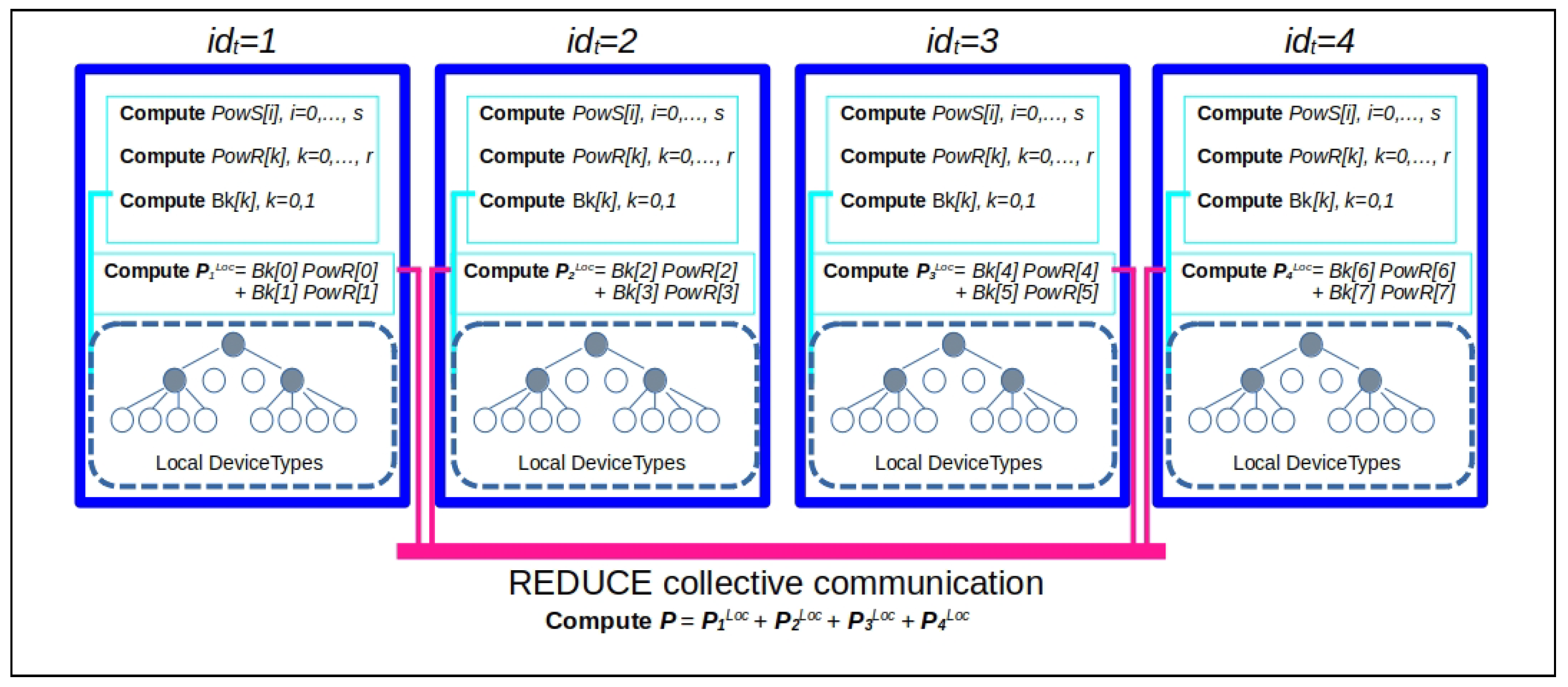
Algorithm 7 for matrix polynomial evaluation based on Paterson and Stockmeyer method (and then Algorithm 8, which is its HM-based variant) lends itself well to parallel implementations; for example, if we imagine dividing the r matrix $Bk\left(k\right),k=1,\dots ,r$ among $N_{Tasks}$ concurrent tasks, then

• the s matrices $PowS\left(i\right),i=0,\dots ,s$ and the r matrices $PowR\left(i\right),k=0,\dots ,r$ (see lines 6 and 9 of Algorithm 7) could be computed by all the $N_{Tasks}$ tasks concurrently and independently of each other (no communications are needed among tasks);
• during the update phase of polynomial $\mathbf{P}$ (see line 20 of Algorithm 7), the local update of $\mathbf{P}$ on each task $i{d}_t$ can be performed concurrently (no communications are needed among tasks). To complete the computation of $\mathbf{P}$, just one collective communication is needed at the end of the algorithm.

Furthermore, every call to a function/procedure of the kind HMatrix-* in Algorithm 8 can be executed by each task using a locally available type of concurrency (a set of CPUs, cores, or accelerators) and fully exploiting the hierarchy of processing units (see Algorithm 6 for an example of such a strategy).

In Figure 9, we show an example of parallel implementation of Algorithm 7 (and then of Algorithm 8) by $N_{Tasks}=4$ and $r=7$. Each task may mapped to a node holding devices such as CPUs and accelerators. The computation of operations involving HM can be locally executed by an execution tree such as those shown in Figure 8.

4. A Case Study in Graph Convolutional Deep Neural Network Applications

As very effective tools for learning on graph-structured data (that stands for building a data-driven model from the same data), Graph Neural Networks (GNNs) have shown cutting-edge performance in a variety of applications, including biological network modeling and social network analysis. Compared to analyzing data separately, the special capability of graphs to capture the structural relationships between data allows for the extraction of additional insights. Among the GNNs, Graph Convolutional Deep Neural Network [49] appears as one of the most prominent graph deep learning models [50].

4.1. Introduction to Graph Convolutional Deep Neural Network

Graph Convolutional Deep Neural Networks are based on the theory of Spectral Analysis of a graph [50,51,52,53]. Spectral graph theory is the field concerned with the study of the eigenvectors and eigenvalues of the matrices that are naturally associated with graphs. One of the goals is to determine important properties of the graph from its graph spectrum.

Apart from theoretical interest, spectral graph theory also has a wide range of applications. Among them, we have to cite the construction of graph filters that are defined in the context of Discrete Signal Processing on Graphs ($DS{P}_G$), whose aim is to represent, process, and analyze structured datasets that can be represented by graphs [52,54,55].

Let us introduce some definitions.

Definition 5 

(Signal defined on a weighted undirected graph $\mathit{G}$). A weighted undirected graph $\mathit{G}$ is a triple $\left(\mathit{N},\mathit{E},\mathit{w}\right)$, where $\mathit{N}=\left\{n_1,\dots ,n_{N_{nodes}}\right\}$ is the set of $N_{nodes}$ nodes and $\mathit{E}$ is the set of $N_{edges}$ edges. An edge $e_{\left(i,j\right)}\in \mathit{E}$ is a couple of index $\left(i,j\right)$ such that nodes $n_i$ and $n_j$ are considered connected in graph $\mathit{G}$.

The set $\mathit{w}=\left\{w_{i,j},\left(i,j\right)\in \mathit{E}\right\}$ of $N_{edges}$ values is called the set of weights of $\mathit{G}$, where

$$\begin{array}{ccc}\hfill w_{i,j}& >& 0\hfill \\ \hfill w_{i,j}& =& w_{j,i}.\hfill \end{array}$$

The matrix $\mathit{A}={\left(a_{i,j}\right)}_{i,j=1,\dots ,N_{nodes}}$ is the weighted adjacency matrix of the graph $\mathit{G}$ if

$$a_{i,j}=\left\{\begin{array}{cc}{w}_{i,j}\hfill & if\left(i,j\right)\in \mathit{E},\hfill \\ 0\hfill & otherwise.\hfill \end{array}\right.$$

(40)

Assuming, without a loss of generality, that dataset elements are real scalars, we define a graph signal as a map $\mathit{s}$ from the set $\mathit{N}$ of nodes in the set of real numbers ℜ:

$$\mathit{s}:n_i\in \mathit{N}\mapsto s_i\in \Re$$

(41)

For simplicity of discussion, we write graph signals as vectors $s={\left(s_i,i=1,\dots ,N_{nodes}\right)}^T$.

Definition 6 

(Linear filters for signal defined on a weighted undirected graph $\mathit{G}$). A function $h:\mathit{s}\in \mathit{N}\mapsto h\left(\mathit{s}\right)\in \mathit{N}$ is called a filter on a graph $\mathit{G}$. A filter h on a graph $\mathit{G}$ is called a Linear Filter if a matrix $\mathit{H}$ exists such that

$$h\left(\mathit{s}\right)=\mathit{H}\mathit{s}.$$

(42)

Definition 7 

(Graph Fourier Transform of a signal defined on a weighted undirected graph $\mathit{G}$). Let us define the Graph Laplacian matrix $\mathit{L}\in {\Re }^{N_{nodes}\times N_{nodes}}$ of the weighted undirected graph $\mathit{G}$ as the following symmetric positive semidefinite matrix:

$$\mathit{L}=\mathit{D}-\mathit{A},$$

(43)

where $\mathit{D}=diag\left(\mathit{d}\right)\in {\Re }^{N_{nodes}\times N_{nodes}}$ is a diagonal matrix whose diagonal vector $\mathit{d}={\left(d_i\right)}_{i=1,\dots ,N_{nodes}}$ is defined as

$$d_i=\sum _{j=1}^{N_{nodes}}{A}_{i,j}$$

(44)

Matrix $\mathit{D}$ is called degree matrix. In some cases, the Symmetric Normalized Laplacian is defined as

$${\mathit{L}}_{SymNorm}={\mathit{D}}^{-1/2}\mathit{L}{\mathit{D}}^{-1/2}$$

(45)

Let us consider the singular value decomposition (SVD) [38] of the Laplacian matrix $\mathit{L}$; then, due to the properties of $\mathit{L}$, such decomposition can be written as

$$\mathit{L}=\mathit{U}\mathbf{\Lambda }{\mathit{U}}^T$$

(46)

where the set of the columns ${\left\{{\mathit{u}}^j\right\}}_{i=1,\dots ,N_{nodes}}$ of the matrix $\mathit{U}$ are a set of orthonormal vectors called Graph Fourier Modes and where the diagonal elements ${\left\{{\lambda }_i\right\}}_{i=1,\dots ,N_{nodes}}$ of the diagonal matrix Λ are non-negative and are identified as the frequencies of the graph.

Following Shuman et al. [56], the Graph Fourier Transform $\widehat{\mathit{s}}$ of a signal $\mathit{s}$ defined on an weighted undirected graph $\mathit{G}$ is

$$\widehat{\mathit{s}}={\mathit{U}}^T\mathit{s}$$

(47)

The inverse operation $\mathit{s}=\mathit{U}\widehat{\mathit{s}}$ is the Inverse Graph Fourier Transform of signal $\widehat{\mathit{s}}$.

Definition 8 

(Convolution operation between signals defined on a weighted undirected graph $\mathit{G}$). Let ${\mathit{s}}_1$ and ${\mathit{s}}_2$ be two signals defined on a weighted undirected graph $\mathit{G}$; we can define the following convolution operation ${\mathit{s}}_1{\ast }_{\mathit{G}}{\mathit{s}}_2$ between signals ${\mathit{s}}_1$ and ${\mathit{s}}_2$ such that

$${\mathit{s}}_1{\ast }_{\mathit{G}}{\mathit{s}}_2=\mathit{U}\left(\left({\mathit{U}}^T{\mathit{s}}_1\right)\odot \left({\mathit{U}}^T{\mathit{s}}_2\right)\right)$$

(48)

where ⊙ represents the element-wise Hadamard product.

Definition 9 

(Spectral filtering of a signal defined on a weighted undirected graph $\mathit{G}$). Let $p_{K,\mathit{\theta }}\left(\mathit{L}\right)$ be a polynomial of the matrix $\mathit{L}$ with order K, where the set $\mathit{\theta }={\left\{{\theta }_k\right\}}_{k=,\dots ,K}$ is the set of its coefficients; then,

$$p_{K,\mathit{\theta }}\left(\mathit{L}\right)=\sum _{k=0}^K{\theta }_k{\mathit{L}}^k$$

(49)

Filtering a signal $\mathit{s}$, defined on a weighted undirected graph $\mathit{G}$, by a filter of the kind (49) is equivalent to the convolution operation $\mathit{p}{\ast }_{\mathit{G}}\mathit{s}$, where

$$\mathit{p}=\mathit{U}\widehat{\mathit{p}}$$

(50)

and where

$$\widehat{\mathit{p}}=\sum _{k=0}^K{\theta }_k\left[\begin{array}{c}{\lambda }_1^k\hfill \\ ⋮\hfill \\ {\lambda }_{N_{nodes}}^k\hfill \end{array}\right]$$

(51)

As observed in [4,5], spectral filters represented by K-th order polynomials of the Laplacian are exactly K-localized. Indeed,

$$dis{t}_{\mathit{G}}\left(n_i,n_j\right)>k\Rightarrow {\mathit{L}}_{i,j}^k=0.$$

(52)

where $dis{t}_{\mathit{G}}\left(n_i,n_j\right)$ is the shortest path distance, i.e., the minimum number of edges connecting two nodes $n_i$ and $n_j$ on the graph.

In the field of machine learning based on neural networks, the most widely used approach to build a data-driven model is related to a data fitting problem. In such a case, a function $f_{\mathit{\alpha }}:{\Re }^n\to \Re$, defined through a set of k parameters $\alpha ={\left\{{\alpha }_j\right\}}_{j=1\dots ,k}$, should be determined by a learning process on known information to be subsequently used to predict/describe new information.

With the term data fitting, we denote the process of constructing a mathematical function $g:{\Re }^n\to \Re$, (the model) that has the best fit to a series of data points ${\left\{\left({\mathit{x}}_i,y_i\right)\right\}}_{i=1,\dots m}:{\mathit{x}}_i\in {\Re }^n,y_i\in \Re$. Curve fitting can involve either interpolation, where an exact fit to the data is required (i.e., $g\left({\mathit{x}}_i\right)=y_i,\forall i=1,\dots ,M$, or smoothing, in which a smooth g function is constructed that approximately fits the data; that is,

$$∥{\left[g\left({\mathit{x}}_i\right)\right]}_{i=1,\dots m}-{\left[y_i\right]}_{i=1,\dots m}∥<ϵ$$

for some small value for $ϵ$ and some norm $∥·∥$ defined on ${\Re }^m$.

Definition 10 

(Graph Convolutional Deep Neural Network (DNN) defined on a weighted undirected graph $\mathit{G}$). Let $\mathcal{N}$ be a DNN composed of L layers and let $N_{nodes}$ be the number of neurons in the l-th layer of $\mathcal{N}$. Suppose that the l-th layer of neurons represents the elements of a signal ${\mathit{s}}_l$ defined on a weighted undirected graph $\mathit{G}$. Let us assume, for each l-th layer of $\mathcal{N}$, a spectral filter $p_{K_l,{\mathit{\theta }}_l}\left(\mathit{L}\right)$ as defined in Definition 9.

The fitting function $f^{\mathcal{N}}$ of $\mathcal{N}$ of a Graph Convolutional DNN is defined as the following function compositions:

$$f^{\mathcal{N}}\left(\mathit{s},{\left\{{\mathit{\theta }}_l\right\}}_{l=2,\dots ,L}\right)={◯}_{l=2}^L{f}_l^{\mathcal{N}}\left({\mathit{s}}^{l-1},{\mathit{\theta }}_l\right).$$

(53)

Regarding the composition of multiple functions in (53), let $f:A\to B$ and $g:B\to C$ be two functions. Then, the composition of f and g, denoted by $g\circ f$, is defined as the function $g\circ f:A\to C$ given by $g\circ f\left(x\right)=g\left(f\left(x\right)\right),\forall x\in A$.

Given a set of M functions $\left\{f_i|i=1,\dots ,M\right\}$ such that $f_i:A_i\to A_{i+1}$, with the symbol ${◯}_{i=1}^M{f}_i$, it is intended

$${◯}_{i=1}^M{f}_i=f_M\circ f_{M-1}\circ \cdots \circ f_2\circ f_1.$$

Each function $f_l^{\mathcal{N}}$ in (53) is defined as the composed function

$$f_l^{\mathcal{N}}\left({\mathit{s}}^{l-1},{\mathit{\theta }}_l\right)=\sigma \left({\mathit{y}}^l\right)$$

(54)

where $\sigma \left(y\right)$ is the so-called activation function, where

$$\begin{array}{ccc}\hfill {\mathit{y}}^l& =& p_{K_l,{\mathit{\theta }}_l}\left(\mathit{L}\right){\mathit{s}}^{l-1}\hfill \end{array}$$

(55)

and where ${\mathit{s}}^1=\mathit{s}$.

We observe that at the basis of both the learning and predicting phases of a Graph Convolutional DNN are the operations needed by Equation (55) that are, for each $l=2,\dots ,L$:

• given the values of parameters ${\mathit{\theta }}_l$, the evaluation of matrix polinomial of type (49) that computes the matrix $p_{K_l,{\mathit{\theta }}_l}\left(\mathit{L}\right)$;
• given the matrix $p_{K_l,{\mathit{\theta }}_l}\left(\mathit{L}\right)$, the computation of the matrix–vector product $p_{K_l,{\mathit{\theta }}_l}\left(\mathit{L}\right){\mathit{s}}^{l-1}$.

4.2. Preliminary Tests on Two Toy Examples from GC-DNN Context

In the following, some tests are presented to evaluate how the use of Algorithms 8 and 3, both based on HM representation of the involved matrices and, respectively, used in steps 1 and 2 above, impact the accuracy of the computation results. The tests aim to assess the use feasibility of HM-based methods during the relevant phases of a GC-DNN.

Two examples are used. They are based on graphs constructed as a result of two different types of affinity functions of the image $I_{toy}$ represented in Figure 10. $I_{toy}$ is grayscale image, composed of $n_I=100\times 100$ pixels, with 256 levels. In particular,

Example 1. 

A mutual 5-nearest-neighbor weighted graph ${\mathit{G}}_{SGAF}$ [51] is considered where the set $\mathit{N}$ of nodes coincides with the set of all the pixel values of $I_{toy}$. Two nodes $n_i,n_j\in \mathit{N}$ are considered connected by an edge if both $n_i$ is among the 5 nearest neighbors of $n_j$ and $n_j$ is among the 5 nearest neighbors of $n_i$. The distance $w_{i,j}^{SGAF}$ between connected nodes $n_i,n_j\in \mathit{N}$ is computed by the Spatial Gaussian affinity function [57] defined as

$$w_{i,j}^{SGAF}=exp\left(-{\displaystyle \frac{∥x_i-x_j∥}{h_{SGAF}^2}}\right)$$

(56)

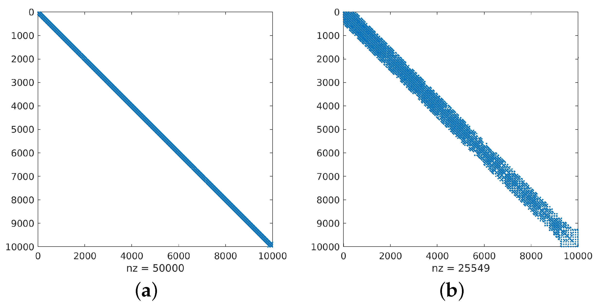
where $x_i$ is the coordinate vector of the pixel associated with the node $n_i$ and $h_{SGAF}=5$. The weighted adjacency matrix ${\mathit{A}}_{SGAF}$ of the graph ${\mathit{G}}_{SGAF}$ is defined as in Equation (40). The considered Laplacian matrix ${\mathit{L}}_{SGAF}$ is the Symmetric Normalized one as defined in Equation (45) (see Figure 11a for the sparsity representation of ${\mathit{L}}_{SGAF}$), and its condition number in L2 norm is $\kappa \left({\mathit{L}}_{SGAF}\right)=1.691915e+17$.

Example 2. 

A weighted graph ${\mathit{G}}_{SPGAF}$ is considered where the set $\mathit{N}$ of nodes coincides with the set of all the pixel values of $I_{toy}$. Two nodes $n_i,n_j\in \mathit{N}$ are considered connected by an edge if $n_i$ is among the 50 nearest neighbors of $n_j$ and $n_j$ is among the 50 nearest neighbors of $n_i$ in both of two distances: the Spatial Gaussian affinity function and the Photometric Gaussian affinity function [57]. The distance $w_{i,j}^{SPGAF}$ between connected nodes $n_i,n_j\in \mathit{N}$ is then defined as

$$w_{i,j}^{SPGAF}=exp\left(-{\displaystyle \frac{∥x_i-x_j∥}{h_{SGAF}^2}}\right)exp\left(-{\displaystyle \frac{∥z_i-z_j∥}{h_{PGAF}^2}}\right)$$

(57)

where $x_i$ is the coordinate vector of the pixel associated with the node $n_i$, $z_i$ is the grayscale value of the pixel associated with the node $n_i$, $h_{SGAF}=10$, and $h_{PGAF}=5$. The weighted adjacency matrix ${\mathit{A}}_{SPGAF}$ of the graph ${\mathit{G}}_{SPGAF}$ is defined as in Equation (40). The considered Laplacian matrix ${\mathit{L}}_{SPGAF}$ is based on Equation (43) (see Figure 11b for the sparsity representation of ${\mathit{L}}_{SPGAF}$), and its condition number in L2 norm $\kappa \left({\mathit{L}}_{SPGAF}\right)=$ is numerically infinite.

In both examples, no scaling operation is performed on the Laplacian matrix. Moreover, the HM representation of the Laplacian matrix considered is based on the following parameters: $ϵ=1\times {10}^{-08}$, $k=1$. The coefficients of the polynomial are generated randomly as a result of a uniform distribution in the interval $\left[0,1\right]$.

In

Table 3. Results from tests on GC-DNN toy examples.

Example 1
$n=6$
s	$E\left({\mathit{L}}_{SGAF},n,s\right)$	$E\left({\mathit{L}}_{SGAF}\mathbf{s}\right)$
3	$1.754\times {10}^{-15}$	$1.655\times {10}^{-11}$
4	$1.416\times {10}^{-15}$	$1.428\times {10}^{-11}$
5	$1.403\times {10}^{-15}$	$1.180\times {10}^{-11}$
$n=8$
s	$E\left({\mathit{L}}_{SGAF},n,s\right)$	$E\left({\mathit{L}}_{SGAF}\mathbf{s}\right)$
3	$1.987\times {10}^{-06}$	$8.051\times {10}^{-03}$
4	$1.987\times {10}^{-06}$	$8.057\times {10}^{-03}$
5	$1.987\times {10}^{-06}$	$8.051\times {10}^{-03}$
$n=10$
s	$E\left({\mathit{L}}_{SGAF},n,s\right)$	$E\left({\mathit{L}}_{SGAF}\mathbf{s}\right)$
3	$3.303\times {10}^{-05}$	$1.588\times {10}^{-02}$
4	$4.817\times {10}^{-06}$	$2.278\times {10}^{-03}$
5	$1.484\times {10}^{-04}$	$8.376\times {10}^{-01}$
Example 2
$n=6$
s	$E\left({\mathit{L}}_{SPGAF},n,s\right)$	$E\left({\mathit{L}}_{SGAF}\mathbf{s}\right)$
3	$4.795\times {10}^{-08}$	$1.347\times {10}^{-05}$
4	$4.747\times {10}^{-08}$	$1.368\times {10}^{-05}$
5	$6.289\times {10}^{-08}$	$1.411\times {10}^{-05}$
$n=8$
s	$E\left({\mathit{L}}_{SPGAF},n,s\right)$	$E\left({\mathit{L}}_{SGAF}\mathbf{s}\right)$
3	$1.517\times {10}^{-05}$	$3.148\times {10}^{-03}$
4	$2.091\times {10}^{-05}$	$3.831\times {10}^{-03}$
5	$1.776\times {10}^{-05}$	$3.144\times {10}^{-03}$
$n=10$
s	$E\left({\mathit{L}}_{SPGAF},n,s\right)$	$E\left({\mathit{L}}_{SGAF}\mathbf{s}\right)$
3	$5.320\times {10}^{-02}$	$9.671\times {10}^{+00}$
4	$5.686\times {10}^{-02}$	$1.109\times {10}^{+01}$
5	$7.158\times {10}^{-02}$	$1.179\times {10}^{+01}$

, the following are listed for different values of the polynomial degree n and different values s for the factors ${\mathit{B}}_k$ degree:

• the norm $E\left({\mathit{L}}_{SGAF},n,s\right)$, already defined in Section 3, of the difference between the results of the polynomial evaluation operations performed with and without an HM representation for matrices;
• the norm $E\left({\mathit{L}}_{SGAF}\mathbf{s}\right)$ of the difference between the results of the matrix–vector operations performed with and without HM-based algorithms.

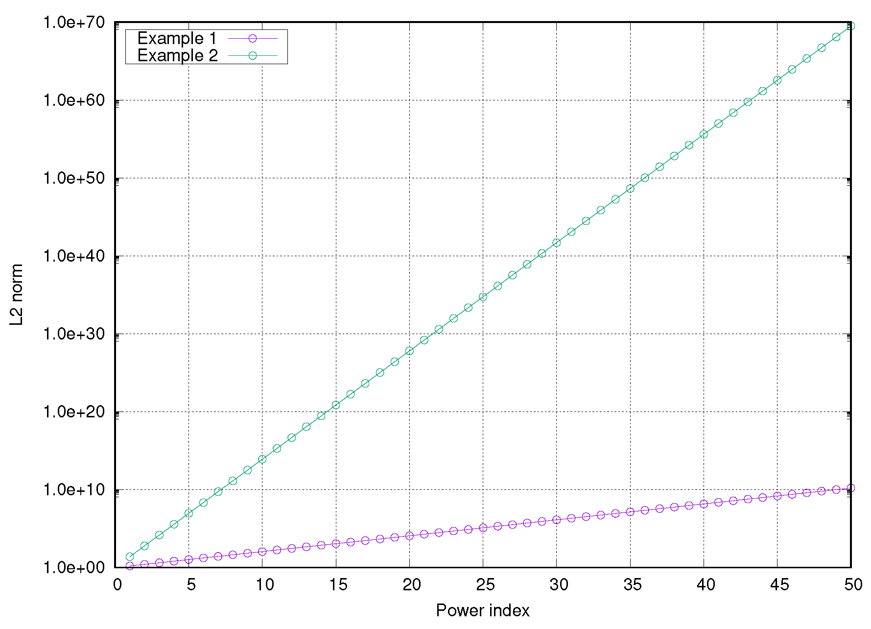
Looking at Table 3, the explosion of both the errors $E\left({\mathit{L}}_{SPGAF},n,s\right)$ and $E\left({\mathit{L}}_{SGAF}\mathbf{s}\right)$ attracts attention (especially for the second example). As suggested by Higham [58], the results of these preliminary tests confirm the problems related to the evaluation of matrix power, i.e., ${\mathit{M}}^n$. In particular, what makes the difference is not only the matrix condition number but also the behavior of the sequence $∥{\mathit{M}}^n∥,k=1,\dots n$. In Figure 12, we report the trends of the L2 norm of the Laplacian matrices’ powers $∥{\mathit{L}}_{*}^i∥$ for both the GC-DNN toy examples as functions of the power index i.

Therefore, while the possibility of using HM in the GC-DNN context remains an interesting option, much work remains to be conducted to (1) identify the matrix characteristics that make it less sensitive to error amplification or (2) to define mitigation strategies to reduce such amplification.

5. Conclusions and Future Work

Following a co-design approach that historically often guides and influences the evolution of the algorithms for the upcoming computing systems, this is the moment, at the dawn of the exascale Computing Era, to invest once again in the development of new algorithms that meet the growing need to ensure a high level of scalability and granularity.

In this context, methods based on hierarchical matrices (HMs) have been included among the most promising in the use of new computing resources precisely because of their strongly hierarchical nature.

This work aims to begin establishing the advantages and limitations of using HMs in operations such as the evaluation of matrix polynomials, which are crucial, for example, in the Graph Convolutional Deep Neural Network (GC-DNN) context. The presented tests show how the use of HMs still seems to be far from effective in complex contests such as matrix polynomial evaluation in real applications. These difficulties seem to be related to some characteristics of the matrices, such as their sparsity pattern or their max values [58].

So, bearing in mind the idea of building a truly effective and efficient tool that can make the most of modern supercomputing architectures, our future work will focus on the following: (1) a theoretical study of the characteristics of the matrices that make them more suitable (in terms of error propagation and memory occupancy) for an HM representation in the context of the evaluation of matrix polynomials; (2) the definition of a mitigation strategy for issues that lead to error amplification in order to achieve more stable algorithms [58]: techniques based on permutation, scaling, and/or normalization of the matrices could be considered; (3) the full implementation, in an HPC context, of the presented algorithms (i.e., see Algorithms 6 and 8) and the evaluation of their performances; (4) the validation of the proposed approach in a real application (i.e., from the strategic GC-DNN context).

Although the interest in hierarchical matrices is still high, even among those who develop mathematical software libraries (see for example the list available in [59]), and despite the high potential announced in works that, a decade ago, imagined the future for supercomputing [25], the current investment in the creation of parallel software libraries based on hierarchical matrices and their use seems very poor (one can mention the HMLib library [60] or the experiments from MAGMA developers [61,62]). We, therefore, hope that this work can be a stimulus in reviving interest in such tools in advanced computing contexts.

References

1. Higham, N. Functions of Matrices: Theory and Computation; Other Titles in Applied Mathematics, Society for Industrial and Applied Mathematics (SIAM): Philadelphia, PA, USA, 2008. [Google Scholar]
2. Wang, B.; Kestelyn, X.; Kharazian, E.; Grolet, A. Application of Normal Form Theory to Power Systems: A Proof of Concept of a Novel Structure-Preserving Approach. In Proceedings of the 2024 IEEE Power & Energy Society General Meeting (PESGM), Seattle, WA, USA, 21–25 July 2024; pp. 1–5. [Google Scholar] [CrossRef]
3. Schmelzer, T.; Trefethen, L.N. Evaluating matrix functions for exponential integrators via Carathéodory-Fejér approximation and contour integrals. Electron. Trans. Numer. Anal. 2007, 29, 1–18. [Google Scholar]
4. Daigavane, A.; Ravindran, B.; Aggarwal, G. Understanding Convolutions on Graphs. Distill 2021. [Google Scholar] [CrossRef]
5. Defferrard, M.; Bresson, X.; Vandergheynst, P. Convolutional neural networks on graphs with fast localized spectral filtering. In Proceedings of the 30th International Conference on Neural Information Processing Systems, Barcelona, Spain, 5–10 December 2016; pp. 3844–3852. [Google Scholar]
6. Carracciuolo, L.; Lapegna, M. Implementation of a non-linear solver on heterogeneous architectures. Concurr. Comput. Pract. Exp. 2018, 30, e4903. [Google Scholar] [CrossRef]
7. Mele, V.; Constantinescu, E.M.; Carracciuolo, L.; D’Amore, L. A PETSc parallel-in-time solver based on MGRIT algorithm. Concurr. Comput. Pract. Exp. 2018, 30, e4928. [Google Scholar] [CrossRef]
8. Carracciuolo, L.; Mele, V.; Szustak, L. About the granularity portability of block-based Krylov methods in heterogeneous computing environments. Concurr. Comput. Pract. Exp. 2021, 33, e6008. [Google Scholar] [CrossRef]
9. Carracciuolo, L.; Casaburi, D.; D’Amore, L.; D’Avino, G.; Maffettone, P.; Murli, A. Computational simulations of 3D large-scale time-dependent viscoelastic flows in high performance computing environment. J.-Non-Newton. Fluid Mech. 2011, 166, 1382–1395. [Google Scholar] [CrossRef]
10. Carracciuolo, L.; D’Amore, L.; Murli, A. Towards a parallel component for imaging in PETSc programming environment: A case study in 3-D echocardiography. Parallel Comput. 2006, 32, 67–83. [Google Scholar] [CrossRef]
11. Murli, A.; D’Amore, L.; Carracciuolo, L.; Ceccarelli, M.; Antonelli, L. High performance edge-preserving regularization in 3D SPECT imaging. Parallel Comput. 2008, 34, 115–132. [Google Scholar] [CrossRef]
12. D’Amore, L.; Constantinescu, E.; Carracciuolo, L. A Scalable Space-Time Domain Decomposition Approach for Solving Large Scale Nonlinear Regularized Inverse Ill Posed Problems in 4D Variational Data Assimilation. J. Sci. Comput. 2022, 91. [Google Scholar] [CrossRef]
13. Carracciuolo, L.; D’Amora, U. Mathematical Tools for Simulation of 3D Bioprinting Processes on High-Performance Computing Resources: The State of the Art. Appl. Sci. 2024, 14, 6110. [Google Scholar] [CrossRef]
14. Reed, D.A.; Dongarra, J. Exascale Computing and Big Data. Commun. ACM 2015, 58, 56–68. [Google Scholar] [CrossRef]
15. Petitet, A.; Whaley, R.C.; Dongarra, J.; Cleary, A. A Portable Implementation of the High-Performance Linpack Benchmark for Distributed-Memory Computers. Innovative Computing Laboratory. 2000. Available online: https://icl.utk.edu/hpl/index.html (accessed on 1 April 2025).
16. Top 500—The List. Available online: https://www.top500.org/ (accessed on 1 April 2025).
17. Top 500 List—June 2022. Available online: https://www.top500.org/lists/top500/2022/06/ (accessed on 1 April 2025).
18. Geist, A.; Lucas, R. Major Computer Science Challenges At Exascale. Int. J. High Perform. Comput. Appl. 2009, 23, 427–436. [Google Scholar] [CrossRef]
19. Chen, W. The demands and challenges of exascale computing: An interview with Zuoning Chen. Natl. Sci. Rev. 2016, 3, 64–67. [Google Scholar] [CrossRef]
20. Kumar, V.; Gupta, A. Analyzing Scalability of Parallel Algorithms and Architectures. J. Parallel Distrib. Comput. 1994, 22, 379–391. [Google Scholar] [CrossRef]
21. Kwiatkowski, J. Evaluation of Parallel Programs by Measurement of Its Granularity. In Proceedings of the Parallel Processing and Applied Mathematics; Wyrzykowski, R., Dongarra, J., Paprzycki, M., Waśniewski, J., Eds.; Springer: Berlin/Heidelberg, Germany, 2002; pp. 145–153. [Google Scholar] [CrossRef]
22. Ewart, T.; Cremonesi, F.; Schürmann, F.; Delalondre, F. Polynomial Evaluation on Superscalar Architecture, Applied to the Elementary Function ex. ACM Trans. Math. Softw. 2020, 46, 28. [Google Scholar] [CrossRef]
23. Munro, I.; Paterson, M. Optimal algorithms for parallel polynomial evaluation. In Proceedings of the 12th Annual Symposium on Switching and Automata Theory (SWAT 1971), East Lansing, MI, USA, 13–15 October 1971; pp. 132–139. [Google Scholar] [CrossRef]
24. Keyes, D.E. Exaflop/s: The why and the how. Comptes Rendus. MÉcanique 2011, 339, 70–77. [Google Scholar] [CrossRef]
25. Ang, J.; Evans, K.; Geist, A.; Heroux, M.; Hovland, P.D.; Marques, O.; Curfman McInnes, L.; Ng, E.G.; Wild, S.M. Report on the Workshop on Extreme-Scale Solvers: Transition to Future Architectures. Report, U.S. Department of Energy, ASCR, 2012. Available online: https://science.osti.gov/-/media/ascr/pdf/program-documents/docs/reportExtremeScaleSolvers2012.pdf (accessed on 1 April 2025).
26. Greengard, L.; Rokhlin, V. A fast algorithm for particle simulations. J. Comput. Phys. 1987, 73, 325–348. [Google Scholar] [CrossRef]
27. Martinsson, P.G. Fast Multipole Methods. In Encyclopedia of Applied and Computational Mathematics; Springer: Berlin/Heidelberg, Germany, 2015; pp. 498–508. [Google Scholar] [CrossRef]
28. Cipra, B.A. The Best of the 20th Century: Editors Name Top 10 Algorithms. SIAM News 2000, 33, 1–2. [Google Scholar]
29. Beatson, R.; Greengard, L. A Short Course on Fast Multipole Methods, 2001. Available online: https://math.nyu.edu/~greengar/shortcourse_fmm.pdf (accessed on 1 April 2025).
30. Fenn, M.; Steidl, G. FMM and H-Matrices: A Short Introduction to the Basic Idea. Technical Report, Department for Mathematics and Computer Science, University of Mannheim, 2002. Available online: https://madoc.bib.uni-mannheim.de/744/ (accessed on 1 April 2025).
31. Hackbusch, W.; Grasedyck, L.; Börm, S. An introduction to hierarchical matrices. Math. Bohem. 2002, 127, 229–241. [Google Scholar] [CrossRef]
32. Hackbusch, W. Hierarchical Matrices: Algorithms and Analysis, 1st ed.; Springer Series in Computational Mathematics; Springer: Berlin/Heidelberg, Germany, 2015. [Google Scholar] [CrossRef]
33. Borm, S.; Grasedyck, L.; Hackbusch, W. Hierarchical Matrices. Technical Report, Max-Planck-Institut für Mathematik, 2003. Report Number: Lecture Notes 21/2003. Available online: https://www.mis.mpg.de/publications/preprint-repository/lecture_note/2003/issue-21 (accessed on 1 April 2025).
34. Yokota, R.; Turkiyyah, G.; Keyes, D. Communication Complexity of the Fast Multipole Method and its Algebraic Variants. Supercomput. Front. Innov. 2014, 1, 63–84. [Google Scholar] [CrossRef]
35. Saperas-Riera, J.; Mateu-Figueras, G.; Martín-Fernández, J.A. Lasso regression method for a compositional covariate regularised by the norm L1 pairwise logratio. J. Geochem. Explor. 2023, 255, 107327. [Google Scholar] [CrossRef]
36. Serajian, M.; Marini, S.; Alanko, J.N.; Noyes, N.R.; Prosperi, M.; Boucher, C. Scalable de novo classification of antibiotic resistance of Mycobacterium tuberculosis. Bioinformatics 2024, 40, i39–i47. [Google Scholar] [CrossRef] [PubMed]
37. Lim, H. Low-rank learning for feature selection in multi-label classification. Pattern Recognit. Lett. 2023, 172, 106–112. [Google Scholar] [CrossRef]
38. Golub, G.H.; Van Loan, C.F. Matrix Computations, 3rd ed.; The Johns Hopkins University Press: Baltimore, ML, USA, 1996. [Google Scholar]
39. Weisstein, E.W. Binary Tree. From MathWorld—A Wolfram Web Resource, 2024. Available online: https://mathworld.wolfram.com/BinaryTree.html (accessed on 1 April 2025).
40. Grasedyck, L.; Hackbusch, W. Construction and Arithmetics of H-Matrices. Computing 2003, 70, 295–334. [Google Scholar] [CrossRef]
41. Graphical Representation of Sparse Matrices. Available online: https://www.mathworks.com/help/matlab/math/graphical-representation-of-sparse-matrices.html (accessed on 1 April 2025).
42. E20R5000: Driven Cavity, 20×20 Elements, Re = 5000. Available online: https://math.nist.gov/MatrixMarket/data/SPARSKIT/drivcav/e20r5000.html (accessed on 1 April 2025).
43. BCSSTK24: BCS Structural Engineering Matrices (Eigenvalue Problems) Calgary Olympic Saddledome Arena. Available online: https://math.nist.gov/MatrixMarket/data/Harwell-Boeing/bcsstruc3/bcsstk24.html (accessed on 1 April 2025).
44. The OpenMP API Specification for Parallel Programming. Available online: https://www.openmp.org/specifications/ (accessed on 1 April 2025).
45. Lawson, C.L.; Hanson, R.J.; Kincaid, D.R.; Krogh, F.T. Basic Linear Algebra Subprograms for Fortran Usage. ACM Trans. Math. Softw. 1979, 5, 308–323. [Google Scholar] [CrossRef]
46. BLAS and Sparse BLAS Routines of the Intel Math Kernel Library. Available online: https://www.intel.com/content/www/us/en/docs/onemkl/developer-reference-c/2024-1/blas-and-sparse-blas-routines.html (accessed on 1 April 2025).
47. Basic Linear Algebra on NVIDIA GPUs. Available online: https://developer.nvidia.com/cublas (accessed on 1 April 2025).
48. Paterson, M.S.; Stockmeyer, L.J. On the Number of Nonscalar Multiplications Necessary to Evaluate Polynomials. SIAM J. Comput. 1973, 2, 60–66. [Google Scholar] [CrossRef]
49. LeCun, Y.; Bengio, Y.; Hinton, G. Deep Learning. Nature 2015, 521, 436–444. [Google Scholar] [CrossRef]
50. Zhang, S.; Tong, H.; Xu, J.; Maciejewski, R. Graph convolutional networks: A comprehensive review. Comput. Soc. Netw. 2019, 6, 11. [Google Scholar] [CrossRef]
51. von Luxburg, U. A tutorial on spectral clustering. Stat. Comput. 2007, 17, 395–416. [Google Scholar] [CrossRef]
52. Chen, X. Understanding Spectral Graph Neural Network. arXiv 2020, arXiv:2012.06660. [Google Scholar]
53. Nikolaos, K. Spectral Graph Theory and Deep Learning on Graphs. Master’s Thesis, Department of Informatics, Aristotle University of Thessaloniki, Thessaloniki, Greece, 2017. [Google Scholar] [CrossRef]
54. Sandryhaila, A.; Moura, J.M.F. Discrete Signal Processing on Graphs. IEEE Trans. Signal Process. 2013, 61, 1644–1656. [Google Scholar] [CrossRef]
55. Sandryhaila, A.; Moura, J.M.F. Discrete signal processing on graphs: Graph fourier transform. In Proceedings of the 2013 IEEE International Conference on Acoustics, Speech and Signal Processing, Vancouver, BC, Canada, 26–31 May 2013; pp. 6167–6170. [Google Scholar] [CrossRef]
56. Shuman, D.I.; Narang, S.K.; Frossard, P.; Ortega, A.; Vandergheynst, P. The emerging field of signal processing on graphs: Extending high-dimensional data analysis to networks and other irregular domains. IEEE Signal Process. Mag. 2013, 30, 83–98. [Google Scholar] [CrossRef]
57. Wobrock, D. Image Processing Using Graph Laplacian Operator. Master’s Thesis, School of Electrical Engineering and Computer Science, KTH Royal Institute of Technology, Stockholm, Sweden, 2019. Available online: https://github.com/David-Wobrock/master-thesis-writing/blob/master/master_thesis_david_wobrock.pdf (accessed on 1 April 2025).
58. Higham, N.J. Accuracy and Stability of Numerical Algorithms, 2nd ed.; Society for Industrial and Applied Mathematics: Philadelphia, PA, USA, 2002. [Google Scholar]
59. Curated List of Hierarchical Matrices. Available online: https://github.com/gchavez2/awesome_hierarchical_matrices (accessed on 1 April 2025).
60. HLIBpro: Is a Software Library Implementing Algorithms for Hierarchical Matrices. Available online: https://www.hlibpro.com/ (accessed on 1 April 2025).
61. The Matrix Algebra on GPU and Multicore Architecture (MAGMA) Library Website. Available online: http://icl.cs.utk.edu/magma/ (accessed on 1 April 2025).
62. Yamazaki, I.; Abdelfattah, A.; Ida, A.; Ohshima, S.; Tomov, S.; Yokota, R.; Dongarra, J. Analyzing Performance of BiCGStab with Hierarchical Matrix on GPU Clusters. In Proceedings of the IEEE International Parallel and Distributed Processing Symposium (IPDPS), Vancouver, BC, Canada, 1 May 2018; Available online: https://icl.utk.edu/files/publications/2018/icl-utk-1049-2018.pdf (accessed on 1 April 2025).
Figure 1. The hierarchical architecture of modern HPC systems. Several processing units (core/CPU) are aggregated in a CPU/node and share some memory devices. Access to remote memory devices on other nodes is performed due to an interconnection network. Memory is organized into levels where access speed is inversely proportional to memory size and directly proportional to the memory distance from the processing units. Accelerators are a very particular type of processing unit with thousands of cores. Credit: Carracciuolo et al. [13].
Mathematics 13 01378 g001
Figure 8. Example of the execution tree of Algorithm 6. (a) Block structure of the H -matrix A . (b) Execution tree of Algorithm 6: (b.1) execution on the 1-st subtree; (b.2) execution on the 3-rd subtree; (b.3) execution on the 4-th subtree.
Mathematics 13 01378 g008
Figure 9. Example of parallel implementation of Algorithm 7 (and then of Algorithm 8) by using N T a s k s = 4 and r = 7 .
Mathematics 13 01378 g009
Figure 10. An image for GC-DNN toy examples.
Mathematics 13 01378 g010
Figure 11. Sparsity representation of the Laplacian matrices for GC-DNN toy examples. (a) Example 1. (b) Example 2.
Mathematics 13 01378 g011
Figure 12. Trends, as function of the power index i, of the L2 norm of the Laplacian matrices’ powers L * i for both the GC-DNN toy examples.
Mathematics 13 01378 g012