Abstract
Deep neural networks (DNNs) have achieved high accuracy in various applications, but with the rapid growth of AI and the increasing scale and complexity of datasets, their computational cost and power consumption have become even more significant challenges. Spiking neural networks (SNNs), inspired by biological neurons, offer an energy-efficient alternative by using spike-based information processing. However, training SNNs is difficult due to the non-differentiability of their activation function and the challenges in constructing deep architectures. This study addresses these issues by integrating DNN-like backpropagation into SNNs using a supervised learning approach. A surrogate gradient descent based on the arctangent function is applied to approximate the non-differentiable activation function, enabling stable gradient-based learning. The study also explores the interplay between the spatial domain (layer-wise propagation) and the temporal domain (time step), ensuring proper gradient propagation using the chain rule. Additionally, mini-batch training, Adam optimization, and layer normalization are incorporated to improve training efficiency and mitigate gradient vanishing. A softmax-based probability representation and cross-entropy loss function are used to optimize classification performance. Along with these techniques, a deep SNN was designed to converge to the optimal point faster than other models in the early stages of training by utilizing a modified learning rate scheduler. The proposed learning method allows deep SNNs to achieve competitive accuracy while maintaining their inherent low-power characteristics. These findings contribute to making SNNs more practical for machine learning applications by combining the advantages of deep learning and biologically inspired computing. In summary, this study contributes to the field by analyzing and adapting deep learning techniques—such as dropout, layer normalization, mini-batch training, and Adam optimization—to the spiking domain, and by proposing a novel learning rate scheduler that enables faster convergence during early training phases with fewer epochs.
Keywords:
spiking neural networks; deep learning; learning rate scheduler; gradient descent; neuromorphic MSC:
68T07; 68Q32
1. Introduction
Deep neural networks (DNNs) have achieved remarkable success in various fields. With the continuous advancement of artificial intelligence, the importance of deep learning has been further reinforced. However, the high computational cost associated with training DNNs raises significant concerns regarding power efficiency [1,2,3,4,5,6].
To address this issue, a new generation of neural networks, namely spiking neural networks (SNNs), has emerged. SNNs are inspired by the human brain and closely mimic biological neural processes, enabling high performance with significantly lower power consumption [7,8]. This is primarily due to their information transmission mechanism, which utilizes spikes instead of continuous values. Unlike DNNs, where forward propagation involves real-valued computations, SNNs transmit information using binary spikes (0 or 1).
Despite their advantages, training SNNs presents significant challenges. The activation function of neurons in SNNs most commonly uses the LIF model [9,10,11], which has a form similar to that of the Dirac delta function. Consequently, these neurons produce discrete spike-shaped outputs, making them inherently non-differentiable. As a result, conventional backpropagation-based training methods used in DNNs cannot be directly applied to SNNs. Instead, SNNs are often trained using unsupervised learning techniques that leverage timing-based parameters. A well-known example is spike-timing-dependent plasticity (STDP), which updates synaptic weights based on the relative timing of spikes between pre- and post-synaptic neurons. However, this approach has limitations, particularly in training deep networks with multiple hidden layers [12], leading to lower predictive accuracy.
To overcome these challenges, this study introduces a supervised learning approach for training SNNs that is inspired by the backpropagation mechanism used in DNNs. Specifically, the proposed method applies gradient descent to optimize network parameters in a supervised manner, enabling the construction of deep SNN architectures. However, as mentioned earlier, the delta Dirac activation function in SNNs is non-differentiable, making direct gradient-based optimization infeasible. To address this issue, we employ the surrogate gradient descent, which approximates the non-differentiable activation function with a differentiable alternative during gradient descent.
In this study, we not only adopt the training framework of DNNs but also explore how SNNs process information in the temporal domain [13,14] and how the chain rule can be simplified to facilitate gradient-based learning. Furthermore, a novel modified learning rate scheduler technique is proposed to enable faster convergence to the optimal point in the early training phase compared to other models, along with the most effective techniques for such SNNs. A deep SNN incorporating all these techniques is compared with a conventional DNN to validate the performance of the proposed DSNN.
The remainder of this paper is structured as follows. Section 2 provides a detailed explanation of the network composition, including the SNN neuron model, spike activity, network architecture, loss function, and learning model, along with the proposed modified learning rate scheduler and the overall algorithm. Section 3 presents a performance evaluation by comparing the proposed deep SNN with other models. Section 4 provides a detailed discussion of the underlying reasons for the DSNN’s superior performance, including its temporal dynamics and the effects of the learning rate scheduler. Finally, Section 5 concludes the paper with a summary of the findings, implications, and future research directions.
2. Materials and Methods
2.1. Neuron Model
In the proposed deep SNN model, the activation function of each neuron is based on the Leaky Integrate-and-Fire (LIF) model. In LIF, the membrane potential at the current time step is determined by the weighted sum of inputs and the membrane potential from the previous time step. The membrane potential accumulates over time, and, when it exceeds a predefined membrane threshold, the neuron fires. Upon firing, the neuron generates a spike, which takes a value of 1. If the neuron does not fire, the output remains 0.
To formalize the LIF neuron, several key components are required [8]. First, the spike values from the previous neurons and the synaptic weights connecting the two neurons play a crucial role. The weighted sum of the spikes from all previous neurons connected to the current neuron forms an essential term in the computation. Mathematically, this can be represented in matrix form, as follows:
where is the weight matrix representing the synapses connecting layer to layer l and is the vector of spikes from layer at time step .
In the LIF neuron model of SNNs, the membrane potential gradually decreases over time. This phenomenon is referred to as the leak of the membrane potential. This characteristic can be represented in the membrane potential term at the current time step t, as shown in Equation (2). Here, leak factor is a constant within the range of 0 to 1, representing the leaky nature of the LIF model. This constant modulates the leakage effect of the membrane potential. The matrix represents the membrane potential in time step t in layer l. The process of how the membrane potential evolves over time can be observed in Figure 1.
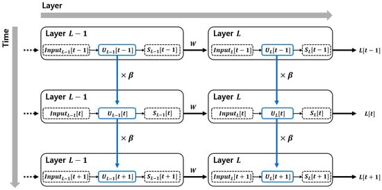
Figure 1.
Backpropagation through time (BPTT) in spiking neural networks. The temporal dependencies of the membrane potential are propagated across time steps. Blue arrows represent the temporal influence of membrane potential modulated by the leak factor , indicating how previous membrane states affect the current potential. Gray arrows indicate the direction of information flow: horizontal arrows represent the progression over time, while vertical arrows represent feedforward propagation across layers.
The membrane potential at the current time step is influenced by the values from previous time steps. In other words, it is continuously affected by the membrane potential from earlier moments in time. This reveals that spiking neural networks (SNNs) operate not only in the spatial domain but also in the temporal domain, which is reflected through the behavior of the membrane potential.
When a neuron’s membrane potential exceeds the membrane threshold, the neuron fires and its membrane potential is reset. The firing frequency of the neuron can be controlled using the membrane threshold and the reset scaling factor. If the goal is to promote sparse spiking for high energy efficiency in hardware implementation, the membrane threshold can be set relatively high to suppress frequent firing. During the reset phase, the membrane potential is typically reduced by subtracting the membrane threshold value, bringing it close to its initial state. However, this reset behavior can also be adjusted by applying a scaling factor (as shown in Equation (3)) to the membrane threshold, thereby controlling how much the potential is reset. When the reset scaling factor is applied, the membrane potential is reset to a higher value compared to when the scaling factor is not used. As a result, the neuron can fire again after a shorter duration. This mechanism can be used to increase the amount of information carried by generating more spikes, which in turn may lead to more accurate results.
The reset scaling factor and the membrane threshold are defined as follows:
By incorporating all terms that influence the membrane potential of the neurons [8], the overall update equation can be expressed as follows:
where represents the membrane potential vector of neurons in layer l at time step .
2.2. Spike Activity
In the LIF neuron model of an SNN, the membrane potential is checked at each time step to determine whether it exceeds the membrane threshold. If the membrane potential exceeds the threshold, the neuron outputs a value of 1; otherwise, it outputs 0. In other words, each neuron produces an output in the form of a spike, which is either 0 or 1. This follows the form of a Dirac delta function and can be mathematically expressed as follows:
While this activation function does not pose any issues during the forward pass, it becomes problematic in the backward pass due to its non-differentiability. Consequently, this function cannot be directly utilized in the backpropagation process. Instead, a surrogate gradient descent is employed [15], wherein the non-differentiable function is replaced with a differentiable approximation.
To apply surrogate gradient descent, several differentiable activation functions have been proposed to replace the original non-differentiable activation function. A common approach is to approximate the Dirac delta function using activation functions such as sigmoid or ReLU, which are frequently used in DNNs. However, these functions can suffer from gradient vanishing issues when applied to deep learning-based SNNs, making them impractical for effective training.
To address this, we employ an experimentally validated surrogate gradient descent based on the arctangent function [16]. The arctangent function is differentiable, allowing for smooth gradient computation during training. The surrogate gradient descent formulation is expressed as follows:
In the above equation, is the derivative scaling factor, which is typically set to 2.
The derivative of spike activity with respect to the membrane potential is given by the following equation:
By adopting this surrogate gradient descent, the original non-differentiable activation function is replaced with a differentiable function during the backpropagation process. This replacement enables the computation of gradients during backpropagation, allowing the training process to be properly carried out.
2.3. Network Architecture
The spiking neural network (SNN) consists of an input layer, multiple hidden layers, and an output layer. The neurons in the input layer receive input data and transmit spikes to the next layer. In the hidden layers, neurons process incoming spike activities and relay information to the next layers. The final output layer computes the network’s final output, which is then used to calculate the loss at the output neurons. However, training an SNN effectively through such a conventional network structure presents challenges.
When training with deep learning methods, the number of parameters increases exponentially as the number of layers grows. This leads to excessive memory consumption and significant computational overhead, which undermines the efficiency of SNNs, especially considering their primary advantage of low power consumption. To address this issue, in this study, the mini-batch gradient descent [17] was utilized. In the case of mini-batch processing, parameters are not updated for each individual data point; instead, they are updated only once for a batch of data, enabling efficient computation. Moreover, when implementing the model in hardware, computations can be performed in parallel for an entire batch at once, which is another reason for adopting the mini-batch gradient descent approach.
Furthermore, mini-batch training benefits from the Adam optimizer [18], which combines the advantages of momentum and RMSprop to enhance optimization performance. The Adam optimizer calculates moment vectors to adjust the direction and magnitude of parameter updates efficiently. This helps mitigate the problem of getting trapped in local minima, which is a common limitation in deep learning. Moreover, as SNNs transmit information through spikes, they are inherently prone to gradient vanishing issues. The Adam optimizer alleviates this problem by ensuring stable gradient flow during training.
However, the SNN architecture, which incorporates temporal dependencies, introduces additional challenges. When input data enters the network across multiple time steps, rate-encoding methods can cause each time step’s input pixels to exhibit similar patterns. This can lead to certain neurons continuously generating spikes while others rarely fire, eventually resulting in some neurons never spiking. Such neurons, often referred to as dead neurons, become ineffective in the network. To mitigate this issue, a dropout mechanism [19] is applied.
Dropout prevents specific neurons from firing spikes by randomly deactivating a subset of neurons in each layer during training. This ensures that certain neurons do not dominate spike activity, thereby preventing specific synapses from being overly trained. The dropout technique is implemented using a dropout mask, which randomly deactivates neurons, promoting balanced learning across all neurons in the hidden layers.
Since SNNs rely on spike-based information transmission, neuron activation values can become unevenly distributed, leading to difficulties in learning. To address this, layer normalization is applied to each hidden layer, ensuring that layer outputs remain within a controlled range, thereby stabilizing the learning process. Unlike batch normalization, which depends on batch size, layer normalization normalizes the activation values of individual neurons independently of batch size. This flexibility allows it to be easily applied regardless of batch size variations.
By implementing these strategies, we optimize the training process for SNNs, improving computational efficiency, memory utilization, and training stability.
2.4. Loss Function
In spiking neural networks (SNNs), the network must be trained to generate more spikes for the correct label. During training, it is essential to monitor the activation level of the neuron corresponding to the correct label. There are two primary indicators of neuronal activation: membrane potential and spike count. Membrane potential provides the most direct representation of a neuron’s activation level, while spike count conveys the overall activation level by counting the number of spikes each neuron generates over the entire time step.
The loss is calculated after the completion of forward propagation; that is, when all time steps have been processed. During this process, the membrane potential generates multiple spikes and is reset several times. As a result, at the final time step, when the loss is evaluated, the membrane potential may have been reset and may appear to show no activation at all. However, in the case of the spike count, the spikes are accumulated throughout all time steps without being reset. Therefore, when measuring the loss in an SNN, it is more accurate to evaluate the activation level of each neuron based on its total spike count.
Therefore, the probability of each output neuron is calculated based on the spike count, and this value is then used in the loss function. In this study, we adopt the cross-entropy loss function [20], which is widely used for multi-class classification in supervised learning. In a network that classifies data with multiple classes, the loss for each neuron in the output layer is calculated by comparing the activation level of each neuron with the target label. Based on these loss values, gradient descent is performed to train the parameters of the network. After repeatedly training the network using these loss values, the neurons in the output layer of the trained network are guided to fire more spikes for the correct label. As a result, once training is sufficiently completed, the neurons in the output layer produce more spikes corresponding to the correct label.
To implement this, the spike count is input into the softmax function [21] to obtain the probability of each output neuron. Then, these probability values are fed into the cross-entropy loss function to compute the loss for each output neuron. In the following softmax equation, represents the value of the ith output neuron at time step t, and denotes the total accumulated spike count of the ith output neuron at time step t. Furthermore, C represents the number of correct labels.
Using the softmax function, the cross-entropy loss is formulated as follows:
where represents the one-hot encoded label corresponding to the correct class.
2.5. Learning Model
In deep neural networks (DNNs), learning is conducted through backpropagation, where gradient descent is used to compute gradients and update parameters. While DNNs achieve high accuracy, their real-valued outputs demand extensive computational resources. In contrast, SNNs utilize spike-based outputs, which take binary values (0 or 1). SNNs have significantly simpler values for each term during the gradient descent process than DNNs, allowing for lower computational complexity in the backpropagation process.
Traditional SNN learning methods rely solely on the temporal domain, where learning occurs through spike-timing-dependent plasticity (STDP), based on the spike times of pre- and post-synaptic neurons. However, this approach makes it challenging to train deep networks with multiple hidden layers, ultimately limiting their ability to learn complex datasets. Although SNNs offer lower power consumption than DNNs, their accuracy deteriorates when handling intricate tasks.
To address these limitations, this study integrates the advantages of DNNs into SNN learning by adopting backpropagation with gradient descent. In SNNs, both the temporal domain and the spatial domain coexist [13]. The temporal domain represents the sequential evolution of membrane potentials across time steps, while the spatial domain corresponds to the hierarchical structure of multiple hidden layers. For effective propagation across these domains, certain structural connections within the SNN network must be considered.
In the spatial domain, each layer is connected through synaptic weights. However, the connections in the temporal domain are implicit. This can be observed in the membrane potential equation, where the first term involves a leaky constant multiplying the membrane potential from the previous time step. This illustrates the inherent temporal connectivity of SNNs. Using this relationship, the chain rule can be effectively applied to the backpropagation process.
2.5.1. Gradient Computation via Chain Rule
During backpropagation, gradient descent is applied using the chain rule. To construct the chain rule, we must trace the loss function back through the network, starting from the output and propagating backward. This process is expressed in Figure 2.
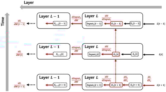
Figure 2.
Backpropagation over time in spiking neural networks. The figure illustrates the gradient flow in the temporal domain, where the membrane potential propagates across time steps, and the gradient of the loss function is computed using the chain rule. Red arrows indicate the flow of partial derivatives during backpropagation, showing how each term in the chain rule contributes to the gradient computation. Horizontal arrows represent the backward gradient propagation across layers, while vertical arrows indicate the backward gradient flow across time steps.
First, to compute the parameter update, the gradient must be derived from the loss function. Since the loss function is expressed in terms of spike-based outputs in a matrix form, the first term in the chain rule is given by the following equation.
where represents the softmax probability matrix, as follows:
By differentiating the probability matrix with respect to the accumulated spike count , we obtain the following:
From the definition of accumulated spike count, the differentiation with respect to spike activity is as follows:
Thus, combining these terms, the gradient can be expressed as follows:
Simplifying this equation, we obtain the following:
which is finally expressed as follows:
where represents the target probability matrix for classification.
After computing the gradient with respect to spike activity, we now consider the membrane potential. As discussed in Section 2, the Dirac delta function is non-differentiable, requiring the use of a surrogate gradient descent for backpropagation. Here, we approximate the activation function using the arctangent function in a matrix form, whose derivative is as follows:
This approximation ensures smooth gradient propagation while maintaining the spiking nature of SNNs.
To account for the influence of previous time steps, the membrane potential must be differentiated with respect to its earlier states. As described in the temporal domain formulation, the recurrence relation in membrane potential is given in matrix form as follows:
Thus, differentiating with respect to the previous time step, we obtain the following:
Next, we consider the dependency on input activity. The membrane potential equation shows that one of its terms corresponds to input activity, implying the following:
Since input activity is the product of synaptic weight and spike activity, differentiating with respect to the synaptic weights gives the following:
Similarly, differentiating with respect to the spike activity at the previous layer results in the following equation:
2.5.2. Extending to Deep SNN Architectures
The above process applies to networks with a single hidden layer. However, for deeper networks, multiple hidden layers must be incorporated. To compute the gradients efficiently, the chain rule must be reused across layers. When multiple hidden layers are present, the backward pass follows a similar structure.
For networks with two hidden layers, the gradient propagation follows the same recursive structure, ensuring computational efficiency. This allows the reuse of previously computed gradients to optimize memory and computational efficiency. Ultimately, this approach facilitates deep SNN training while preserving biological plausibility and energy efficiency.
2.6. Modified Learning Rate Scheduler
The ADAM optimizer [18] adaptively adjusts each parameter by leveraging the first and second moments of the gradient, inherently modifying the learning rate within the optimizer. Therefore, at first glance, using the ADAM optimizer may seem to eliminate the need for a learning rate scheduler. However, there are still aspects of the ADAM optimizer that can be improved. The most crucial aspect of a neural network is how quickly and accurately it learns. To accelerate learning, the early epochs, where most of the learning takes place, should involve the most significant updates. In other words, the learning rate should be adjusted sharply during the initial epochs to maximize the learning impact. To adjust the learning rate, the Adam optimizer should be used while additionally applying a learning rate scheduler.
There are various types of learning rate schedulers. In this study, we empirically verified various learning rates to identify the most suitable one for the given network. By experimenting with different learning rate schedulers, including lambda, exponential [22], multiplicative, and cosine annealing [23], we found that the lambda learning rate scheduler achieved the best performance for this network.
However, while using only a learning rate scheduler enables stable training, there were few differences in the early epochs compared to using the standard ADAM optimizer alone. Therefore, to achieve faster convergence in the early epochs, the existing learning rate scheduler was modified.
First, the gradient of the loss was calculated based on the difference between the recent loss and the loss from the previous batch. The cases were then divided based on whether this gradient was positive or negative. If the gradient was positive, it indicated an increase in loss, likely due to an excessively large learning rate causing oscillations. In this case, the learning rate was decreased accordingly.
When the gradient was negative, three different cases were considered. The degree of the negative gradient was categorized into three levels. Since it is desirable to have a steep gradient during the early epochs for rapid learning, different adjustments were applied based on the steepness of the gradient. If the gradient was in the steepest range, the learning rate was maintained. If the gradient was in the second steepest range, the learning rate was slightly increased to encourage movement toward the steepest gradient range. Finally, if the gradient was in the lowest range, the learning rate was significantly increased to accelerate convergence toward the optimal steep region.
The following equation adjusts the learning rate when the loss is decreasing, adapting it based on the gradient magnitude in three cases. Here, is the learning rate scaling factor, which scales the learning rate in the modified learning rate scheduler, and is the additional scaling factor, which applies further adjustments beyond the second stage.
2.7. Algorithm
The complete training algorithm, including both the forward pass and backward pass when using two hidden layers, is set out in Algorithm 1 below.
| Algorithm 1 Training algorithm for spiking neural network with modified learning rate scheduler. |
Require: Training data , test data
|
3. Results
To evaluate the performance of the deep SNN, we compared it with a conventional DNN using the same environment and network techniques. In the DNN, we employed the same mini-batch, dropout, layer normalization, and Adam optimizer used in the deep SNN. The activation function was set to ReLU, and the same loss function was applied. The dataset used was the Modified National Institute of Standards and Technology (MNIST) dataset, and the number of neurons in each hidden layer was fixed at 800. For the deep SNN, the time step was set to 25, and the learning rate was identical to that of the DNN. The hyperparameters used in both models are summarized in Table 1.

Table 1.
Training hyperparameters.
Figure 3a presents a comparison graph of training accuracy between a DNN and the DSNN. In this graph, the DSNN is a model that applies only the techniques described in Section 2 without incorporating a learning rate scheduler. The graph shows that, although both models share the same techniques except for the network structure, the DSNN consistently outperforms the DNN across all epochs. Furthermore, the DSNN exhibits stable learning as training progresses, whereas the DNN demonstrates fluctuations in performance over epochs.
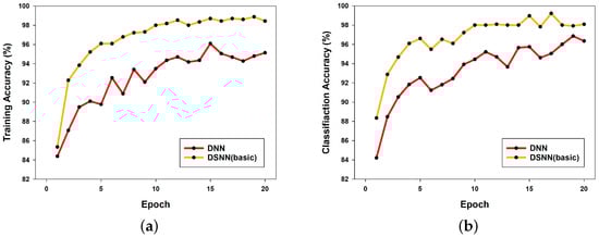
Figure 3.
Comparison of DNN and DSNN performance: (a) training accuracy; (b) classification accuracy.
Similarly, Figure 3b presents the classification results of both models. As observed in the training accuracy comparison, the DSNN achieves higher classification performance than the DNN across all epochs.
Next, Figure 4a presents a comparison between a fully basic DSNN model, which does not incorporate any of the applied techniques (Adam optimizer, dropout, layer normalization, and learning rate scheduler), and a DSNN model with these techniques applied to verify their effectiveness. As a result, the DSNN model without these techniques achieved a maximum accuracy of 68.96% over 20 epochs. In contrast, the DSNN model with these techniques applied achieved an accuracy of 98.78% over 20 epochs, demonstrating the necessity of these applied techniques.
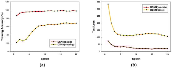
Figure 4.
Comparison of DSNN training accuracy and test loss: (a) training accuracy of DSNN with and without applied techniques; (b) test loss comparison between DSNN (lambda) and DSNN (basic).
Figure 4b shows a comparison of the loss values for both models. The DSNN model with the applied techniques recorded a maximum loss of 73.949 over 20 epochs, whereas the basic DSNN model exhibited a significantly higher maximum loss of 333.3932. This substantial difference in loss values between the two models highlights the impact of the applied techniques.
These results collectively demonstrate the necessity of incorporating the most suitable techniques for optimizing DSNN performance.
Figure 5a presents a comparison of training accuracy between the DSNN models using the proposed modified learning rate scheduler and the conventional lambda learning rate scheduler to verify the effectiveness of the newly introduced approach. The two models differ only in the learning rate scheduler, while all other network configurations remain identical. The graph shows that the DSNN model with the modified learning rate scheduler achieves a higher accuracy than the DSNN model using the lambda learning rate scheduler, particularly during the initial epochs (i.e., the first 10 epochs). The average accuracy over the first 10 epochs is 95.9215% for the DSNN with the modified learning rate scheduler and 94.8093% for the DSNN with the lambda learning rate scheduler, demonstrating the effectiveness of the proposed approach.
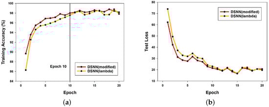
Figure 5.
Comparison of DSNN performance with modified and lambda learning rate schedulers: (a) training accuracy; (b) test loss.
Similarly, Figure 5b compares the test loss of both models. The results show that the DSNN model with the modified learning rate scheduler consistently achieves lower loss across almost all epochs, further validating the effectiveness of the proposed learning rate scheduling method.
Figure 6a presents a graph measuring the training accuracy of the DSNN with the modified learning rate scheduler applied, evaluated across different numbers of hidden layers. In this graph, the model with the highest number of hidden layers (four hidden layers) exhibits the highest accuracy in most cases over the 20 epochs. Additionally, after extending the simulation to 30 epochs, the four-hidden-layer model achieved the highest training accuracy of 99.913% and the highest test accuracy of 98.787%.
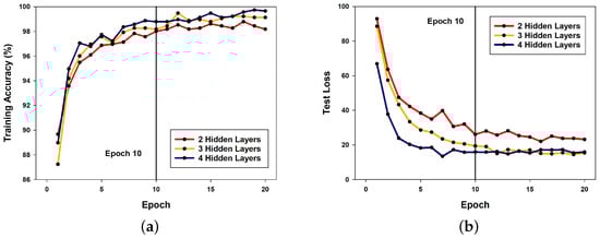
Figure 6.
Comparison of DSNN performance with different numbers of hidden layers: (a) training accuracy; (b) training loss.
Similarly, Figure 6b compares the test loss of the three models. Once again, the model with four hidden layers demonstrates the lowest loss across most epochs, reinforcing the observation that deeper neural networks tend to yield higher performance.
To further evaluate the effectiveness of the proposed DSNN, a comparative analysis was conducted against two representative models—LeNet-5 and MobileNet v2—on the MNIST dataset. These models were selected due to their similar number of trainable parameters to the DSNN. For a fair comparison, the DSNN was configured with three hidden layers. As shown in Figure 7, both the DSNN and LeNet-5 achieve significantly higher test accuracy than MobileNet v2. In particular, the DSNN achieves a comparable performance to LeNet-5, with a difference of less than 1% in test accuracy.
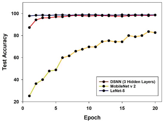
Figure 7.
Comparison of test accuracy on the MNIST dataset using DSNN (3 hidden layers), MobileNet v2, and LeNet-5 over 20 training epochs.
In addition to the MNIST dataset, training and test accuracy were also evaluated on the Fashion-MNIST dataset using DSNN models with two, three, and four hidden layers. As the number of hidden layers increased, the classification accuracy showed consistent improvement. In particular, the model with four hidden layers achieved a maximum test accuracy of 92.19% at epoch 10. The training and test accuracy trends for different model depths are illustrated in Figure 8a and Figure 8b, respectively.
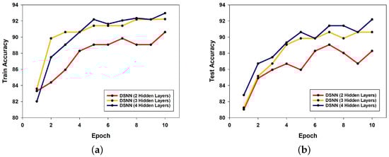
Figure 8.
Comparison of DSNN performance on the Fashion-MNIST dataset with different numbers of hidden layers: (a) training accuracy; (b) test accuracy.
From the perspective of computational efficiency, the proposed two-hidden-layer DSNN exhibits average spike rates of less than 30% in the first hidden layer, second hidden layer, and output layer, thereby yielding an overall average of around 0.24 across epochs. Unlike a conventional dense DNN, where all neurons are involved in computation at every time step, the DSNN performs MAC operations only for the fan-out of neurons that actually fire, leading to a linear reduction in the number of operations proportional to the spike rate. Although the input-to-hidden layer remains densely connected, the use of sparse, event-driven computation in the subsequent layers—with spike activity limited to less than 30% of the neurons at each time step—significantly reduces the computational burden. This sparsity alone led to a reduction in total MAC operations, despite the presence of multiple time steps, clearly demonstrating that temporal expansion is effectively offset by the sparsity of spike events.
4. Discussion
There are several reasons why the DSNN outperforms DNNs. First, the DSNN utilizes temporal information, allowing input patterns to be learned over multiple time steps. Since the membrane potential accumulates over time, information is propagated more effectively. Consequently, unlike DNNs, which rely solely on the output at a single time step, the DSNN generates multiple spikes over time, enabling more stable feature extraction and ultimately achieving higher classification performance.
Moreover, in the case of DNNs, when deep hidden layers or a large number of parameters are used, the activation values of numerous neurons are not reset. This can lead to gradient vanishing or exploding during the backpropagation process. Conversely, in the DSNN, each neuron fires only when its membrane potential exceeds a threshold, and the potential resets upon spiking. This prevents activation values from increasing indefinitely.
Finally, by applying the modified learning rate scheduler to the DSNN, the learning rate is actively adjusted based on the loss gradient during the early epochs. As a result, the DSNN reaches the optimal point more quickly during the initial training phase and can achieve more effective learning in fewer epochs.
Due to these reasons, a DSNN with the modified learning rate scheduler outperforms not only conventional DNNs but also traditional DSNN models.
5. Conclusions
In this paper, we applied a supervised learning approach, using deep learning techniques, to spiking neural networks (SNNs) instead of the conventional unsupervised methods. Additionally, we enhanced the stability of the network and achieved higher performance by incorporating optimization techniques best suited for SNNs, such as the Adam optimizer, dropout, and layer normalization. Furthermore, we proposed an improved DSNN by introducing a modified learning rate scheduler that enables faster training and more rapid convergence to the optimal point compared to conventional DSNNs.
The proposed DSNN with the modified learning rate scheduler was validated on the MNIST dataset. The results demonstrated that it achieved higher accuracy than both conventional DSNNs and deep neural networks (DNNs) that employed the same optimization techniques. In particular, the application of the modified learning rate scheduler significantly improved performance during the early training phase.
In future research, we plan to further enhance DSNN performance by introducing a new surrogate gradient descent and conducting FPGA-based implementation and simulation for more precise validation.
Author Contributions
S.-H.C. and D.-S.K. contributed equally to this work. All authors have read and agreed to the published version of the manuscript.
Funding
This work was supported by the IITP (Institute of Information & Communications Technology Planning & Evaluation)–ITRC (Information Technology Research Center) grant funded by the Korea government (specifically, the Ministry of Science and ICT) (IITP-2025-RS-2024-00438007).
Institutional Review Board Statement
Not applicable.
Informed Consent Statement
Not applicable.
Data Availability Statement
The data are contained within the article.
Conflicts of Interest
The authors declare no conflicts of interest.
References
- Strubell, E.; Ganesh, A.; McCallum, A. Energy and policy considerations for modern deep learning research. In Proceedings of the AAAI Conference on Artificial Intelligence, New York, NY, USA, 7–8 February 2020; Volume 34, pp. 13693–13696. [Google Scholar]
- Thompson, N.C.; Greenewald, K.; Lee, K.; Manso, G.F. The computational limits of deep learning. arXiv 2020, arXiv:2007.05558. [Google Scholar]
- Anthony, L.F.W.; Kanding, B.; Selvan, R. Carbontracker: Tracking and predicting the carbon footprint of training deep learning models. arXiv 2020, arXiv:2007.03051. [Google Scholar]
- Nguyen, A.; Yosinski, J.; Clune, J. Deep neural networks are easily fooled: High confidence predictions for unrecognizable images. In Proceedings of the IEEE Conference on Computer Vision and Pattern Recognition, Boston, MA, USA, 7–12 June 2015; pp. 427–436. [Google Scholar]
- Serre, T. Deep learning: The good, the bad, and the ugly. Annu. Rev. Vis. Sci. 2019, 5, 399–426. [Google Scholar] [CrossRef] [PubMed]
- Glorot, X.; Bengio, Y. Understanding the difficulty of training deep feedforward neural networks. In Proceedings of the Thirteenth International Conference on Artificial Intelligence and Statistics, JMLR Workshop and Conference Proceedings, Sardinia, Italy, 13–15 May 2010; pp. 249–256. [Google Scholar]
- Bair, W.; Koch, C. Temporal precision of spike trains in extrastriate cortex of the behaving macaque monkey. Neural Comput. 1996, 8, 1185–1202. [Google Scholar] [CrossRef] [PubMed]
- Eshraghian, J.K.; Ward, M.; Neftci, E.O.; Wang, X.; Lenz, G.; Dwivedi, G.; Bennamoun, M.; Jeong, D.S.; Lu, W.D. Training spiking neural networks using lessons from deep learning. Proc. IEEE 2023, 111, 1016–1054. [Google Scholar] [CrossRef]
- Burkitt, A.N. A review of the integrate-and-fire neuron model: I. Homogeneous synaptic input. Biol. Cybern. 2006, 95, 1–19. [Google Scholar] [CrossRef]
- Hodgkin, A.L.; Huxley, A.F. A quantitative description of membrane current and its application to conduction and excitation in nerve. J. Physiol. 1952, 117, 500. [Google Scholar] [CrossRef] [PubMed]
- Izhikevich, E.M. Simple model of spiking neurons. IEEE Trans. Neural Netw. 2003, 14, 1569–1572. [Google Scholar] [CrossRef] [PubMed]
- Diehl, P.U.; Cook, M. Unsupervised learning of digit recognition using spike-timing-dependent plasticity. Front. Comput. Neurosci. 2015, 9, 99. [Google Scholar] [CrossRef] [PubMed]
- Wu, Y.; Deng, L.; Li, G.; Zhu, J.; Shi, L. Spatio-temporal backpropagation for training high-performance spiking neural networks. Front. Neurosci. 2018, 12, 331. [Google Scholar] [CrossRef] [PubMed]
- Kasabov, N.K. NeuCube: A spiking neural network architecture for mapping, learning and understanding of spatio-temporal brain data. Neural Netw. 2014, 52, 62–76. [Google Scholar] [CrossRef] [PubMed]
- Neftci, E.O.; Mostafa, H.; Zenke, F. Surrogate gradient learning in spiking neural networks: Bringing the power of gradient-based optimization to spiking neural networks. IEEE Signal Process. Mag. 2019, 36, 51–63. [Google Scholar] [CrossRef]
- Fang, W.; Yu, Z.; Chen, Y.; Masquelier, T.; Huang, T.; Tian, Y. Incorporating learnable membrane time constant to enhance learning of spiking neural networks. In Proceedings of the IEEE/CVF International Conference on Computer Vision, Montreal, BC, Canada, 11–17 October 2021; pp. 2661–2671. [Google Scholar]
- Hinton, G.; Srivastava, N.; Swersky, K. Neural networks for machine learning lecture 6a overview of mini-batch gradient descent. Sci. Res. 2012, 14, 2. [Google Scholar]
- Kingma, D.P.; Ba, J. Adam: A method for stochastic optimization. arXiv 2014, arXiv:1412.6980. [Google Scholar]
- Hinton, G.E.; Srivastava, N.; Krizhevsky, A.; Sutskever, I.; Salakhutdinov, R.R. Improving neural networks by preventing co-adaptation of feature detectors. arXiv 2012, arXiv:1207.0580. [Google Scholar]
- Shannon, C.E. A mathematical theory of communication. Bell Syst. Tech. J. 1948, 27, 379–423. [Google Scholar] [CrossRef]
- Bridle, J. Training stochastic model recognition algorithms as networks can lead to maximum mutual information estimation of parameters. In Proceedings of the 3rd International Conference on Neural Information Processing Systems, Cambridge, MA, USA, 1 January 1989; Volume 2. [Google Scholar]
- Li, Z.; Arora, S. An exponential learning rate schedule for deep learning. arXiv 2019, arXiv:1910.07454. [Google Scholar]
- Loshchilov, I.; Hutter, F. Sgdr: Stochastic gradient descent with warm restarts. arXiv 2016, arXiv:1608.03983. [Google Scholar]
Disclaimer/Publisher’s Note: The statements, opinions and data contained in all publications are solely those of the individual author(s) and contributor(s) and not of MDPI and/or the editor(s). MDPI and/or the editor(s) disclaim responsibility for any injury to people or property resulting from any ideas, methods, instructions or products referred to in the content. |
© 2025 by the authors. Licensee MDPI, Basel, Switzerland. This article is an open access article distributed under the terms and conditions of the Creative Commons Attribution (CC BY) license (https://creativecommons.org/licenses/by/4.0/).