A Multi-Scale Fusion Convolutional Network for Time-Series Silicon Prediction in Blast Furnaces

Abstract

In steel production, the blast furnace is a critical element. In this process, precisely controlling the temperature of the molten iron is indispensable for attaining efficient operations and high-grade products. This temperature is often indirectly reflected by the silicon content in the hot metal. However, due to the dynamic nature and inherent delays of the ironmaking process, real-time prediction of silicon content remains a significant challenge, and traditional methods often suffer from insufficient prediction accuracy. This study presents a novel Multi-Scale Fusion Convolutional Neural Network (MSF-CNN) to accurately predict the silicon content during the blast furnace smelting process, addressing the limitations of existing data-driven approaches. The proposed MSF-CNN model extracts temporal features at two distinct scales. The first scale utilizes a Convolutional Block Attention Module, which captures local temporal dependencies by focusing on the most relevant features across adjacent time steps. The second scale employs a Multi-Head Self-Attention mechanism to model long-term temporal dependencies, overcoming the inherent delay issues in the blast furnace process. By combining these two scales, the model effectively captures both short-term and long-term temporal dependencies, thereby enhancing prediction accuracy and real-time applicability. Validation using real blast furnace data demonstrates that MSF-CNN outperforms recurrent neural network models such as Long Short-Term Memory (LSTM) and the Gated Recurrent Unit (GRU). Compared with LSTM and the GRU, MSF-CNN reduces the Root Mean Square Error (RMSE) by approximately 22% and 21%, respectively, and improves the Hit Rate (HR) by over 3.5% and 4%, highlighting its superiority in capturing complex temporal dependencies. These results indicate that the MSF-CNN adapts better to the blast furnace’s dynamic variations and inherent delays, achieving significant improvements in prediction precision and robustness compared to state-of-the-art recurrent models.

1. Introduction

Most global steel production relies on the blast furnace (BF) process, where this core apparatus drives iron extraction from ore [1]. The BF’s core role is transforming iron oxides in ore into liquid hot metal through sustained smelting. As depicted in Figure 1, its structure comprises five critical zones: throat, shaft, belly, bosh, and hearth [2].

During operation, iron ore, coke, and flux are fed into the furnace top, while preheated, oxygen-enriched air is injected from the bottom. Rising gases react with coke via complex physicochemical reactions, generating reducing agents that convert ore-based iron oxides into molten iron. These gases, after temperature and compositional adjustments, form BF gas as a byproduct. Concurrently, descending raw materials undergo heating, reduction, and melting, ultimately yielding liquid iron and slag through sequential transformations [3].

Precise thermal regulation of molten iron is vital for efficient smelting, directly impacting iron quality, production efficiency, and process stability [4,5]. Optimal temperature ensures complete reaction of raw materials and maintains iron fluidity, which are critical for consistent smelting outcomes. However, direct measurement of (BF) internal thermal states is challenged by sensor limitations [6].

Consequently, silicon content in hot metal serves as a key proxy for furnace temperature, reflecting BF thermal dynamics [7]. Elevated silicon levels often signal excessive coke usage, leading to increased fuel consumption and uneven reactions that degrade iron quality. Conversely, low silicon indicates depleted energy reserves, raising the risk of cold furnace conditions and potential equipment damage [8].

Given these complexities, developing accurate silicon content prediction models has become a pivotal technical hurdle in ironmaking, bridging the gap between indirect thermal monitoring and real-time process control.

The silicon content in hot metal can be precisely measured via sample collection and offline analysis. Nevertheless, this approach is plagued by substantial latency, failing to provide actionable insights for real-time control of BF operations during smelting [2]. Alternatively, first-principle models based on the fundamental principles of the BF ironmaking process can deliver real-time silicon content, but they are computationally expensive and the predictions lack sufficient accuracy [9]. The fast advancements in sensor technologies and detection methods enable the collection of vast amounts of process data, which facilitates the implementation of predictive models [10,11,12]. The data-driven methods for predicting silicon content have been widely studied [13,14,15,16,17], with artificial neural networks and their variants being common modeling approaches. For instance, Saxen and Pettersson, as well as Nurkkala et al., developed feedforward neural network models to predict hourly hot metal silicon content, utilizing 15 and 16 BF variables, respectively [7,18]. Cardoso et al. employed a Bayesian regularized artificial neural network to predict the silicon content of hot metal, achieving the best prediction results by adjusting the number of neurons in the hidden layer [19]. In addition, Zhou et al. proposed the sliding-window Takagi–Sugeno fuzzy neural network model, which enhances prediction accuracy by updating the training data at specified intervals, demonstrating significant improvements in hit rate and mean square error when compared to the traditional T-S FNN model [20]. Furthermore, Jiale Song et al. developed a silicon content prediction model for hot metal in BF smelting by optimizing a back-propagation neural network with the flower pollination algorithm and principal component analysis, leading to enhanced prediction accuracy and overall performance compared to non-optimized models [21].

Moreover, recent advancements in multi-objective evolutionary algorithms (MOEAs) have driven the development of diverse multi-objective ensemble learning methodologies, particularly in the construction of high-performance predictive models [2,22,23,24]. For example, Zhang et al. proposed the CL-MOEEL algorithm for silicon content prediction, improving prediction performance by enabling information exchange between the base learner training and ensemble stages [25].

Building upon the identified challenges in the current data-driven prediction models for silicon content, the following research gaps are specifically addressed:

• Inadequate handling of long time delays in BF processes: Despite the success of data-driven methods in silicon content prediction, the inherent long time delays in BF operations—arising from its complex dynamic system and physical reactions with significant lags [26]—have not been sufficiently addressed in many existing models.
• Neglect of historical time-step dependencies: Most data-driven approaches rely on instantaneous input variables for predictions, failing to capture the time delay effects where current silicon content is influenced by inputs from previous time steps. This limits their ability to reflect evolving system states over time [27].
• Suboptimal prediction accuracy under dynamic conditions: Traditional short-term models exhibit reduced effectiveness in rapidly changing process conditions, as they cannot adequately account for time-lagged influences, thereby hindering real-time adjustments for BF operations.

To better handle the above issues, we propose a Multi-Scale Fusion Convolutional Neural Network (MSF-CNN) model for predicting silicon content in the BF ironmaking process. This model aims to handle the limitations of existing methods in time delays and long-term dependencies, by integrating information from different scales to enhance prediction accuracy and real-time performance.

Specifically, our model extracts features from two different scales: Scale 1 converts the features of each time step into two-dimensional vectors and applies the Convolutional Block Attention Module (CBAM) to capture local information between adjacent time steps by automatically weighting the importance of the features, thereby extracting more critical temporal features. Scale 2 treats the features of each time step in the time series as independent representations and uses a Multi-Head Self-Attention to capture the complex dependencies between time steps, particularly modeling long-term dependencies. By extracting features at these two scales and fusing them, we can comprehensively utilize information at different levels to fully capture the temporal variations in the BF ironmaking process. Finally, the effectiveness and superiority of the proposed method in silicon content prediction are validated through tests on actual BF data. The main contributions can be summarized as follows:

• The Multi-scale Fusion Convolutional Neural Network Model is proposed: An innovative model combining multi-scale feature extraction and deep learning is proposed to tackle the problem of silicon content prediction in the BF ironmaking process. This model effectively captures the complex dynamic characteristics in both long-term and short-term dependencies in the time-series data by fusing information from two different scales;
• The CBAM and Multi-Head Self-Attention Mechanism are introduced: During the feature extraction process, the CBAM and Multi-Head Self-Attention Mechanism are leveraged to enhance the model’s feature selection ability when processing BF smelting data. The CBAM helps automatically weight the importance of features, while the MSA further strengthens the model’s capability to capture the complex relationships between time steps in the time series.

The structure of this article is as follows: Section 2 provides a brief overview of the CBAM and MSA. Section 3 presents a detailed explanation of the proposed algorithm. Section 4 discusses the experiments and results based on both benchmark and real-world industrial data. Finally, Section 5 concludes the article.

2. Preliminaries

This section provides essential background and technical foundations for the subsequent research. It first outlines the challenges posed by BF data characteristics—such as time delays and variable coupling—and the limitations of traditional modeling methods. Subsequently, key techniques leveraged in this study, including the CBAM and self-attention mechanism, are introduced to address these challenges, laying the groundwork for the proposed approach.

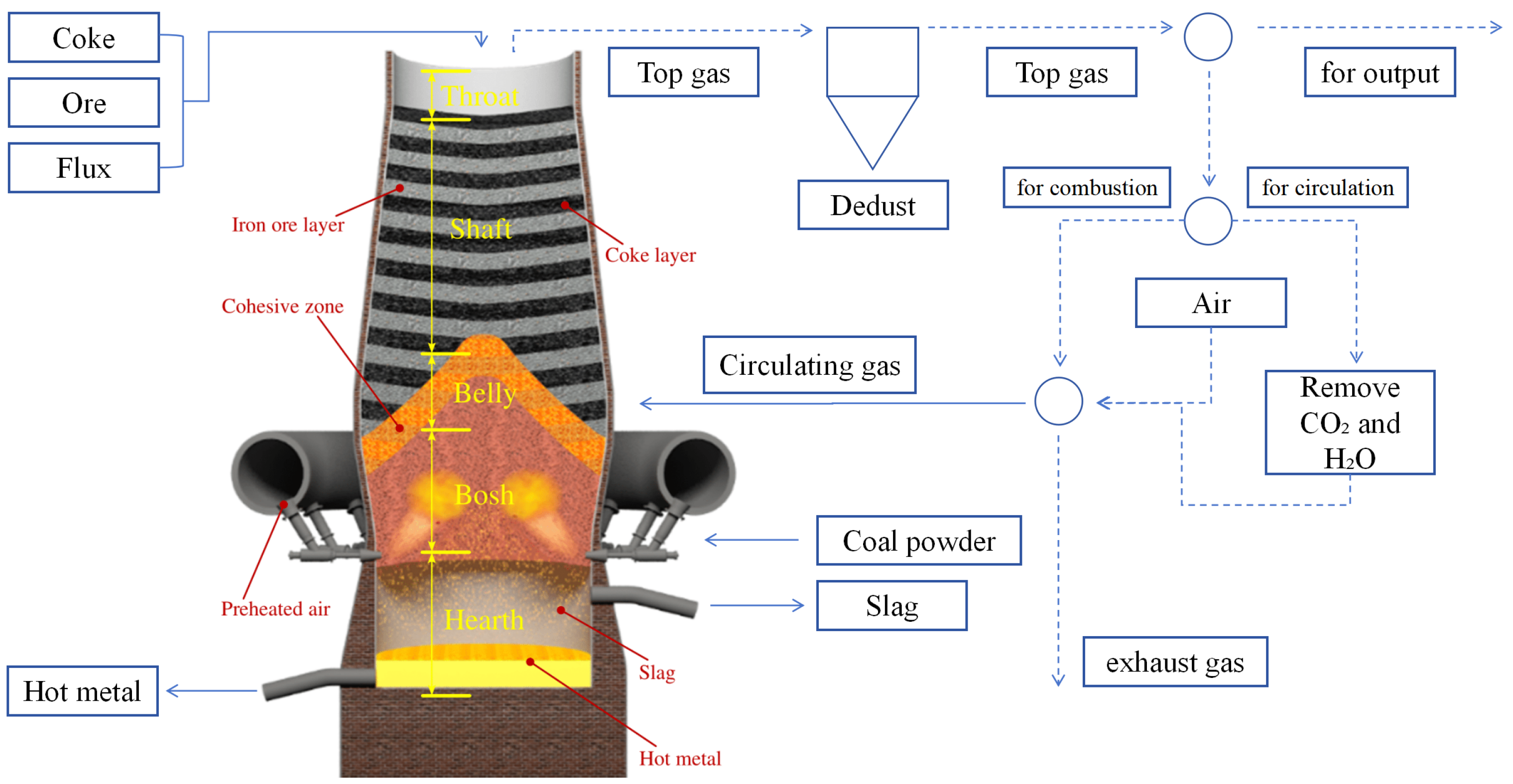
2.1. Challenges of Blast Furnace Data and Traditional Methods

Industrial process data, such as those from BF, typically exhibit significant time-delay characteristics, where the current state often depends on input data from a previous time period. Additionally, such data are strongly coupled, with multiple variables being interdependent, making it difficult to treat them in isolation. This presents several challenges for models designed to process such data, particularly in capturing long-term temporal dependencies and complex inter-variable relationships.

Traditional CNNs mainly extract local features from time series data through convolution operations. However, for time-delay data, CNNs have a limited receptive field that cannot cover information over long time spans, restricting their ability to capture temporal dependencies. Furthermore, CNNs often overlook the sequential dependencies between time steps, which undermines their performance in modeling time series data. To address these issues, recurrent neural networks (RNNs) and their variants [28], such as LSTM networks and GRUs [29,30], are widely applied to time series forecasting tasks. While they can handle temporal data and capture long-term dependencies, their inherent structural characteristics make them vulnerable to gradient vanishing, especially for long sequences. Moreover, LSTMs and GRUs struggle to fully capture the complex relationships between variables, limiting their effectiveness in complex systems such as BFs.

For the above reasons, many methods based on multi-scale feature fusion have been proposed to improve prediction accuracy, proving to be very effective [31,32,33]. For example, Wang et al. proposed a multi-objective convolutional neural network ensemble learning method with multiscale data fusion (MOCNNEL-MSDF) to improve product quality prediction in iron and steel enterprises, addressing the limitations of existing methods by incorporating both macroscopic and mesoscopic data [34].

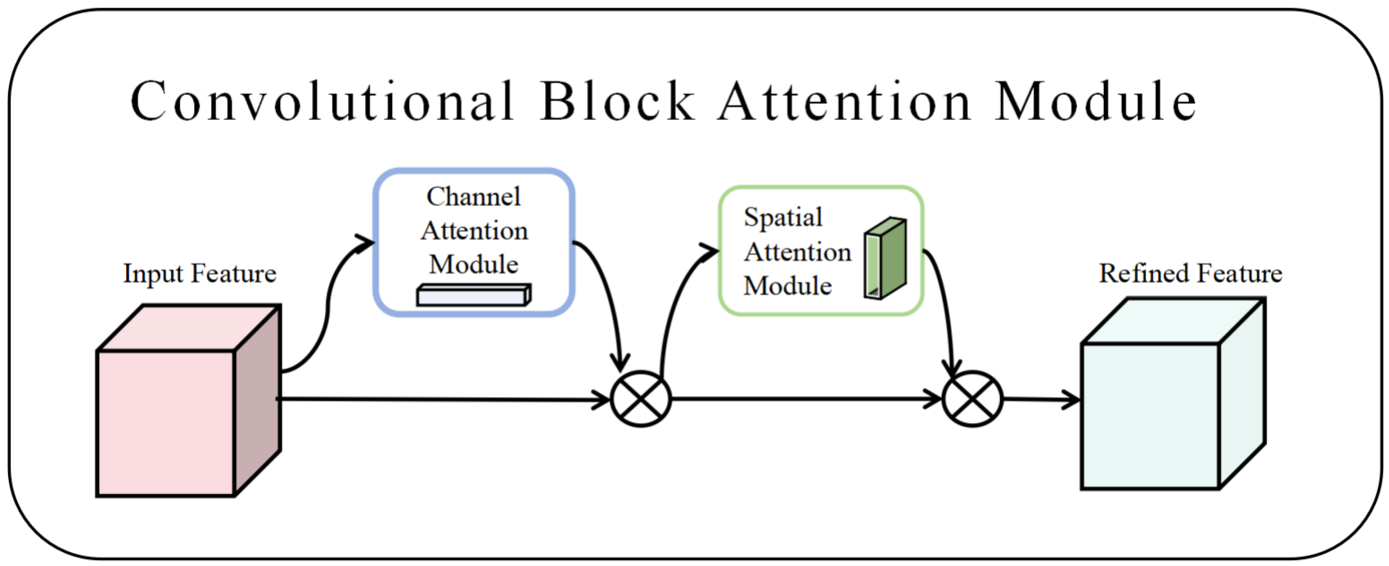
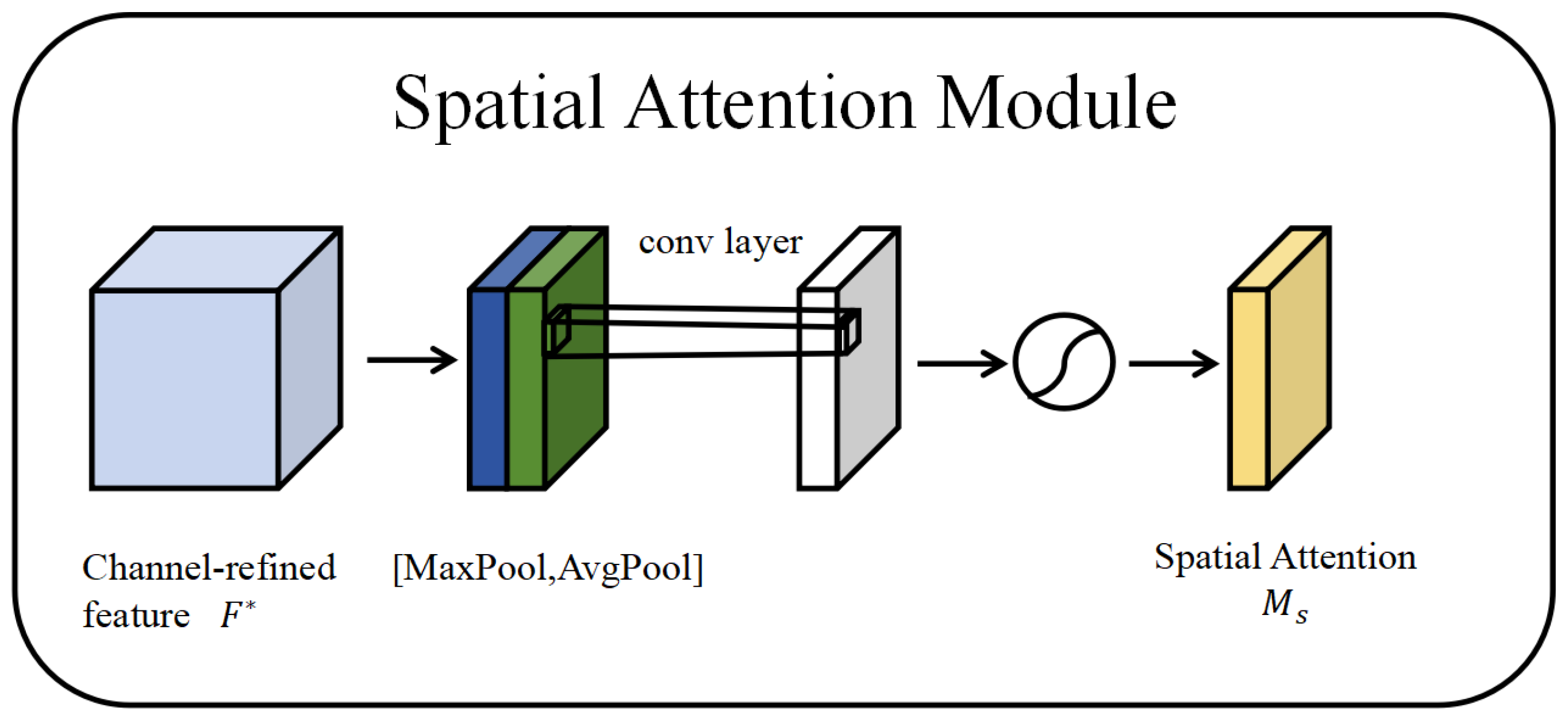
2.2. Convolutional Block Attention Module

The CBAM integrates spatial and channel dimensions to prioritize critical features while suppressing irrelevant information. Following feature map generation by a convolutional neural network, the CBAM derives weight maps from both channel and spatial perspectives, which are then element-wise multiplied with the input feature map to enable adaptive learning. As a lightweight and versatile component, it seamlessly integrates into various convolutional neural networks for end-to-end training [35], with its architecture visualized in Figure 2.

Taking the feature map F as input, the channel attention module (CAM) produces a 1D vector $M_c$, quantifying the importance of each channel through adaptive weighting. Concurrently, the spatial attention module (SAM) generates a 3D map $M_s$, highlighting region-specific relevance by encoding spatial dependencies. The sequential operations are outlined as follows.

$$F^{\prime }=M_c\left(F\right)\otimes F$$

(1)

$$F^{″}=M_s\left(F^{\prime }\right)\otimes F^{\prime }$$

(2)

The CAM emphasizes the relevant content within the input data. The CBAM utilizes two types of pooling operations: max-pooling and average-pooling. These pooling methods help in extracting high-level features, and by using different pooling strategies, a more diverse set of high-level features can be captured. Figure 3 illustrates the structure of the CAM.

The channel attention vector is given by:

$$M_c\left(F\right)=\sigma (MLP\left(AvgPool\left(F\right)\right)+MLP\left(MaxPool\left(F\right)\right))$$

(3)

The SAM, on the other hand, focuses on identifying the critical spatial locations, supplementing the CAM. Figure 4 shows the SAM.

The spatial attention map is calculated as:

$$Ms\left(F\right)=\sigma \left(Conv\right(\left[AvgPool\right(F); MaxPool(F\left)\right]\left)\right)$$

(4)

Here, $\sigma (·)$ represents the sigmoid function, $MaxPool(·)$ refers to max-pooling, $AvgPool(·)$ refers to average-pooling, $MLP(·)$ stands for a multi-layer perceptron, and $Conv(·)$ indicates a 3D convolutional layer.

2.3. Self-Attention Mechanism

The MSA is a key component of the Transformer architecture, which enables the model to process input data by mapping it into multiple subspaces [36]. In these subspaces, the model computes feature representations and corresponding attention scores for each part of the input data. This mechanism focuses the model on the most relevant information in relation to the query vectors, improving its ability to handle sequential data. The structure of the MSA is illustrated in Figure 5.

Let the input to the MSA be denoted as $\mathit{X}$ $\in {\mathbb{R}}^{T\times d}$, where T is the sequence length and d is the input dimension. The input is first linearly transformed into queries Q $\in {\mathbb{R}}^{T\times d_a}$, keys $K\in {\mathbb{R}}^{T\times d_a}$, and values $V\in {\mathbb{R}}^{T\times d_a}$ using learned weight matrices:

$$\mathit{Q}=\mathit{X}·W_q$$

(5)

$$\mathit{K}=\mathit{X}·W_k$$

(6)

$$\mathit{V}=\mathit{X}·W_v$$

(7)

Here, $d_a$ represents the dimensionality of the queries, keys, and values. The MSA mechanism divides the queries, keys, and values into h distinct heads, with each head processing a different part of the input.

For each head, the cosine similarity $A_i$ is computed between the query $Q_i$ and the key $K_i$. This similarity is then normalized using the Softmax function:

$$A_i=Softmax\left({\displaystyle \frac{Q_i·K_i^T}{\sqrt{d_a/h}}}\right), i=1,2,\dots ,h$$

(8)

The output for each head is obtained by multiplying the attention scores $A_i$ with the corresponding values $V_i$:

$$O_i=A_i·V_i, i=1,2,\dots ,h$$

(9)

Finally, the outputs from all h attention heads are concatenated and passed through a non-linear activation function to produce the final output:

$$O=f\left(\mathrm{Concat}\left(O_1,O_2,\dots ,O_h\right)\right)$$

(10)

where $f(·)$ denotes the non-linear activation function that is applied to the concatenated outputs.

3. Methodology

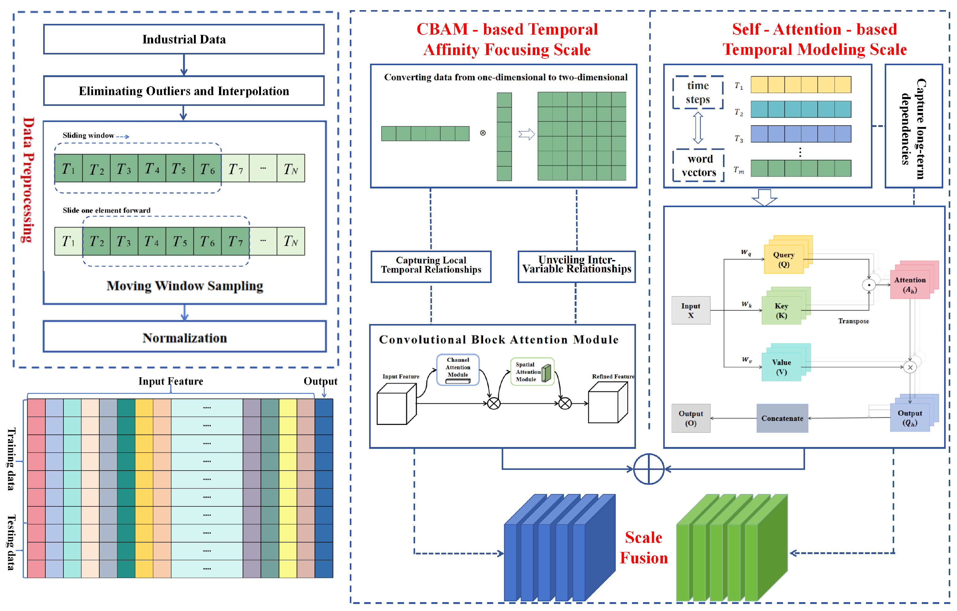
3.1. Overall Framework of MSF-CNN

In this section, we outline the architectural design of MSF-CNN, engineered to model temporal dependencies at both local and global scales within time-series data. The model has two key scales: the CBAM-based Temporal Affinity Focusing Scale for local temporal feature extraction and the self-attention-based Temporal Modeling Scale for capturing global temporal dependencies. These two scales are then fused to enhance the predictive performance of the model. The main structure of the model is illustrated in Figure 6, which demonstrates the process and computation of two temporal modeling scales.

• CBAM-based Temporal Affinity Focusing Scale: By introducing the CBAM, this scale focuses on critical features within local temporal windows, capturing local temporal dependencies. The CBAM module employs both the channel and SAM to selectively focus on the most important features, thereby enhancing the modeling capability of local time series data.
• Self-Attention-based Temporal Modeling Scale: Building on this, the self-attention mechanism is used to model global temporal dependencies. Unlike traditional RNN/LSTM/GRU methods, self-attention allows the model to freely capture dependencies across long time spans on a global scale. By calculating the relationships between time steps, the self-attention mechanism effectively mitigates the gradient vanishing problem and can comprehensively capture complex interactions between variables.

These two temporal modeling scales work in tandem, modeling time series data at both the local and global levels, which significantly improves its ability to process complex temporal data.

3.2. CBAM-Based Temporal Affinity Focusing Scale

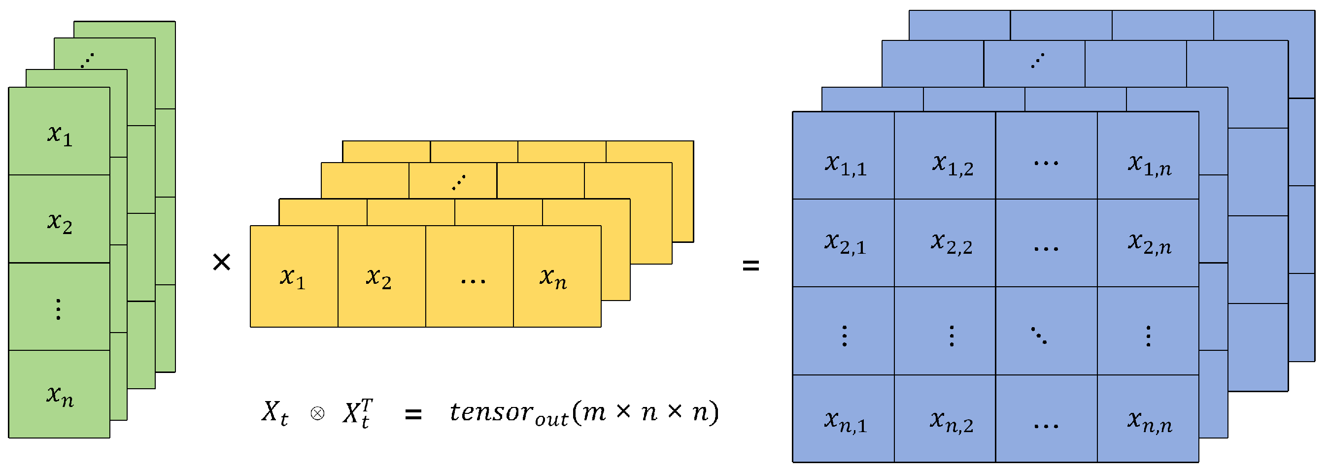
3.2.1. Temporal Feature Enhancement via Outer Product Operation

In this model, we enhance the attention to important features in time series data by introducing the CBAM. First, to more effectively model the coupling relationships between variables at each time step, we use the outer product operation to transform the one-dimensional feature vector of each time step into a two-dimensional feature matrix. This helps capture the interactions between different variables at each time step.

Assuming the feature of each time step is an ${\mathbb{R}}^n$ vector, we use the outer product operation to map it into a ${\mathbb{R}}^{n\times n}$ matrix, where each element represents the interaction between two variables at that time step.

$${\mathit{X}}_{\mathit{t}}=x_t\otimes x_t^T$$

(11)

By applying the outer product operation, the model can explicitly capture the nonlinear relationships between different variables within each time step, providing richer feature information for the subsequent attention mechanism. Figure 7 illustrates this operation visually.

3.2.2. Attention Mechanism Optimization in Time Series Processing

Optimizing the attention mechanism in time series data processing, especially in complex systems like BF, can effectively capture the dynamic relationships between time steps and different variables. The goal of this optimization is to enhance the model’s sensitivity to important information by adjusting the weights of features, thereby improving prediction accuracy. After performing the outer product operation, we can generate tensors and pass them through the CBAM, which integrates both CAM and SAM to collaboratively enhance the model’s predictive ability.

The CAM aims to assign weights to different channels to reflect the importance of each time step for the current prediction task. Each time step is treated as a feature channel, and the CAM learns the weights for these feature channels to strengthen the model’s focus on the important channels.

Let $\mathit{X}\in {\mathbb{R}}^{m\times n\times n}$ represent the input feature map, where m is the number of time steps, n is the feature dimension.

The CAM focuses on adjusting the weights of each channel to enhance the model’s attention to important channels.

The global average pooling and global max pooling are firstly applied to the input feature $map\mathit{X}$:

$$F_{avg}=AvgPool\left(\mathit{X}\right),F_{max}=MaxPool\left(\mathit{X}\right)$$

(12)

where $F_{avg}$ and $F_{max}$ have dimensions $m\times 1\times 1$, representing global information for each channel.

Next, we pass $F_{avg}$ and $F_{max}$ through shared fully connected layers (typically two FC layers) and apply a nonlinear activation function such as ReLU to process the information, ultimately obtaining the channel attention weights:

$$M_{channel}=\sigma \left(FC\left(ReLU\left(FC\left(F_{avg}+F_{max}\right)\right)\right)\right)$$

(13)

where $M_{channel}\in {\mathbb{R}}^{m\times 1\times 1}$ represents the attention weights for each channel, and $\sigma$ is the sigmoid activation function, outputting weights between 0 and 1.

Finally, the input feature map $\mathit{X}$ is adjusted by multiplying it with the channel attention weights $M_{channel}$:

$${\mathit{X}}_{\mathit{out}}=\mathit{X}·M_{channel}$$

(14)

This way, important time steps receive higher weights, better capturing the time-lag characteristics of the BF system.

The CAM dynamically adjusts the input feature map based on the importance of each time step, highlighting the time steps relevant to the current prediction task. For systems like BF, which exhibit significant time-lag effects, different time steps have varying impacts on the current prediction task. The CAM helps capture these impacts accurately.

The SAM assigns weights to the different features at each time step, identifying which features are crucial for the current prediction task. It applies attention across the spatial dimensions, highlighting features that significantly contribute to the prediction task.

As in the CAM, we first apply global average pooling and global max pooling to ${\mathit{X}}_{out}$, extracting spatial information:

$$F_{avg\_spatial}=AvgPool\left({\mathit{X}}_{out}\right),F_{max\_spatial}=MaxPool\left({\mathit{X}}_{out}\right)$$

(15)

The resulting $F_{avg\_spatial}$ and $F_{max\_spatial}$ have dimensions $1\times H\times W$, representing spatial information for each time step.

We combine the two pooled outcomes and feed them into a convolutional layer so as to generate the SAM map $M_{spatial}$:

$$M_{spatial}=\sigma \left(Conv\left(F_{avg\_spatial}\oplus F_{max\_spatial}\right)\right)$$

(16)

where the concatenation operation ⊕ produces a tensor that is passed through a convolutional layer to learn the spatial attention weights. The output $M_{spatial}$ has dimensions $1\times n\times n$, representing spatial attention for each time step.

Finally, the spatial attention weights $M_{spatial}$ are applied to $X_{out}$:

$$X_{final}=X_{out}·M_{spatial}$$

(17)

This allows the model to identify which features at each time step are most important, further enhancing focus on key features.

The SAM deeply explores which features at each time step contribute the most to the final prediction, especially in systems like BF, where complex interactions occur between variables. This mechanism helps the model capture which features have a significant impact on the prediction of silicon content at a given moment.

The integrated approach of using both channel and SAM enhances the prediction accuracy for complex industrial systems like BF. The CAM captures local temporal relationships by identifying the impact of each time step on the current prediction, as different time steps contribute differently to the final outcome. Meanwhile, the SAM uncovers inter-variable relationships by weighting the interactions between features, highlighting those that significantly affect the prediction. By combining these mechanisms, the model can flexibly adjust feature weights, focusing on critical time steps and features, ultimately improving both the robustness and accuracy of the prediction. This approach enables a more effective capture of dynamic features, leading to better overall performance in predicting complex systems.

3.3. Self-Attention-Based Temporal Modeling Scale

In the prediction task of silicon content in the BF, time-series data are often deeply influenced by historical states and exhibits strong time lag effects. Traditional models, such as LSTM and other recurrent neural networks, can capture time dependencies but still face challenges in modeling long-term dependencies. To address this issue, this study introduces the MSF, which improves prediction accuracy by capturing global temporal dependencies. The self-attention mechanism has excellent modeling capabilities, allowing it to directly model correlations between different time points over long time steps without relying on recursive transmission mechanisms. The introduction of this mechanism enables a more effective capture of nonlinear relationships and global information in the silicon content time-series data.

Assume that our dataset consists of operational features of the BF at multiple time steps. The data at each time step represent real-time monitoring information during the BF operation, including raw material composition, gas flow, furnace temperature, and so on.

The core idea of the self-attention mechanism is to calculate the correlations between each element in a sequence and use these correlations as weighting factors to adjust the representation of each element. Specifically, given an input sequence $\mathit{X}=$$\left[x_1,x_2,\dots ,x_m\right]\in {\mathbb{R}}^{m\times n}$, where m is the time step and n is the feature dimension, the traditional attention mechanism first calculates the similarity between the query $\mathit{Q}$ and the key $\mathit{K}$ to obtain a weighted matrix (attention matrix), and then uses this weighted matrix to adjust the value $\mathit{V}$.

To input these time-step features into the self-attention mechanism, we first need to perform linear transformations to generate the query, key, and value matrices. By multiplying with learned weight matrices, we convert the input matrix into $\mathit{Q}$, $\mathit{K}$ and $\mathit{V}$ matrices:

$$\mathit{Q}=\mathit{X}·W_Q,\mathit{K}=\mathit{X}·W_K,\mathit{V}=\mathit{X}·W_V$$

(18)

Here, $W_Q,W_K$, and $W_V$ are learned weight matrices, each used to generate the queries, keys, and values, respectively. The dimensions of these matrices are $d_k$, which helps capture the relationships between different time steps in the BF operation. Through this transformation, we map the original BF operational features $\mathit{X}$ into a new representation space, allowing us to capture relationships between different time steps.

The essence of the self-attention mechanism is calculating the similarity between the query and the key, which helps capture correlations between different time steps. For example, the raw material ratio at certain time steps might have a greater impact on the silicon content prediction at later time steps, while temperature changes at other time steps may be less relevant. Therefore, by calculating the dot product between the query and key, we apply the softmax function to obtain the attention weights between each time step:

$$\alpha =softmax\left({\displaystyle \frac{\mathit{Q}{\mathit{K}}^T}{\sqrt{d_k}}}\right)$$

(19)

These attention weights $\alpha$ help us identify the importance of features at different time steps in the BF operation for the current silicon content prediction.

Once the attention weights are calculated, we apply them to the value matrix V and compute a weighted sum to obtain the final output, which incorporates the weighted features from all time steps:

$$Output=\alpha \mathit{V}$$

(20)

This weighted sum process essentially combines the global dependencies of the features at each time step, helping the model better understand and predict the temporal changes in silicon content in the BF.

In the prediction task of silicon content in the BF, considering that there may be multiple layers of dependencies between different time steps, we use the MSA. Through parallel computation in multiple heads, different dimensions of temporal relationships can be captured in different subspaces. Each head independently computes its corresponding query, key, and value, and the outputs of all heads are concatenated and linearly transformed to achieve the final output:

$$MultiHead(\mathit{Q},\mathit{K},\mathit{V})=Concat\left(hea{d}_1,hea{d}_2,\dots ,hea{d}_h\right)W_O$$

(21)

This approach allows us to consider the BF operational data from multiple perspectives, thereby capturing more potential temporal dependencies.

In the BF silicon content prediction task, during the training process, Since the prediction of silicon content is a regression problem, we use a loss function such as Mean Squared Error to measure the prediction error of the model, and optimize the weight matrices through backpropagation. The loss function is defined as:

$$L={\displaystyle \frac{1}{N}}\sum _{i=1}^N{\left({\widehat{y}}_i-y_i\right)}^2$$

(22)

where ${\widehat{y}}_i$ is the predicted silicon content obtained through the self-attention mechanism, and $y_i$ is the actual silicon content. By minimizing this loss, the model automatically adjusts the weight matrices for the queries, keys, and values, thereby capturing the relationships between each time step and the global context and generating the final attention matrix $M\in R^{m\times n\times n}$.

By utilizing the self-attention mechanism, we can effectively capture the relationships between BF operational features at different time steps, thus improving the accuracy of silicon content prediction. The MSA further enhances the model’s ability to learn multi-dimensional temporal dependencies across different time steps. During the training process, the model continuously updates the weights via backpropagation, allowing the features at each time step to better reflect in the final silicon content prediction.

3.4. Fusion of Local and Global Temporal Scales

In the MSF-CNN model, local temporal features and global temporal dependencies are fused through concatenation to enhance the model’s predictive capability. Specifically, the CBAM-based Temporal Affinity Focusing Scale extracts key features within local temporal windows and leverages the outer product operation to capture interactions between variables. The CBAM module is employed to optimize the importance of these features. This scale primarily focuses on the dynamic changes between adjacent time steps in the time series, ensuring the accurate capture of short-term details and local dependencies. At the same time, the Self-Attention-based Temporal Modeling Scale effectively models global temporal dependencies using the self-attention mechanism. This overcomes the limitations of traditional methods in capturing long-range dependencies, enabling the model to capture global dynamic changes across time steps.

The fusion of these two scales is not merely a simple concatenation but adopts an adaptive weight fusion method suitable for different industrial scenarios, comprehensively integrating local and global information to enhance the model’s temporal modeling capability. After fusion, the model can simultaneously leverage local details and global trends, thus exhibiting stronger adaptability and higher prediction accuracy when handling complex time series data. The local scale provides fine-grained variations within short-term time series data, while the global scale enhances the model’s understanding of long-term dependencies. This fusion approach enables the MSF-CNN to achieve significant performance improvements across a variety of complex applications.

Through this feature fusion, MSF-CNN can provide more accurate and stable time series predictions in domains such as industrial process control and environmental monitoring. The concatenation of the two scales enables the model to handle both instantaneous changes and long-term patterns, thereby offering a more comprehensive capability for time series analysis.

4. Experimental Results and Discussion

In this part, we verified the efficacy of the suggested MSF-CNN approach for predicting the silicon content. The data utilized were sourced from a leading iron and steel production enterprise in China. We employed real-world data gathered during the ironmaking procedure. The MSF-CNN model was then contrasted with other forecasting models. Subsequently, we delved deeply into its performance and effectiveness. Moreover, ablation tests were carried out to assess the contribution of every part of the model. This step guarantees a thorough comprehension of the model’s advantages and drawbacks.

4.1. Experimental Settings

Owing to the intricacy of the ironmaking process, numerous process variables influence the fluctuations in the silicon content of the molten iron. Drawing on the ironmaking mechanism, expert insights, and the references presented in Section 1, 46 process variables were chosen for the prediction. These variables are detailed in

Table 1. Partial input features for silicon content prediction model.

Input Feature	Unit
Furnace Waist Average Temperature	°C
Furnace Waist Temperature Range	°C
Top Furnace Pressure	kPa
Top Furnace Temperature	°C
Top Furnace Gas CO Content	%
Top Furnace Gas H2 Content	%
Sintered Ore	%
Wind flow	${\mathrm{m}}^3/\min$
Coal Injection Rate	t/h
Actual Air Velocity	$\mathrm{m}/\mathrm{s}$
Oxygen-Enriched Pressure	kPa
Oxygen Enrichment Rate	${\mathrm{m}}^3/\min$
${\mathrm{Al}}_2{\mathrm{O}}_3$	%
$\mathrm{CaO}$	%
$\mathrm{MgO}$	%
${\mathrm{SiO}}_2$	%
C	%

. To prepare the data, we performed preprocessing operations as outlined in Equation (23), which included normalization and imputation of missing values. For each sampling time of silicon content, we collected time-series data of the selected process variables over a 6-h period using a moving-window sampling method with a 60 min interval. The sliding window had a length of 6, resulting in an input feature dimension of 276 for each sample. Each sample was structured as a tensor with the shape (6, 46), which served as the initial input for the model. The dataset was split into training and testing sets, with 80% of the samples used for training and 20% reserved for testing. To minimize the impact of randomness and ensure the stability of the results, all experiments were repeated 10 times, and the final performance metrics were obtained by averaging the results across these runs.The silicon-content time series, arranged by taping number, is shown in Figure 8.

$$V_{norn}={\displaystyle \frac{V-V_{min}}{V_{max}-V_{min}}}$$

(23)

In the experiments, the development environment consisted of Python 3.8.19, with PyTorch version 2.3.1 and CUDA 11.8 for GPU acceleration. The platform was equipped with an AMD Ryzen 7 5800H CPU (3.20 GHz) and an NVIDIA GeForce RTX 3060 GPU, providing the necessary computational power for the tasks.

Additionally, five performance metrics were used, namely Root Mean Square Error (RMSE), Mean Absolute Error (MAE), Hit Rate (HR), Coefficient of Determination ($R^2$), and Correlation Coefficient (${\rho }_{\mathrm{corr}}$), which are defined as follows:

• $RMSE$:

  $$\mathbf{RMSE}=\sqrt{{\displaystyle \frac{1}{N}}\sum _{i=1}^N{\left(y^{t_i}-{\widehat{y}}^{t_i}\right)}^2}$$

  (24)
• $MAE$:

  $$\mathbf{MAE}={\displaystyle \frac{1}{N}}\sum _{i=1}^N\left|y^{t_i}-{\widehat{y}}^{t_i}\right|$$

  (25)
• $PredictionHR$:

  $$\begin{array}{cc}\hfill & \mathbf{HR}={\displaystyle \frac{1}{N}}\sum _{i=1}^N{I}_{e_i}\hfill \end{array}$$

  (26)
• $CoefficientofDetermination\left(R^2\right)$:

  $$R^2=1-{\displaystyle \frac{{\sum }_{i=1}^N{\left(y^{t_i}-{\widehat{y}}^{t_i}\right)}^2}{{\sum }_{i=1}^N{\left(y^{t_i}-{\overline{y}}^{t_i}\right)}^2}}$$

  (27)
• $CorrelationCoefficient\left({\rho }_{corr}\right)$:

  $${\rho }_{\mathrm{corr}}={\displaystyle \frac{1}{N}}{\displaystyle \frac{{\sum }_{i=1}^N(y^{t_i}-{\overline{y}}^{t_i})\left(\left({\widehat{y}}^{t_i}-{\overline{\widehat{y}}}^{t_i}\right)\right)}{\mathrm{var}\left(y^{t_i}\right)\mathrm{var}\left({\widehat{y}}^{t_i}\right)}}$$

  (28)

4.2. Model Performance Optimization

To determine the optimal hyperparameters for the best model performance, we first set the basic hyperparameters based on preliminary experimental results, including: learning rate (0.001, using Adam optimizer), batch size (32), number of training epochs (50), regularization (dropout rate of 0.3), and L2 regularization coefficient (0.0005). These hyperparameters remained constant throughout the experiments to secure stable outcomes.

In the MSA, the number of attention heads is a crucial hyperparameter that influences the model’s performance. The number of heads controls the number of parallel attention mechanisms, affecting both the model’s ability to express input information and the computational cost. Therefore, tuning the number of heads is key to improving model performance. We trained the model with different numbers of heads and evaluated its performance on the validation and test sets to determine the optimal configuration. Specifically, we compared five different head configurations: 2 heads, 4 heads, 8 heads, 16 heads, and 32 heads. For each configuration, other hyperparameters were kept constant to eliminate potential interference, ensuring the comparability of the results. In each experiment, the model was trained for 50 epochs, and loss values were computed on both the training and validation sets, with performance ultimately evaluated on the test set. The results show that as the number of attention heads increased, the training error, validation error, and test error all gradually decreased, as illustrated in Figure 9. Among all configurations, the model with 32 heads achieved the best performance, with MSE = 0.0625, MAE = 0.25, and HR = 90.1%.

4.3. Experimental Results

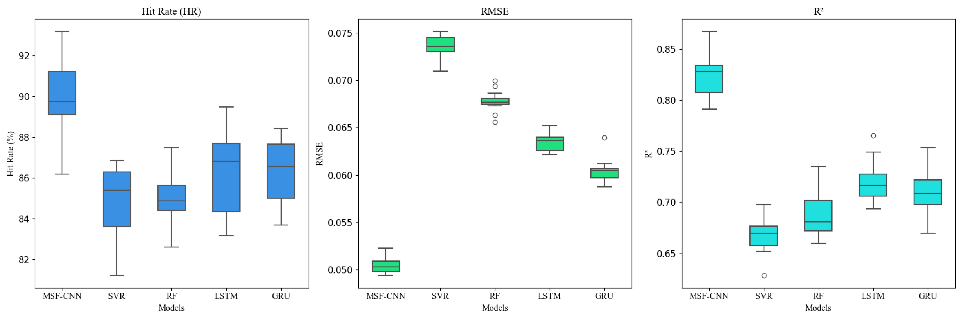
4.3.1. Comparison with Baseline Models

To evaluate the effectiveness and advantages of the proposed model, we compare it against several baseline models commonly used for time-series prediction. These include Support Vector Regression (SVR), LSTM, GRU, and Random Forest Regression (RF) [37]. Each of these models has distinct characteristics and strengths in handling time-series data, and this comparison offers a comprehensive evaluation of the MSF-CNN model’s performance.

The input data for all models are the same raw time-series data used in the MSF-CNN model to ensure fairness in the comparison. Additionally, the parameter selection and training settings for all comparison models are aligned with those of our proposed model to ensure the comparability of results. Specifically, the SVR model uses an RBF kernel with a penalty parameter C = 1.0 and an error tolerance $ϵ=0.01$, with other parameters set to their default values. The LSTM model consists of two LSTM layers, each with 64 hidden units, and uses the Adam optimizer with a learning rate of 0.001, a batch size of 32, and 100 training epochs. A dropout rate of 0.2 is applied as a regularization technique to prevent overfitting. The GRU model follows a similar structure to the LSTM, with two layers of 64 hidden units, and uses the same optimizer, learning rate, and dropout settings. The Random Forest Regression model is configured with 100 trees, a maximum depth of 10, and a minimum sample split of 2.The comparison of the true values and predicted values for different models is shown in Figure 10.

As shown in

Table 2. Performance metrics comparison for different models.

Model	MSF-CNN	SVR	RF	LSTM	GRU
RMSE	5.08 $\times {10}^{-2}$	7.36 $\times {10}^{-2}$	6.75 $\times {10}^{-2}$	6.33 $\times {10}^{-2}$	6.01 $\times {10}^{-2}$
MAE	0.0522	0.0699	0.0683	0.0622	0.0599
HR	90.02%	84.74%	85.53%	86.37%	86.71%
R2	8.30 $\times {10}^{-1}$	6.68 $\times {10}^{-1}$	6.91 $\times {10}^{-1}$	7.11 $\times {10}^{-1}$	7.07 $\times {10}^{-1}$
${\rho }_{corr}$	0.8203	0.7075	0.7132	0.7543	0.7522

and Figure 11, the MSF-CNN model outperforms all other models in the prediction of [SI], achieving optimal results in RMSE, HR, and other performance metrics, demonstrating its superiority in handling complex process data. Specifically, the MSF-CNN achieved the lowest RMSE of 5.08 $\times {10}^{-2}$, which is 2.28 $\times {10}^{-2}$, lower than that of SVR (7.36 $\times {10}^{-2}$), representing an improvement of approximately 31%. Similarly, in terms of MAE, the MSF-CNN showed a value of 0.0522, which is a 25% reduction compared to SVR (0.0699). Additionally, the MSF-CNN achieved an HR (accuracy) of 90.02%, outperforming SVR (84.74%) by 5.28% and RF (85.53%) by 4.49%. In terms of the coefficient of determination, MSF-CNN exhibited a value of 0.8203, which is 16% higher than SVR (0.7075) and 15% higher than RF (0.7132), indicating superior model fitting ability. The GRU and LSTM also showed strong performance, with values of 0.7522 and 0.7543, respectively, although they were still slightly lower than MSF-CNN. Regarding the correlation coefficient, MSF-CNN demonstrated the highest value of 8.30 $\times {10}^{-1}$, which is 24% higher than SVR (6.68 $\times {10}^{-1}$) and 20% higher than RF (6.91 $\times {10}^{-1}$), reflecting stronger correlation between its predictions and the actual values. Overall, the MSF-CNN demonstrated superior performance across all key metrics, showing substantial improvements compared to other models. In particular, the MSF-CNN achieved approximately 30% better performance in RMSE and MAE, and a 5% improvement in HR, highlighting its robust predictive capability and higher accuracy. In contrast, SVR and RF showed relatively weaker performance, especially in terms of prediction error and accuracy. The specific training process is shown in Figure 12.

Next, we present a thorough analysis on the performance and weaknesses of each model. SVR faces performance bottlenecks when handling large-scale, high-dimensional data due to the need for selecting suitable kernel functions and parameters, causing a sharp rise in computational costs as data size increases, making it difficult to model complex data. Additionally, SVR struggles to capture temporal dependencies and dynamic changes, leading to larger prediction errors, especially in multivariate cases. While RF performs well at capturing nonlinear features, it is a tree-based model that cannot effectively model dynamics or long-term dependencies in time series data due to its limited ability to understand temporal correlations and sequential information. On the other hand, LSTM and the GRU, as variants of recurrent neural networks (RNNs), excel at capturing temporal dependencies through internal memory mechanisms, which makes them suitable for time-series prediction. However, they are less efficient than convolutional neural networks (CNNs) at extracting static features and complex nonlinear relationships, and are likely to encounter gradient vanishing and exploding issues when handling long sequences.

The MSF-CNN model demonstrates superior performance in predicting the silicon content in BF, particularly with respect to accuracy and generalization. The key innovation of this model lies in its ability to capture the time-lag relationships inherent in the BF process through a multi-scale approach, effectively leveraging attention mechanisms to extract features from different time scales. By combining these two scales, the MSF-CNN model can effectively capture both static and dynamic features from the data, providing a richer representation of the time dependencies. This is particularly important for BF systems, which inherently exhibit time-lagged behaviors.

The results clearly demonstrate that the MSF-CNN outperforms other models in terms of predictive accuracy and robustness. Unlike traditional models such as SVR and RF, which struggle to capture temporal dynamics and nonlinear relationships, the MSF-CNN model leverages its multi-scale structure and attention mechanisms to extract both local and global features, leading to superior performance.

4.3.2. Ablation Study

To assess the effectiveness of the MSF-CNN model, a series of ablation experiments were conducted to evaluate the contribution of each component to the overall prediction accuracy. Specifically, we compared four distinct model configurations by progressively removing or replacing key modules within the model. The first configuration, MSF-CNN, represents the full model, which integrates two scales: Scale 1 (CBAM) and Scale 2 (MSA). Scale 1 captures local temporal dependencies through the CBAM, while Scale 2 leverages the MSA mechanism to model global temporal dependencies. This dual-scale approach enables the model to capture both short-term and long-term temporal features, thus enhancing predictive performance. To isolate the effect of each individual component, three additional variants were tested. The second model, NoCBAM-CNN, removes the CBAM module in Scale 1 and retains only the MSA module in Scale 2, allowing for an evaluation of the role of CBAM in modeling local temporal dependencies. The third model, NoMSA-CNN, eliminates the MSA module in Scale 2 and preserves only the CBAM module in Scale 1, thus testing the contribution of the MSA mechanism in capturing global temporal dependencies. Finally, the Baseline-CNN model serves as a simple control, which removes both Scale 1 and Scale 2 feature extraction mechanisms, relying solely on a traditional CNN for feature extraction and prediction. This baseline model provides a point of comparison to evaluate the impact of multi-scale and attention mechanisms on model performance.The specific experimental results are shown in

Table 3. Results of the ablation study.

Metric	MSF-CNN	NoCBAM-CNN	NoMSA-CNN	Baseline-CNN
RMSE	5.22 $\times {10}^{-2}$	6.36 $\times {10}^{-2}$	6.72 $\times {10}^{-2}$	7.73 $\times {10}^{-2}$
MAE	0.0568	0.0677	0.0696	0.0793
HR	90.1%	85.68%	82.15%	74.37%
R2	8.33 $\times {10}^{-1}$	6.35 $\times {10}^{-1}$	6.42 $\times {10}^{-1}$	6.02 $\times {10}^{-1}$
${\rho }_{\mathrm{corr}}$	0.8347	0.7183	0.7241	0.7005

.

4.4. Discussion

The MSF-CNN proposed in this study effectively addresses the prediction challenges posed by the dynamic time-varying and delayed characteristics in the BF smelting process through a dual-scale temporal feature fusion strategy, demonstrating significant advantages in the real-time prediction accuracy of silicon content. Experimental results show that the model achieves hierarchical modeling of complex temporal dependencies through the combination of CBAM local attention and self-attention mechanisms, achieving over 20% improvement in key performance indicators compared to traditional recurrent neural networks and providing a more reliable intelligent prediction tool for industrial process monitoring.

However, there are still directions to be explored for the model’s practical engineering applications. Although this study verifies the effectiveness of the multi-scale fusion architecture, future research can further focus on optimizing the model’s computational efficiency—such as enhancing real-time inference capabilities through lightweight design or hardware adaptation—to better meet the low-latency and high-reliability deployment requirements of industrial control systems. Additionally, while the built-in attention mechanism provides a potential interpretable path for the prediction process, systematic analysis of feature importance and visual representation of decision logic still need to be deepened. Constructing an interpretability framework combined with domain knowledge, such as quantifying the impact of key time steps or visualizing multi-scale feature interactions, will help enhance operators’ trust in model predictions and promote its practical application in high-value industrial scenarios. These research directions not only strengthen the theoretical completeness of the model but also accelerate its transformation from experimental validation to engineering implementation, providing more comprehensive technical support for the digital upgrading of intelligent steel production.

5. Conclusions

In this study, we presented a novel Multi-Scale Fusion Convolutional Neural Network (MSF-CNN) for predicting the silicon content in molten iron during the blast furnace process. By addressing the limitations of traditional prediction models, the MSF-CNN combines two distinct temporal scales: a Convolutional Block Attention Module for capturing short-term temporal dependencies and a Multi-Head Self-Attention mechanism for modeling long-term dependencies. This dual-scale approach enables the model to effectively handle the dynamic nature and inherent delays of the blast furnace process, resulting in improved prediction accuracy and stability. The validation of the MSF-CNN model using real-world blast furnace data showed its superior performance compared to conventional prediction techniques. Notably, the MSF-CNN outperformed traditional methods in both accuracy and robustness, making it highly adaptable to the complex, fluctuating conditions of the blast furnace.

The proposed model’s success in predicting silicon content underlines the potential of deep learning-based approaches in industrial process monitoring. Future work could explore further optimization of the MSF-CNN architecture, as well as its application to other critical variables in the blast furnace. Ultimately, the MSF-CNN framework can contribute to the development of smarter, more efficient steel production processes, aligning with the growing trend of digitalization and automation in the steel industry.

References

1. Saxén, H.; Gao, C.; Gao, Z. Data-Driven Time Discrete Models for Dynamic Prediction of the Hot Metal Silicon Content in the Blast Furnace—A Review. IEEE Trans. Ind. Inform. 2013, 9, 2213–2225. [Google Scholar] [CrossRef]
2. Wang, X.; Hu, T.; Tang, L. A Multiobjective Evolutionary Nonlinear Ensemble Learning with Evolutionary Feature Selection for Silicon Prediction in Blast Furnace. IEEE Trans. Neural Netw. Learn. Syst. 2021, 33, 2080–2093. [Google Scholar] [CrossRef] [PubMed]
3. Dong, X.F.; Yu, A.B.; Burgess, J.M.; Pinson, D.; Chew, S.; Zulli, P. Modelling of Multiphase Flow in Ironmaking Blast Furnace. Ind. Eng. Chem. Res. 2009, 48, 214–226. [Google Scholar] [CrossRef]
4. Kuang, S.; Li, Z.; Yu, A. Review on Modeling and Simulation of Blast Furnace. Steel Res. Int. 2018, 89, 1700071. [Google Scholar] [CrossRef]
5. Gupta, S.; French, D.; Sakurovs, R.; Grigore, M.; Sun, H.; Cham, T.; Hilding, T.; Hallin, M.; Lindblom, B.; Sahajwalla, V. Minerals and Iron-Making Reactions in Blast Furnaces. Prog. Energy Combust. Sci. 2008, 34, 155–197. [Google Scholar] [CrossRef]
6. Zhou, P.; Li, W.; Wang, H.; Li, M.; Chai, T. Robust Online Sequential RVFLNs for Data Modeling of Dynamic Time-Varying Systems with Application of an Ironmaking Blast Furnace. IEEE Trans. Cybern. 2020, 50, 4783–4795. [Google Scholar] [CrossRef]
7. Saxén, H.; Pettersson, F. Nonlinear Prediction of the Hot Metal Silicon Content in the Blast Furnace. ISIJ Int. 2007, 47, 1732–1737. [Google Scholar] [CrossRef]
8. Jian, L.; Gao, C. Binary Coding SVMs for the Multiclass Problem of Blast Furnace System. IEEE Trans. Ind. Electron. 2013, 60, 3846–3856. [Google Scholar] [CrossRef]
9. Zhou, P.; Wang, C.; Li, M.; Wang, H.; Wu, Y.; Chai, T. Modeling error PDF optimization based wavelet neural network modeling of dynamic system and its application in blast furnace ironmaking. Neurocomputing 2018, 285, 167–175. [Google Scholar] [CrossRef]
10. Li, J.; Yang, C.; Li, Y.; Xie, S. A Context-Aware Enhanced GRU Network with Feature-Temporal Attention for Prediction of Silicon Content in Hot Metal. IEEE Trans. Ind. Inform. 2022, 18, 6631–6641. [Google Scholar] [CrossRef]
11. Guo, R.; Liu, H.; Xie, G.; Zhang, Y.; Liu, D. A Self-Interpretable Soft Sensor Based on Deep Learning and Multiple Attention Mechanism: From Data Selection to Sensor Modeling. IEEE Trans. Ind. Inform. 2023, 19, 6859–6871. [Google Scholar] [CrossRef]
12. Guo, R.; Chen, Q.; Tong, S.; Liu, H. Knowledge-Aided Generative Adversarial Network: A Transfer Gradient-Less Adversarial Attack for Deep Learning-Based Soft Sensors. In Proceedings of the 14th Asian Control Conference (ASCC), Dalian, China, 5–8 July2024; pp. 1254–1259. [Google Scholar]
13. Waller, M.; Saxén, H. On the Development of Predictive Models with Applications to a Metallurgical Process. Ind. Eng. Chem. Res. 2000, 39, 982–988. [Google Scholar] [CrossRef]
14. Bhattacharya, T. Prediction of Silicon Content in Blast Furnace Hot Metal Using Partial Least Squares (PLS). ISIJ Int. 2005, 45, 1943–1945. [Google Scholar] [CrossRef]
15. Saxén, H.; Östermark, R. State realization with exogenous variables—A test on blast furnace data. Eur. J. Oper. Res. 1996, 89, 34–52. [Google Scholar] [CrossRef]
16. Östermark, R.; Saxén, H. VARMAX-modelling of blast furnace process variables. Eur. J. Oper. Res. 1996, 90, 85–101. [Google Scholar] [CrossRef]
17. Zeng, J.-S.; Gao, C.-H. Improvement of identification of blast furnace ironmaking process by outlier detection and missing value imputation. J. Process Control 2009, 19, 1519–1528. [Google Scholar] [CrossRef]
18. Nurkkala, A.; Pettersson, F.; Saxén, H. Nonlinear Modeling Method Applied to Prediction of Hot Metal Silicon in the Ironmaking Blast Furnace. Ind. Eng. Chem. Res. 2011, 50, 9236–9248. [Google Scholar] [CrossRef]
19. Cardoso, W.; di Felice, R. Prediction of silicon content in the hot metal using Bayesian networks and probabilistic reasoning. Int. J. Adv. Intell. Inform. 2021, 7, 268–281. [Google Scholar] [CrossRef]
20. Zhou, H.; Yang, C.; Liu, W.; Zhuang, T. A Sliding-Window T-S Fuzzy Neural Network Model for Prediction of Silicon Content in Hot Metal. IFAC Pap. 2017, 50, 14988–14991. [Google Scholar] [CrossRef]
21. Song, J.; Xing, X.; Pang, Z.; Lv, M. Prediction of Silicon Content in the Hot Metal of a Blast Furnace Based on FPA-BP Model. Metals 2023, 13, 918. [Google Scholar] [CrossRef]
22. Zhang, C.; Lim, P.; Qin, A.K.; Tan, K.C. Multiobjective deep belief networks ensemble for remaining useful life estimation in prognostics. IEEE Trans. Neural Netw. Learn. Syst. 2017, 28, 2306–2318. [Google Scholar] [CrossRef] [PubMed]
23. Bui, L.T.; Vu, V.T.; Dinh, T.T.H. A novel evolutionary multi-objective ensemble learning approach for forecasting currency exchange rates. Data Knowl. Eng. 2018, 114, 40–66. [Google Scholar] [CrossRef]
24. Zhang, H.; Zhou, A.; Zhang, H. An evolutionary forest for regression. IEEE Trans. Evol. Comput. 2022, 26, 735–749. [Google Scholar] [CrossRef]
25. Zhang, J.; Zhao, G.; Wang, X. Silicon Content Prediction in Blast Furnace Ironmaking Process Based on Closed-loop Multiobjective Evolutionary Ensemble Learning. IEEE Trans. Instrum. Meas. 2025, 74, 2516715. [Google Scholar] [CrossRef]
26. Liu, C.; Tan, J.; Li, J.; Li, Y.; Wang, H. Temporal Hypergraph Attention Network for Silicon Content Prediction in Blast Furnace. IEEE Trans. Instrum. Meas. 2022, 71, 2521413. [Google Scholar] [CrossRef]
27. Yan, D.; Yang, C.; Sun, S.; Lou, S.; Kong, L.; Zhang, Y. One-Sided Relational Autoencoder with Seasonal-Trend Decomposition to Extract Process Correlations for Molten Iron Quality Prediction. IEEE Trans. Instrum. Meas. 2024, 73, 1002413. [Google Scholar] [CrossRef]
28. Elman, J.L. Finding Structure in Time. Cogn. Sci. 1990, 14, 179–211. [Google Scholar] [CrossRef]
29. Hochreiter, S.; Schmidhuber, J. Long short-term memory. Neural Comput. 1997, 9, 1735–1780. [Google Scholar] [CrossRef]
30. Chung, J.; Gulcehre, C.; Cho, K.; Bengio, Y. Empirical Evaluation of Gated Recurrent Neural Networks on Sequence Modeling. arXiv 2014, arXiv:1412.3555. [Google Scholar] [CrossRef]
31. Jeon, M.; Choi, H.S.; Lee, J.; Kang, M. Multi-scale prediction for fire detection using convolutional neural network. Fire Technol. 2021, 57, 2533–2551. [Google Scholar] [CrossRef]
32. Zhang, M.; Zhou, L.; Jie, J.; Liu, X. A multi-scale prediction model based on empirical mode decomposition and chaos theory for industrial melt index prediction. Chemometrics Intell. Lab. Syst. 2019, 186, 23–32. [Google Scholar] [CrossRef]
33. Li, H.; Zhao, W.; Zhang, Y.; Zio, E. Remaining useful life prediction using multi-scale deep convolutional neural network. Appl. Soft. Comput. 2020, 89, 106113. [Google Scholar] [CrossRef]
34. Wang, X.; Wang, Y.; Tang, L.; Zhang, Q. Multiobjective Ensemble Learning with Multiscale Data for Product Quality Prediction in Iron and Steel Industry. IEEE Trans. Evol. Comput. 2024, 28, 1099–1113. [Google Scholar] [CrossRef]
35. Woo, S.; Park, J.; Lee, J.-Y.; Kweon, I.S. CBAM: Convolutional Block Attention Module. In Proceedings of the European Conference on Computer Vision (ECCV), Munich, Germany, 8–14 September 2018; pp. 3–19. [Google Scholar]
36. Vaswani, A.; Shazeer, N.; Parmar, N.; Uszkoreit, J.; Jones, L.; Gomez, A.N.; Kaiser, Ł.; Polosukhin, I. Attention Is All You Need. Adv. Neural Inf. Process. Syst. 2017, 30, 5998–6008. [Google Scholar]
37. Breiman, L. Random forests. Mach. Learn. 2001, 45, 5–32. [Google Scholar] [CrossRef]
Figure 1. Structure of a typical BF ironmaking process.
Mathematics 13 01347 g001
Figure 2. CBAM network structure diagram.
Mathematics 13 01347 g002
Figure 3. Channel attention module.
Mathematics 13 01347 g003
Figure 4. Spatial attention module.
Mathematics 13 01347 g004
Figure 5. Structure of self-attention mechanism.
Mathematics 13 01347 g005
Figure 6. Framework of MSF-CNN.
Mathematics 13 01347 g006
Figure 7. Schematic diagram of the outer product operation.
Mathematics 13 01347 g007
Figure 8. Time series of silicon content.
Mathematics 13 01347 g008
Figure 9. Impact of attention heads on model performance.
Mathematics 13 01347 g009
Figure 10. Comparison of predicted and true values across models.
Mathematics 13 01347 g010
Figure 11. Box plots of different silicon content prediction models.
Mathematics 13 01347 g011
Figure 12. Convergence curves of different models.
Mathematics 13 01347 g012