Wavelet and Deep Learning Framework for Predicting Commodity Prices Under Economic and Financial Uncertainty

Abstract

The analysis of commodity markets—particularly in the energy and metals sectors—is essential for understanding economic dynamics and guiding decision-making. Financial and economic uncertainty indices provide valuable insights that help reduce price uncertainty. This study employs wavelet analyses and wavelet energy-based measures to investigate the relationship between these indices and commodity prices across multiple time scales. The wavelet approach captures complex, time-varying dependencies, offering a more nuanced understanding of how uncertainty indices influence commodity price fluctuations. By integrating this analysis with predictability measures, we assess how uncertainty indices enhance forecasting accuracy. We further incorporate deep learning models capable of capturing sequential patterns in financial time series into our analysis to better evaluate their predictive potential. Our findings highlight the varying impact of financial and economic uncertainty on the predictability of commodity prices, showing that while some indices offer valuable forecasting information, others display strong correlations without significant predictive power. These results underscore the need for tailored predictive models, as different commodities react differently to the same financial conditions. By combining wavelet-based measures with machine learning techniques, this study presents a comprehensive framework for evaluating the role of uncertainty in commodity markets. The insights gained can support investors, policymakers, and market analysts in making more informed decisions.

1. Introduction

Financial factors and uncertainties related to government policies have emerged as significant drivers of commodity prices, operating independently of traditional supply and demand dynamics. These elements play a crucial role in shaping market behavior and should be carefully considered by investors and producers when making investment and production decisions. In this study, we examine the impact of financial and policy uncertainties on the price distributions of energy and metal commodities, employing advanced mathematical tools, such as wavelet analysis and an energy-based predictability measure, to gain deeper insights into these complex dynamics.

In particular, we examine the impact of financial and economic uncertainty on energy and metal commodity prices using wavelet coherence analysis, the wavelet Kullback–Leibler divergence measure (WEDM), and Long Short-Term Memory (LSTM) models.

A key aspect of this study is the integration of time-frequency analyses and deep learning for financial time series forecasting. By combining wavelet-based divergence measures with machine learning techniques, we enhance our understanding of how macroeconomic uncertainty, financial stress, and market volatility influence commodity price dynamics. Our findings underscore the importance of developing tailored predictive models, as each commodity exhibits distinct responses to varying financial conditions.

While most of the studies on this topic adopt different approaches, this paper investigates how the futures prices of palladium, copper, and heating oil are affected by financial and economic uncertainty using a non-parametric method based on wavelet analysis. Examples of wavelet approaches can be found in some fields of engineering [1,2] and applied mathematics [3,4], in statistics [5,6], and also in financial time series analyses [7,8,9]. Wavelets are useful for analyzing the correlation between time series because they allow researchers to study how the relationship between the series changes over time and across different frequency scales. Unlike traditional correlations, which provide a single value, wavelet analysis helps in revealing whether the correlation is strong or weak at specific times or frequencies (transient changes vs. persistent behaviors). This is especially useful for non-stationary data, where the characteristics of the series change over time [10,11].

In this article, we also employ wavelet energy-based measures to assess the extent to which information from one time series can reduce the uncertainty of another. By combining this approach with correlation analysis, we make it possible to apply these insights to the forecasting of commodity price series while explicitly accounting for financial and economic uncertainty indices.

Beyond examining these relationships, we integrate predictability measures and deep learning-based forecasting models to evaluate how effectively uncertainty indices contribute to improving price predictions. Specifically, we utilize Long Short-Term Memory (LSTM) networks, which are well suited to capturing sequential dependencies in financial time series. This approach allows us to quantify the influence of macroeconomic uncertainty, financial stress, and market volatility on commodity market dynamics.

This article is structured as follows: In Section 1, we have presented the context, objectives, and motivation of this study. This is followed by Section 2, where we review the literature related to our analysis. In Section 3, we introduce the commodities and financial and economic uncertainty indices used in our analysis. Then, in Section 4, we describe the wavelet analysis, wavelet energy-based measures, and the framework used for forecasting. The results obtained from our analysis are presented in Section 5 and Section 6 and are followed by a forecasting analysis. Finally, a discussion and the conclusions are provided in Section 7.

2. Literature Review

The existing literature has examined the role of commodity markets in enhancing portfolio diversification and improving risk management strategies [12,13,14]. Economic conditions and the unpredictability of government policies have become key influencers of commodity prices which operate outside the usual forces of supply and demand. These factors are pivotal in determining market trends and require thorough attention from both investors and producers when planning investments and production strategies.

Previous empirical research has delved into the impact of financial factors and macroeconomic conditions on commodity markets. There is a strand of the literature that examines the issue of the impact of economic policy uncertainty on stock and commodity prices [15,16]. Ref. [17] discovered a predictable relationship between commodity prices and economic policy uncertainty, and ref. [18] showed that the dynamic link between uncertainty and commodity prices varies over time and, moreover, that it was very different before and after the 2008–2009 global financial crisis.

Study [19] found that uncertainty affects various aspects of the economy, potentially influencing pricing and returns in stock markets, which in turn can affect commodity markets.

Financial uncertainty and stress play a significant role in shaping commodity prices. Since investors often consider commodities to be a hedge or safe-haven asset that protects their portfolios from risks, fluctuations in financial markets—such as increased volatility or heightened financial stress—can influence commodity prices through portfolio adjustments and rebalancing. Ref. [20] examined how financial stress spreads across countries and its impact on global economic activity. The study, which covered the period from 1970 to 2012 and analyzed financial stress indices from 20 major economies, found that the correlation between these indices tends to rise significantly during major financial crises. Ref. [21] analyzed the impact of variations in the CBOE Volatility Index (VIX) on commodities’ futures prices and on the future positions held by financial traders, both before and after the recent financial crisis. Its findings revealed that market uncertainty influenced not only trader positioning but also commodity price movements. Ref. [22] investigated the relationship between oil price volatility and global economic uncertainty, using the VIX as a measure. It found that spikes in the VIX are associated with increased volatility in oil prices, suggesting that financial market uncertainty significantly impacts commodity markets. Ref. [23] investigated the transmission of volatility between oil prices and financial stress from 1991 to 2014. The study found that both oil prices and the St. Louis Fed Financial Stress Index (STLFSI) were primarily driven by long-term volatility. Additionally, a shift was observed in risk transmission patterns: before the global financial crisis, volatility flowed from oil prices to financial stress, whereas after the crisis, financial stress became the dominant driver, influencing oil prices. Ref. [24] examined the dynamic relationships between speculative activities, commodity returns, and macroeconomic conditions across five sectors, encompassing 29 commodities. Utilizing weekly data from January 2000 to July 2023, the study highlighted that financial stress indicators, such as the STLFSI, significantly predict commodities’ future returns and the impact on commodities like palladium and copper.

Recent studies have increasingly turned to exploring the complex interplay between economic policy uncertainty, financial stress, and commodity markets. For example, the European Central Bank’s recent interest rate cut underscores the significant influence of trade policy uncertainty on economic conditions, which in turn affect commodity prices. Similarly, fluctuations in oil prices have been linked to uncertainties surrounding U.S. tariff policies and anticipated production changes from major producers, highlighting the sensitivity of commodity markets to geopolitical developments. China’s recent decline in commodity imports further reflects concerns about economic growth and trade tensions, illustrating how macroeconomic factors shape commodity market behavior. These observations are consistent with earlier research showing that financial stress and policy uncertainty play a pivotal role in driving commodity price movements, reinforcing the need for investors and producers to closely monitor these variables when making investment and production decisions.

3. Data

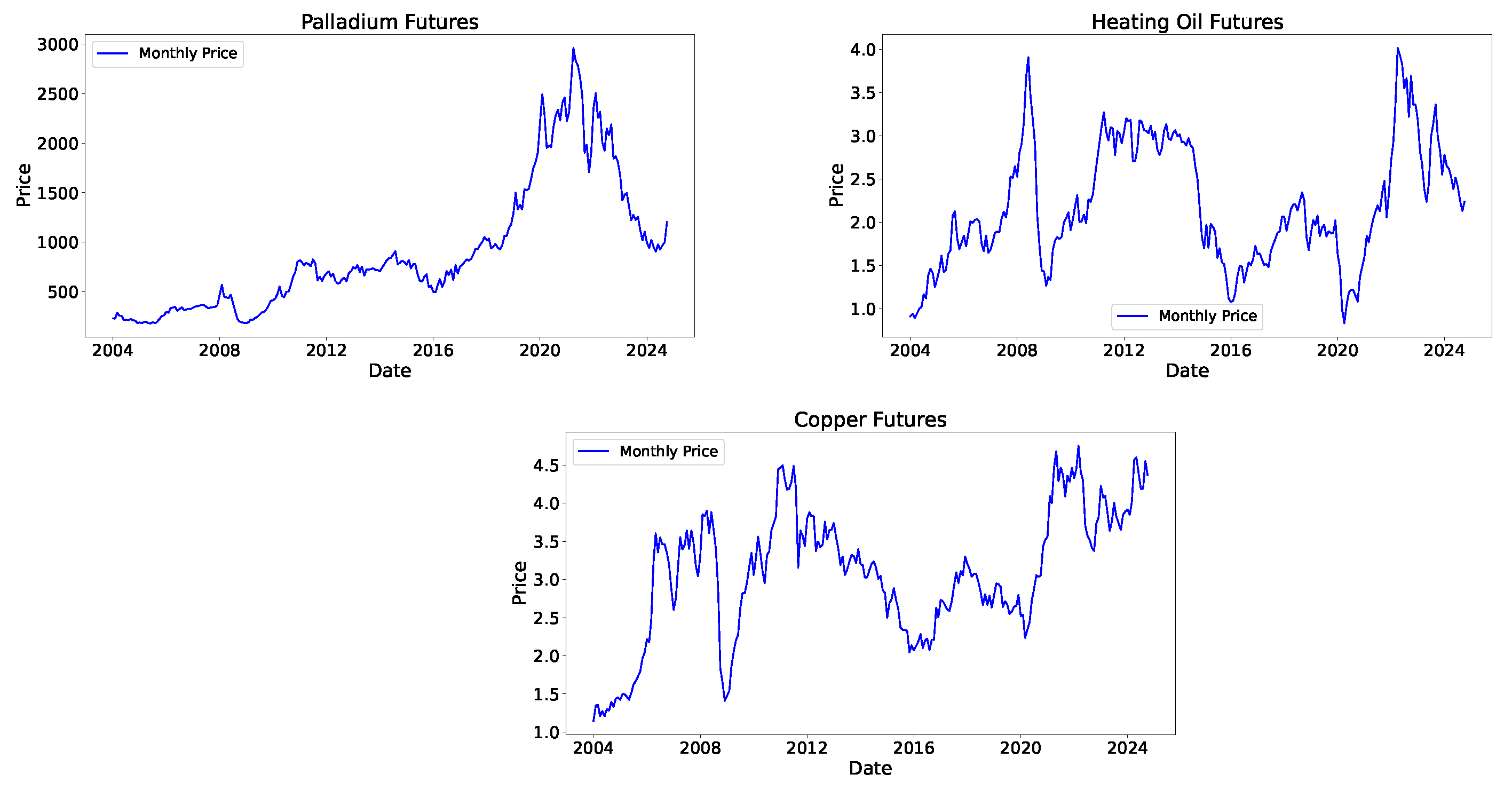
In this article, we analyze monthly data covering the period from January 2004 to September 2024, making a total of 249 observations. Specifically, we focus on the futured prices of three commodities: palladium, heating oil, and copper (all extracted from www.investing.com, accessed on 28 October 2024). The economic and financial significance of palladium, heating oil, and copper, when considered collectively, is both substantial and strategic, with relevance in multiple dimensions. Each of these commodities plays a distinct role in global markets, but their combined value becomes even more pronounced when viewed through the lens of industrial, energy, and technological development.

Palladium serves as a key indicator of the automotive industry and the broader shift toward cleaner energy technologies. Heating oil reflects the health of the energy market, and particularly the balance between seasonal demand and supply dynamics. Copper, often referred to as a barometer of global economic activity, captures trends in industrial performance and infrastructure investments.

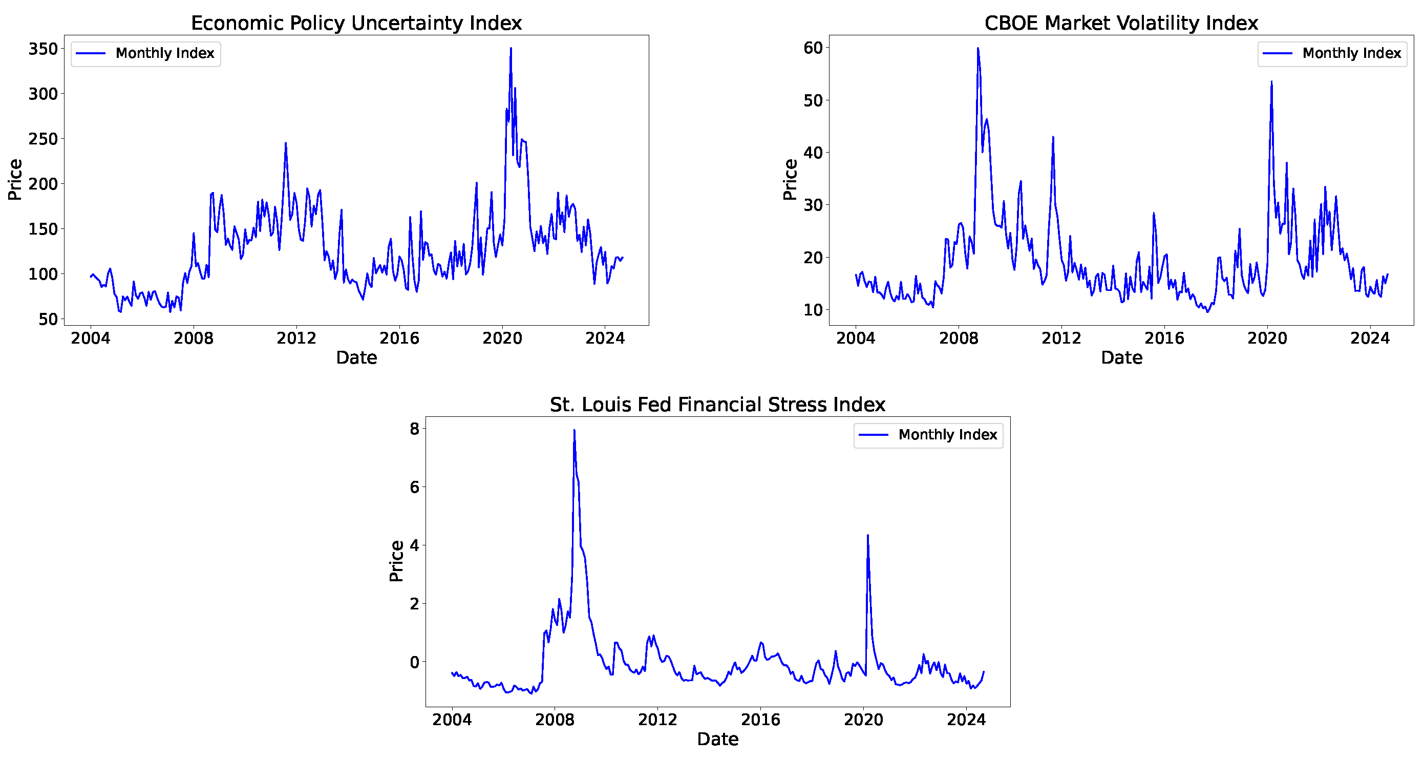
Unlike spot prices, futures prices offer more accurate forecasts by accounting for inflation and effectively reflecting the influence of supply and demand dynamics on commodity prices (for details, see [25,26]). Additionally, we examine three indices: the Economic Policy Uncertainty Index (EPUI) (https://www.policyuncertainty.com/us_monthly.html, accessed on 28 October 2024), the Volatility Index (www.investing.com, accessed on 28 October 2024), and the St. Louis Fed Financial Stress Index (https://fred.stlouisfed.org/series/STLFSI4, accessed on 28 October 2024).

The EPUI is a metric developed to quantify the level of uncertainty regarding economic policies, which can influence the decision-making processes of businesses and households. This index is constructed by analyzing the frequency of specific terms related to the economy, uncertainty, and policy within major newspapers. An increase in the EPU Index indicates heightened uncertainty, which can lead to reduced investment and spending, thereby potentially slowing economic growth. Recent studies have shown that elevated economic policy uncertainty can have a significant negative impact on economic activity, and particularly on investment. For more details, visit https://economy-finance.ec.europa.eu/economic-forecast-and-surveys/economic-forecasts/autumn-2024-economic-forecast-gradual-rebound-adverse-environment/cost-uncertainty-new-estimates_en, accessed on 20 November 2024.

VIX measures the expected volatility of the U.S. stock market over the next 30 days. It is calculated based on options from the S&P 500 Index. It serves as a market sentiment indicator. High VIX values indicate greater uncertainty or fear among investors, while low values suggest more stable markets with lower perceived risk.

The third index we consider is STLFSI, which measures the degree of stress in financial markets and is built to have an average value of zero, which would reflect “normal financial market conditions”. It is a composite index constructed from 18 weekly time series (interest rates, yield spreads, and additional measures such as the CBOE Implied Volatility Index, VIX). High levels in the STLFSI indicate elevated levels of fear or stress.

In Figure 1, the futures prices of three commodities, palladium, heating oil, and copper, can be observed, while in Figure 2, the values of their EPUI, VIX, and STLFSI indices throughout the considered period are shown.

4. Methodology

In this section, we introduce the concept of wavelets and their use in analyzing the time–frequency correlations between two series. Subsequently, we present energy-based measures, closely related to wavelets, that are fundamental for studying the predictability of a series in the time–frequency domain.

4.1. Continuous Wavelet Transform and Power Spectrum

Let us consider a time series $x\left(t\right)\in L^2\left(\mathbb{R}\right)$ and a wavelet function $\phi \left(t\right)\in L^2\left(\mathbb{R}\right)$. The continuous wavelet transform, $W(\tau ,\sigma )$, at the scale $\sigma \in {\mathbb{R}}^{+}$ and with the translation parameter $\tau \in \mathbb{R}$, maps the original time series into a dilated and translated version of the mother wavelet. In particular, it is defined as follows:

$$W(\tau ,\sigma )={\displaystyle \frac{1}{\sqrt{\sigma }}}{\int }_{\mathbb{R}}x\left(t\right)\overline{\phi }\left({\displaystyle \frac{t-\tau }{\sigma }}\right)dt,$$

(1)

where $\phi \left(t\right)$, called the mother wavelet, is a continuous function in both the time and frequency domains and the symbol overline represents the operation of a complex conjugate.

There are several wavelet functions available to play the role of the mother wavelet (see [27]). In particular, in this paper, we make use of the Morlet wavelet, which is defined as follows:

$$\phi \left(t\right)={\displaystyle \frac{1}{\sqrt[4]{\pi }}}{e}^{i{\nu }_{0}t-{\displaystyle \frac{1}{2}}{t}^2}$$

(2)

where ${\nu }_0$ is a dimensionless frequency, t is a dimensionless time, and i represents the imaginary unit.

In our case, the Morlet wavelet is particularly useful because it is a complex function that provides a simple scale-to-frequency conversion ($f\sim 1/s$) when ${\nu }_0=6$ and offers optimal time–frequency localization. Its complex nature enables the extraction of amplitude and phase information, which is crucial for analyzing time delays between the oscillations of two time series [28,29,30].

From Equation (1) we can obtain a measure of the localized variance of the time series, the so-called wavelet power spectrum ($WPS$), which is defined as follows:

$$WP{S}_x={\left|W_x(\tau ,\sigma )\right|}^2.$$

(3)

4.2. Cross-Wavelet Transform and Wavelet Coherence

Now, let us consider two time series $x\left(t\right)$ and $y\left(t\right)$ with continuous wavelet transforms $W_x(\tau ,\sigma )$ and $W_y(\tau ,\sigma )$. The cross-wavelet transform of $x\left(t\right)$ and $y\left(t\right)$ is defined as follows:

$$W_{x,y}(\tau ,\sigma )=W_x(\tau ,\sigma )\overline{W_y(\tau ,\sigma )}.$$

(4)

Starting with this equation, we can define the cross-wavelet power spectrum ($CWS$) as follows:

$$CW{S}_{x,y}=\left|W_{x,y}(\tau ,\sigma )\right|.$$

(5)

The $CWS$ can be seen as a measure of the localized covariance between two time series [31]. Note that areas with high common power, as well as a relative phase in time–frequency space, are revealed by Equation (5).

Therefore, using another measure of wavelet coherence is often preferred. According to [10], the wavelet coherence of two time series is defined as follows:

$$R_{x,y}^2(\tau ,\sigma )={\displaystyle \frac{|\mathrm{\Omega }\left(W_{x,y}(\tau ,\sigma )\right){|}^2}{\mathrm{\Omega }\left(\right|W_x{(\tau ,\sigma )|}^2\left)\mathrm{\Omega }\right(|W_y(\tau ,\sigma ){|}^2)}}.$$

(6)

where $\mathrm{\Omega }$ represents a smoothing operator for both time and scale.

The wavelet coherence $R^2$ ranges from 0 to 1 and measures the local correlation between two time series at a given location $\tau$ and scale $\sigma$. A value close to one indicates a strong linear relationship and significant comovement, while a value of zero suggests the absence of a linear relationship, potentially indicating nonlinear dynamics (for other details, see [32,33]).

It is important to highlight that wavelet analysis can sometimes generate spurious coherence between two series due to shared external factors (such as global economic crises, economic growth factors, etc.) that affect both series. One way to determine if the series are exposed to common external factors is to use partial wavelet coherence, which is a mechanism similar to coherence but conditioned on a third variable. This helps determine whether the correlation between the studied series is due solely to the series themselves or also influenced by the external factor to which the analysis is conditioned (see, for example, ref. [11,34]).

Since wavelet coherence does not distinguish between positive or negative comovements, it is necessary to introduce another measure, the phase difference. This provides information about the delay between two time series at location $\tau$ and scale $\sigma$ [29,35].

4.3. Wavelet Phase Difference

The wavelet phase difference is derived using the real and the imaginary part of the $CWS$ defined by Equation (4) (see [36]). In particular, it is defined as follows:

$${\beta }_{x,y}=arctan\left({\displaystyle \frac{\mathfrak{Imm}\left(S\right(W_{x,y}(\tau ,\sigma ))}{\mathfrak{Re}\left(S\right(W_{x,y}(\tau ,\sigma ))}}\right)$$

(7)

where ${\beta }_{x,y}$∈$[-\pi ,\pi ]$ and $\mathfrak{Re}\left[z\right]$ and $\mathfrak{Imm}\left[z\right]$ are the real and the imaginary parts of the complex number z. Based on the value of ${\beta }_{x,y}$, it is possible to establish if the series co-move positively (in phase) or not and which series is leading (or lagging behind) the other one. Several different cases can be identified:

• If ${\beta }_{x,y}=0$, the series are in phase, with no lead/lag relationship, and the arrow points to the right ⟶.
• If ${\beta }_{x,y}\in (0,{\displaystyle \frac{\pi }{2}})$, the series are in phase, with $x\left(t\right)$ leading $y\left(t\right)$, and the arrow points upwards to the right ↗.
• If ${\beta }_{x,y}\in ({\displaystyle \frac{\pi }{2}},\pi )$, the series are out of phase (negative comovement), with $y\left(t\right)$ leading $x\left(t\right)$, and the arrow points upwards to the left ↖.
• If ${\beta }_{x,y}\in (-{\displaystyle \frac{\pi }{2}},0)$, the series are in phase, with $y\left(t\right)$ leading $x\left(t\right)$, and the arrow points downwards to the right ↘.
• If ${\beta }_{x,y}\in (-\pi ,-{\displaystyle \frac{\pi }{2}})$, the series are out of phase, with $x\left(t\right)$ leading $y\left(t\right)$, and the arrow points downwards to the left ↙.

4.4. Wavelet Energy

Now, we introduce the concept of wavelet-based signal energy and the related energy-based measures used to analyze the predictability of a series.

If $x\left(t\right)\in L^2\left(\mathbb{R}\right)$, it can be represented by its wavelet inner-product coefficients:

$$w_{j,n}:=〈x,{\phi }_{j,n}〉={\int }_{\mathbb{R}}x\left(t\right){\overline{\phi }}_{j,n}\left(t\right)dt,$$

(8)

where $w_{j,n}$ represents the nth-wavelet coefficient at scale j and has the following convergent wavelet expansion

$$x=\sum _{j\in \mathbb{Z}}\sum _{n\in \mathbb{Z}}{w}_{j,n}{\phi }_{j,n}.$$

(9)

Following the approach proposed in [34], we represent our time series x using a step function and employ the Haar wavelet as the mother wavelet. The Haar function is defined as follows:

$$\phi \left(t\right)=\left\{\begin{array}{cc}1\hfill & \mathrm{if}t\in \left[0,{\displaystyle \frac{1}{2}}\right),\hfill \\ -1\hfill & \mathrm{if}t\in \left[{\displaystyle \frac{1}{2}},1\right),\hfill \\ 0\hfill & \mathrm{if}t\in (-\infty ,0)\cup [1,+\infty )\hfill \end{array}\right.$$

(10)

The corresponding Haar wavelet system is defined as $H={\left\{{\phi }_{j,n}\right\}}_{j,n\in \mathbb{Z}}$, where each element is given by ${\phi }_{j,n}\left(t\right)=2^{j/2}\phi (2^{j}t-n)$. This formulation allows us to derive a closed-form expression for the wavelet coefficients $w_{j,n}$.

After that, we can introduce the energy of the signal and its combination with the wavelets.

In signal processing, it is well known that the energy in the signal $x\in L^2\left(\mathbb{R}\right)$ is defined as $\mathcal{E}n\left(x\right):={\int }_{\mathbb{R}}{\left|x\left(t\right)\right|}^{2}dt$.

Therefore, by considering Equation (9), the discrete counterpart to the energy of a signal is defined as

$$\mathcal{E}n\left(x\right)=\sum _{j\in \mathbb{Z}}\sum _{n\in \mathbb{Z}}{\left|w_{j,n}\right|}^2.$$

(11)

As a consequence, the energy of the signal x at a fixed scale j can be described as

$$\mathcal{E}{n}^j\left(x\right)=\sum _{n\in \mathbb{Z}}{\left|w_{j,n}\right|}^2.$$

(12)

Using Equations (11) and (12), we can define the relative energy of the wavelet coefficients at each scale j as follows:

$$p_j:={\displaystyle \frac{\mathcal{E}{n}^j\left(x\right)}{\mathcal{E}n\left(x\right)}}.$$

(13)

Consequently, by denoting $\mathcal{J}$ as the set of admissible scales j, $\mathbf{p}\left(x\right)={\left\{p_j\right\}}_{j\in \mathcal{J}}$ can be regarded as a probability distribution of the energy by scales, since ${\sum }_{j\in \mathcal{J}}{p}_j=1$. The cardinality of the set $\mathcal{J}$, denoted by $\#\left(\mathcal{J}\right)=J$, represents the largest wavelet scale for the given sample size (for futher detail, see [34]).

4.5. Wavelet Divergence and Wavelet Energy Divergence Measure

In this paper, following the articles [37,38], we exploit the following wavelet divergence definition, which is based on previous concepts.

Let us consider the probability distributions, $\mathbf{p}\left(x\right)={\left\{p_j\right\}}_{j\in \mathcal{J}}$ and $\mathbf{q}\left(x\right)={\left\{q_j\right\}}_{j\in \mathcal{J}}$, of the signals x and y, respectively, defined as in Equation (13). The wavelet energy divergence (or wavelet Kullback–Leibler divergence) is defined as

$${\displaystyle D_{KL}\left(x\right|y)=\sum _{j\in \mathcal{J}}{p}_{j}ln\left(\frac{p_j}{q_j}\right).}$$

(14)

The wavelet Kullbach–Leibler divergence results in strictly convex functions in p and q, respectively [39].

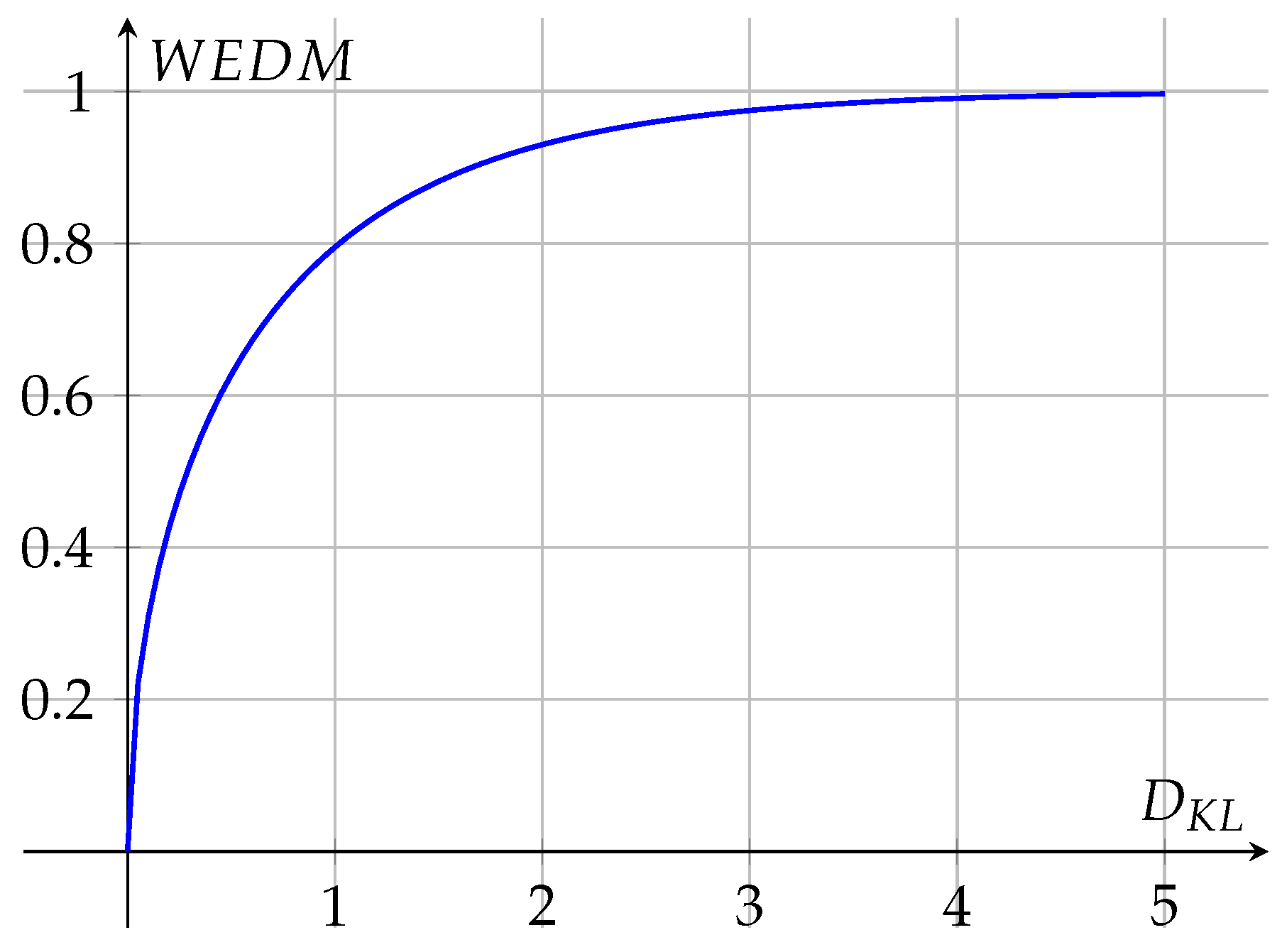
Thanks to Equation (14), we can introduce the wavelet energy divergence measure ($WEDM$), which measures how informative one series is about another. Specifically, it is defined as follows: given two signals x and y, both in $L^2\left(\mathbb{R}\right)$, the $WEDM$ of a signal x, given a signal y, is defined as

$$WEDM(x,y)=\sqrt{1-e^{-D_{KL}\left(x\right|y)}}.$$

(15)

This results in a strictly concave and increasing function of $D_{KL}\left(x\right|y)$, as can also be seen in Figure 3. For further details, see [38].

In particular, the data predictability measure has the following properties:

• If x is a deterministic function of y, knowing y reduces the uncertainty about x, enhancing its intrinsic predictability and making $WEDM$ approach zero.
• If x is unpredictable given y, its intrinsic predictability is low, and $WEDM$ nears unity.

5. Wavelet Coherence Analysis

In this section, we will analyze the time–frequency domain correlations between the considered commodities and indices. The analysis of these correlations will provide a better overview for interpreting the results of the series’ predictability and subsequent forecasting.

5.1. Wavelet Coherence of Palladium vs. Indices

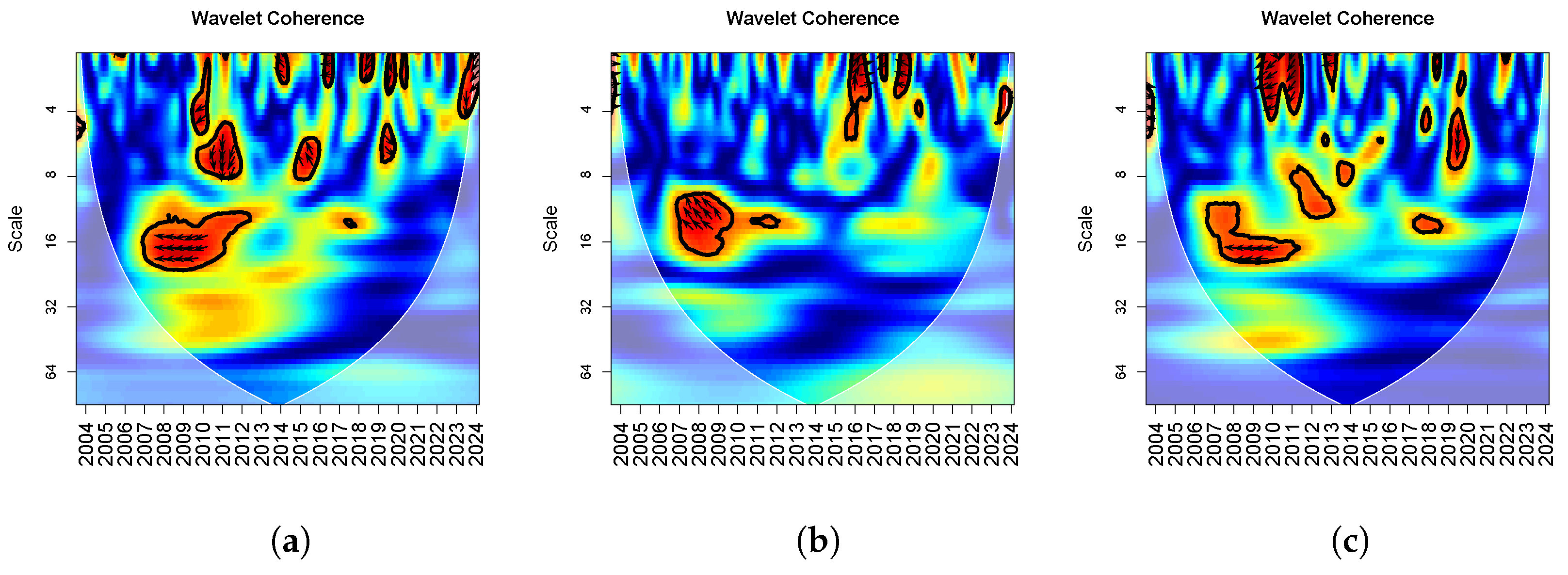
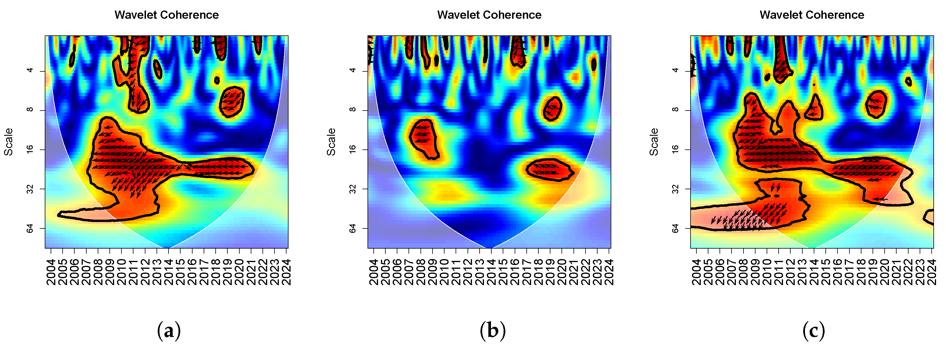
Let us now analyze the correlations between palladium and the considered indices shown in Figure 4. Tick marks are placed at July of each year to provide consistent annual reference points along the time axis. When analyzing the VIX and palladium (Figure 4a), we can observe a strong correlation in the period 2008–2013 at intermediate scales; there is no lead–lag relationship between the two series, but their movements are negatively correlated. At lower scales, meaning in the short term, we notice that throughout the analyzed time frame, the two series exhibit many correlations that are generally out of phase. In particular, in the periods 2010–2012 and 2015–2016, their movements are generally negatively correlated, with the VIX initially leading palladium and then the opposite happening, while in 2020, palladium leads the VIX. In the very short term, there are many scattered and brief correlations, which are mostly out of phase.

Regarding the STLFSI and palladium (see Figure 4c), we can observe a similar behavior to that seen with the VIX. However, the main correlations that emerge from the graph show that they always move in a negatively correlated fashion, and when a lead–lag relationship can be defined, it is generally the STLFSI that leads palladium.

The relationship between the EPUI and palladium illustrated in Figure 4b appears strong in the medium term, between 2006 and 2010, when palladium leads the EPUI, and the two series move in a negatively correlated manner. Other shorter correlations can be found in the very short term, concentrated between 2016 and 2019, where they first move in a positively correlated manner, with the EPUI leading palladium, and then move in a negatively correlated manner, with palladium leading the EPUI.

5.2. Wavelet Coherence of Heating Oil vs. Indices

Next, we examined the correlations between heating oil and the indices used, as depicted in Figure 5. When we analyzed heating oil and the VIX and heating oil and the STLFSI (see Figure 5a,c), we noticed that their correlation periods and scales are very similar. Except for at very large scales, between 2008 and 2012, where the series move in-phase and the heating oil leads both indices, in all other cases, the series move in a negatively correlated manner, with the indices tend to lead the heating oil. The strongest correlations, besides the one already mentioned, are observed at intermediate scales between 2006 and 2013, in 2015–2016, and at smaller scales (short-term) between 2018 and 2020. Other brief correlations can be observed in the very short term.

Analyzing the correlations between the EPUI and heating oil, presented in Figure 5b, we can observe similar structures, but they are less persistent over time. Notably, during the periods 2007–2010, 2018–2020, and 2022, heating oil leads the EPUI, whereas in the other two previously mentioned cases, the indices almost always lead the commodity.

5.3. Wavelet Coherence of Copper vs. Indices

Finally, let us explore the correlations between copper and the considered indices depicted in Figure 6. When analyzing the VIX and copper (see Figure 6a, we observe a strong correlation, particularly at medium to large scales, indicating a medium- to long-term relationship. This correlation is evident throughout almost the entire analyzed time frame and has a a negative comovement, meaning that when one increases, the other decreases. Additionally, there is a lead–lag relationship, where the VIX leads the copper’s futures price. In the short term, the most significant correlations appear in the 2010–2012 and 2018–2020 periods, where the two series again exhibit a negative comovement, with the VIX leading copper.

For the STLFSI and copper, as seen in Figure 6c, we also observe a strong correlation over the analyzed time frame at medium to large scales, meaning in the medium and long term. Here, the two series exhibit a negative comovement, and a lead–lag relationship emerges, with the STLFSI leading copper. The correlation is also noticeable at lower scales (in the short term) but is mainly concentrated to within 2011–2012, where the STLFSI leads copper with a negative comovement. In 2019 and early 2020, the negative comovement persists, but copper leads the STLFSI.

Rather different behavior is observed when analyzing the EPUI and copper (Figure 6b). In this case, a correlation between the two is present but much weaker. Specifically, the correlation is concentrated in certain periods that cover the medium and long term, namely 2008–2009 and late 2017–2021. In the first period, the EPUI leads copper, whereas in the second period copper leads the EPUI. Regarding a long-term trend, there are short and scattered correlations throughout the entire analyzed period, where, in some cases, it is not possible to determine a lead–lag relationship, while in others the two series exhibit both negative and positive comovements.

6. Time Series Predictability

In this section, we examine the predictability of the series using the wavelet Kullback–Leibler divergence measure, aiming to identify which of the three indices contributes the most to reducing uncertainty and consequently improving the future forecasting of commodities.

6.1. Assessing Time Series Predictability Using Kullback–Leibler Divergence

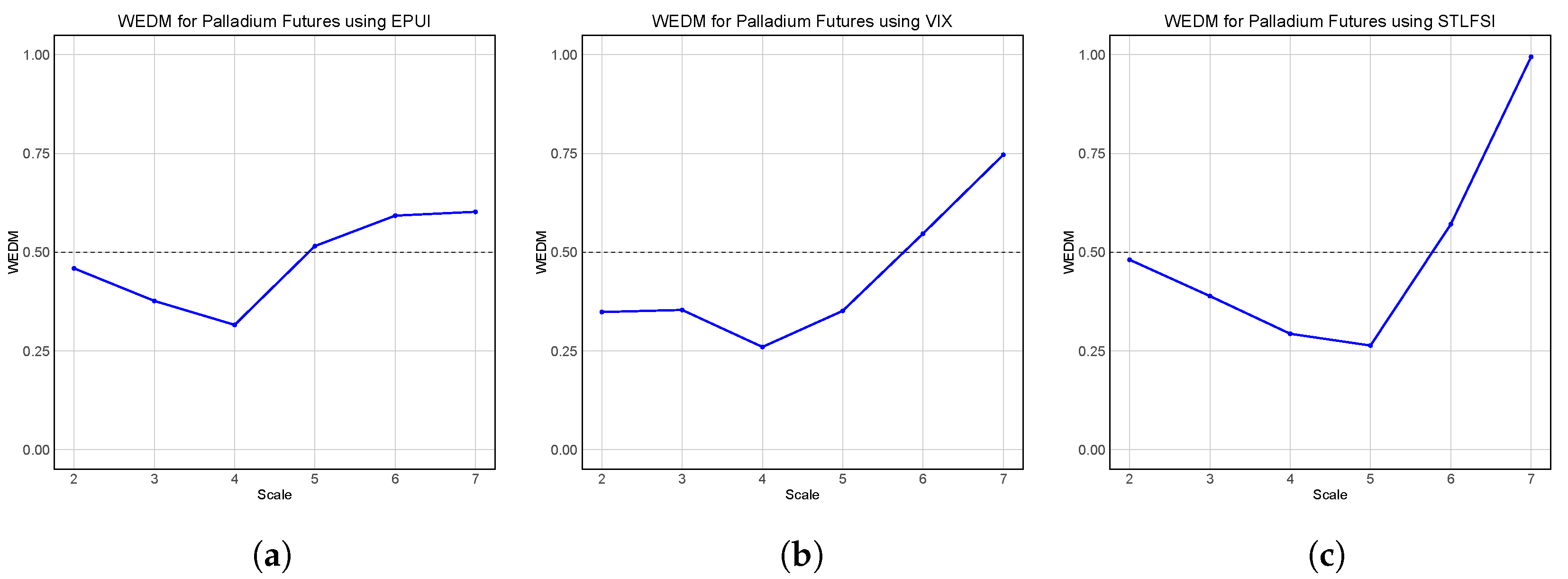
In terms of palladium’s futures price, from Figure 7, it is evident that the Economic Policy Uncertainty Index (Figure 7a) generally exhibits WEDM values that remain below or only slightly exceed 0.5 across different scales. This suggests that the EPUI has a relatively strong predictive capability for palladium’s futures price, as lower WEDM values indicate greater informativeness. While the EPUI does not always have the lowest WEDM values at every scale, it remains within a range that suggests it retains useful predictive power across both short-term and long-term fluctuations.

In contrast, the VIX index (Figure 7b) leads to WEDM values that fluctuate more across scales. While the VIX exhibits values comparable to the EPUI in some cases, at higher scales it tends to rise more significantly, reaching approximately 0.75.

The STLFSI (Figure 7c), on the other hand, displays the highest WEDM value of 0.995 at the largest scale.

These findings highlight that the EPUI provides the most stable predictive power, with WEDM values generally below 0.5.

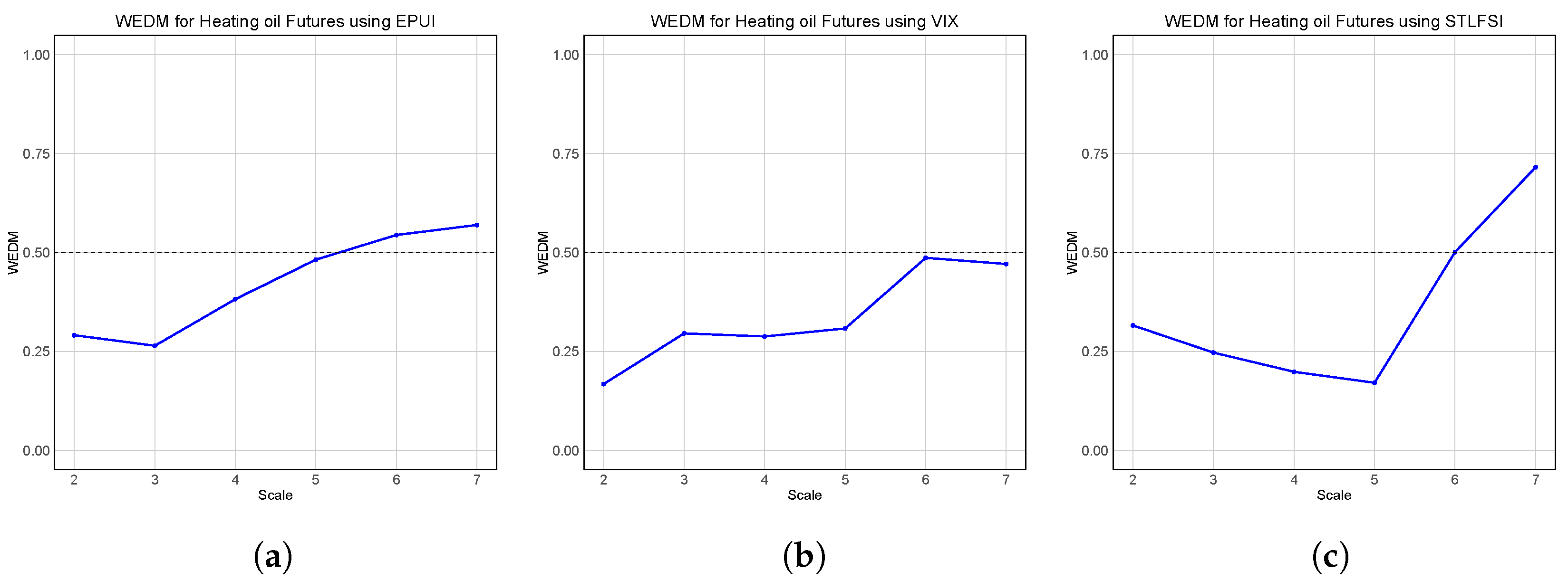
Considering the futures price of heating oil, from Figure 8 it is clear that the Economic Policy Uncertainty Index (Figure 8a) exhibits a clear upward trend, with WEDM values starting below 0.5 but progressively increasing as the scale becomes larger. Around a scale of 5, the EPUI crosses the 0.5 threshold, indicating that while it provides some predictability in the short run, its informativeness declines in the long run.

The VIX (Figure 8b) generally maintains lower WEDM values across all scales, staying close to or below 0.5. This suggests that the VIX is the most informative index for predicting heating oil’s futures price, as lower WEDM values indicate greater predictability. Even at the highest scales, the VIX does not exceed 0.5, reinforcing its role as a useful indicator of heating oil price movements.

In contrast, the STLFSI (Figure 8c) initially has lower WEDM values, similar to the VIX, but these increase rapidly after scale 5, reaching values close to 0.75 at the largest scale. This suggests that financial stress is a weak predictor of heating oil’s futures price, particularly in the long run. While the STLFSI shows some informativeness at short scales, it loses its predictive ability at larger scales.

These results highlight that the VIX is the strongest predictor of heating oil’s futures prices, as it consistently maintains lower WEDM values across all scales. The EPUI provides some predictability but weakens at larger scales, while the STLFSI is the least useful, particularly for long-term price movements, where its WEDM values rise significantly.

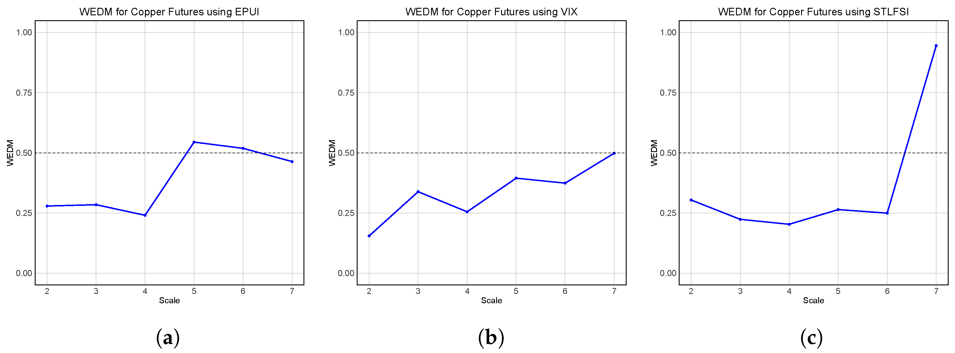
In terms of the futures price of copper, from Figure 9 it is clear that the Economic Policy Uncertainty Index (Figure 9a) initially maintains relatively low WEDM values, indicating a stronger predictive ability at smaller scales. However, at scale 5, its WEDM values rise above 0.5 and then decrease slightly further at scales above that.

The VIX (Figure 9b) displays steadily increasing WEDM values, which start low and approach 0.5 at the largest scale. This suggests that market volatility contributes significantly to the predictability of copper futures, with its strongest influence at smaller scales.

The STLFSI (Figure 9c) exhibits a distinct pattern, where its WEDM values remain low at smaller scales but increase sharply after scale 6, reaching values close to 1. This indicates that financial stress has little to no predictive power for copper futures in the long run, as high WEDM values suggest weak explanatory ability. However, for scales 3–6, the EPUI exhibits the lowest WEDM values, indicating that it has the strongest predictive power for copper’s futures prices in this range. Its relatively low values at small scales imply that the STLFSI may still have some relevance in terms of predicting short-term copper price movements, even though it loses significance over longer time horizons.

We can draw a parallel between these results and the wavelet coherence analysis from Section 5, which explored the relationships between palladium and the financial indices studied. While coherence identifies correlations across time scales, WEDM measures predictive power, offering a distinct perspective. The EPUI emerges as the most stable predictor of palladium, maintaining low WEDM values, aligning with its medium-term coherence, where palladium led the EPUI. The VIX shows fluctuating predictability, reflecting its unstable, short-term correlations. Despite the STLFSI exhibiting persistent negative coherence with palladium, its high WEDM values indicate a weak forecasting ability, reinforcing the notion that correlation does not always imply predictability.

A similar pattern emerges for heating oil, where coherence shows that the VIX and STLFSI are often negatively correlated with heating oil, with both indices leading at various scales. However, WEDM confirms that the VIX is the strongest predictor, as it maintains lower values across scales, while the EPUI declines in informativeness at larger scales. The STLFSI, though correlated with heating oil prices, exhibits high WEDM values, confirming its limited role in price forecasting. This contrast highlights how WEDM and coherence capture different aspects of the relationship—correlation does not necessarily translate to predictive power.

For copper, the coherence analysis revealed persistent negative comovements with the VIX and STLFSI, with the VIX generally leading copper. The WEDM results support this, showing that the VIX is the most informative predictor at small scales, though its influence weakens over time. The STLFSI, despite its strong coherence, has high WEDM values at larger scales, confirming its weak predictive ability. The EPUI, which showed only sporadic coherence with copper, provides the lowest WEDM values at medium scales, suggesting some predictive relevance in the medium term. These findings reinforce the need to consider both measures—coherence for relationships and WEDM for forecasting power—when analyzing financial dependencies.

6.2. Forecast

In order to assess the true predictive contribution of these financial and economic uncertainty indices, we adopted an out-of-sample forecasting approach. Specifically, the last 12 months of each commodity time series were excluded from model training. Then, Long Short-Term Memory (LSTM) models were trained on the earlier portion of the data, incorporating the indices as input features, and used to predict commodity prices in the withheld period. This setup ensures that the evaluation metrics reflect the forecasting performance of the indices on unseen data, thereby avoiding data leakage and inflated accuracy.

During the 12-month out-of-sample forecasting period, the values of the uncertainty indices were treated as known. This setting creates a conditional forecasting framework, where the goal is to evaluate the incremental predictive value of the indices for commodity price forecasting. The assumption of known inputs allows us to isolate and quantify the impact of these financial indicators, independent of any forecast error in the regressors themselves. The training set spans from January 2004 to September 2023, and the forecast period is from October 2023 to September 2024.

LSTM is a specialized type of recurrent neural network that employs gradient descent algorithms. Unlike traditional multilayer perceptrons, LSTMs use unique processing elements or blocks designed to capture long-term dependencies, making them especially suitable for time series data [40].

First, the input data needed to be rescaled to match the range of the activation function. Since the default activation function for LSTM is a hyperbolic tangent function, which maps the input values to the range $\left[-1,1\right]$, we normalized the data considering the minimum and maximum of the training data set. The predicted values were then reverted to the original scale for interpretability.

We made predictions of the commodities’ futures prices using the three analyzed indices as regressors. We used sequences of 6 months and the real indices’ values for the last 12 months to apply LSTM with a regressor.

To prevent overfitting, dropout regularization was applied to the LSTM layers. After testing various configurations, we selected dropout values of 0.4–0.5, which offered the best trade-off between bias and variance. This range aligns with recommendations from [41], who originally introduced the dropout method.

We use the following three architectures of LSTM:

• For palladium, we used 3 neurons and a dropout value of 0.5 to address overfitting.
• For heating oil, we used 10 neurons and a dropout value of 0.4 to prevent overfitting.
• For copper, we used a model with two LSTM layers, the first with 100 neurons and the second with 50 neurons, both with dropout levels of 0.4. This more complex architecture is necessary due to the significant challenges in forecasting copper prices, which exhibit high volatility and bubble-like patterns, characterized by frequent swings and speculative spikes.

The number of neurons and layers in each LSTM model was chosen manually based on exploratory testing and the complexity of the commodity’s price behavior. This approach aligns with the recommendation of [42], who argue that for problems where performance is highly data-dependent, heuristic or randomized strategies are often more effective than exhaustive grid searches. For instance, copper’s more irregular dynamics and higher volatility warranted a deeper two-layer architecture (100 and 50 neurons), while simpler configurations were sufficient for palladium and heating oil.

A linear output layer activation function was applied in all cases to ensure the predictions aligned with the continuous nature of the target variables. To avoid unnecessarily long training times, we implemented an early stopping mechanism during training [43]. Specifically, training was halted if the model’s loss did not improve for 20 consecutive epochs (a patience of 20), and the model was restored to the best-performing version based on its training loss. For all cases, we used a maximum of 800 epochs and relied on the training loss to preserve the full training set.

For each forecasted period, we calculated a Root Mean Square Error (see

Table 1. RMSE values of one-year predictions.

Model	Palladium	Heating Oil	Copper
With EPUI	55.2722	0.1604	0.4224
With VIX	62.4550	0.1565	0.4971
With STLFSI	70.8061	0.1855	0.2430

) and we found that when forecasting palladium prices, incorporating the EPUI (Economic Policy Uncertainty Index) returned the best prediction accuracy, as reflected by its lower RMSE of 55.27 compared to the accuracy measures achieved when using the other indices. This suggests that economic policy uncertainty has a meaningful relationship to palladium price movements. In fact, including the VIX (Volatility Index) or STLFSI (St. Louis Fed Financial Stress Index) worsens the forecast, leading to RMSE values of 62.46 and 70.81, respectively. Of the three indices, the EPUI is the most useful for enhancing palladium price predictions.

The corresponding forecasts are illustrated in Figure 10.

For heating oil (see Figure 11), both the EPUI and VIX lead to comparable errors of around 0.16, with the VIX returning a slightly lower RMSE of 0.1565. On the other hand, incorporating the STLFSI results in a higher RMSE of 0.19, indicating a weaker connection between financial stress and heating oil prices.

For copper prices, incorporating the STLFSI yields the most accurate forecasts, with an RMSE of 0.24. This result highlights the significant role financial stress plays in influencing copper prices. This can clearly be observed in Figure 12 where, in comparison to the other indices, only the forecasts using the STLFSI follow the increasing trend seen in the actual prices in the prediction period. Conversely, including the EPUI or VIX increases the RMSE to 0.42 or 0.50, respectively, indicating that these indices do not contribute as effectively to forecasting copper prices. Among the indices, the STLFSI is the most impactful for improving copper price predictions.

Each commodity’s relationship with the indices varies. Palladium benefits the most from incorporating the EPUI, while heating oil is best predicted when using the VIX and copper forecasts are most accurate with the STLFSI. This variability underscores the importance of tailoring predictive models to the specific characteristics of each commodity.

To enhance the interpretability of the models’ forecasting performance across commodities, we have also reported the Mean Absolute Percentage Error (MAPE) in

Table 2. MAPE values of one-year predictions.

Model	Palladium	Heating Oil	Copper
With EPUI	0.0555	0.0627	0.1021
With VIX	0.0627	0.0612	0.1201
With STLFSI	0.0711	0.0726	0.0587

. Unlike the RMSE, which reflects the magnitude of the prediction errors in the original units of each series, the MAPE expresses forecast accuracy as a percentage, allowing comparisons across time series of different scales. This additional metric provides a scale-invariant view of performance and is especially useful in assessing practical forecasting utility [44]. The reported MAPE values confirm the RMSE-based findings, with the best-performing models for each commodity also exhibiting the lowest percentage errors.

7. Conclusions

This study explored the predictability of the futures prices of commodities—palladium, heating oil, and copper—using financial and uncertainty indices assessed through wavelet coherence analysis, the wavelet Kullback–Leibler divergence measure, and LSTM forecasting models. Our findings reveal that the predictive power of each index varies across commodities, with the EPUI enhancing palladium forecasts, the VIX providing the strongest signals for heating oil, and the STLFSI being the most relevant for copper prices.

While wavelet coherence analysis identifies time-dependent correlations between commodity prices and financial indices, WEDM quantifies their predictive strength, offering a distinct perspective. In some cases, coherence and predictability align—such as with the EPUI’s influence on palladium and the VIX’s role in heating oil forecasting—but in others, strong coherence does not translate into effective prediction, as seen with the STLFSI and copper. This highlights the importance of considering both measures when assessing financial dependencies, as correlation at different time scales does not necessarily imply a strong forecasting power.

A key contribution of this study is the integration of time–frequency information and deep learning for financial time series forecasting, demonstrating that combining wavelet-based divergence measures with machine learning techniques improves our understanding of how macroeconomic uncertainty, financial stress, and market volatility affect commodity prices. Our results emphasize the necessity of tailored predictive models, as different commodities respond differently to the same financial conditions.

Despite these insights, forecasting remains particularly challenging for highly volatile assets such as copper, where only the STLFSI helped stabilize predictions. Future research should explore the nonlinear interactions between economic indicators, refine machine learning architectures for improved forecasting performance, and incorporate additional macroeconomic drivers to enhance predictability. By bridging wavelet-based uncertainty quantification with data-driven forecasting, this study provides a novel approach to understanding financial dependencies in commodity markets.

References

- Williams, J.R.; Amaratunga, K. Introduction to wavelets in engineering. Int. J. Numer. Methods Eng. 1994, 37, 2365–2388. [Google Scholar] [CrossRef]
- Sarkar, T.K.; Salazar-Palma, M.; Wicks, M.C. Wavelet Applications in Engineering Electromagnetics; Artech House: Norwood, MA, USA, 2002. [Google Scholar]
- Mazzoccoli, A.; Rivero, J.A.; Vellucci, P. Refining Heisenberg’s principle: A greedy approximation of step functions with triangular waveform dictionaries. Math. Comput. Simul. 2024, 225, 165–176. [Google Scholar] [CrossRef]
- Mastroeni, L.; Mazzoccoli, A.; Quaresima, G. Effects of the climate-related sentiment on agricultural spot prices: Insights from Wavelet Rényi Entropy analysis. Energy Econ. 2025, 142, 108146. [Google Scholar] [CrossRef]
- Antoniadis, A. Wavelets in statistics: A review. J. Ital. Stat. Soc. 1997, 6, 97–130. [Google Scholar] [CrossRef]
- Vidakovic, B. Statistical Modeling by Wavelets; John Wiley & Sons: Hoboken, NJ, USA, 2009. [Google Scholar]
- Bilgili, F.; Koçak, E.; Kuşkaya, S.; Bulut, Ü. Estimation of the co-movements between biofuel production and food prices: A wavelet-based analysis. Energy 2020, 213, 118777. [Google Scholar] [CrossRef]
- Zheng, B.; Zhang, Y.W.; Qu, F.; Geng, Y.; Yu, H. Do rare earths drive volatility spillover in crude oil, renewable energy, and high-technology markets?—A wavelet-based BEKK- GARCH-X approach. Energy 2022, 251, 123951. [Google Scholar] [CrossRef]
- Zhu, P.; Tang, Y.; Wei, Y.; Dai, Y.; Lu, T. Relationships and portfolios between oil and Chinese stock sectors: A study based on wavelet denoising-higher moments perspective. Energy 2021, 217, 119416. [Google Scholar] [CrossRef]
- Aguiar-Conraria, L.; Soares, M.J. The continuous wavelet transform: Moving beyond uni- and bivariate analysis. J. Econ. Surv. 2014, 28, 344–375. [Google Scholar] [CrossRef]
- Mastroeni, L.; Mazzoccoli, A.; Quaresima, G.; Vellucci, P. Wavelet analysis and energy-based measures for oil-food price relationship as a footprint of financialisation effect. Resour. Policy 2022, 77, 102692. [Google Scholar] [CrossRef]
- Cheung, C.S.; Miu, P. Diversification benefits of commodity futures. J. Int. Financ. Mark. Institutions Money 2010, 20, 451–474. [Google Scholar] [CrossRef]
- Silvennoinen, A.; Thorp, S. Financialization, crisis and commodity correlation dynamics. J. Int. Financ. Mark. Inst. Money 2013, 24, 42–65. [Google Scholar] [CrossRef]
- Hammoudeh, S.; Nguyen, D.K.; Reboredo, J.C.; Wen, X. Dependence of stock and commodity futures markets in China: Implications for portfolio investment. Emerg. Mark. Rev. 2014, 21, 183–200. [Google Scholar] [CrossRef]
- Pastor, L.; Veronesi, P. Uncertainty about government policy and stock prices. J. Financ. 2012, 67, 1219–1264. [Google Scholar] [CrossRef]
- Reboredo, J.C.; Wen, X. Are China’s new energy stock prices driven by new energy policies? Renew. Sustain. Energy Rev. 2015, 45, 624–636. [Google Scholar] [CrossRef]
- Wang, Y.; Zhang, B.; Diao, X.; Wu, C. Commodity price changes and the predictability of economic policy uncertainty. Econ. Lett. 2015, 127, 39–42. [Google Scholar] [CrossRef]
- Yin, L.; Han, L. Macroeconomic uncertainty: Does it matter for commodity prices? Appl. Econ. Lett. 2014, 21, 711–716. [Google Scholar] [CrossRef]
- Nittayakamolphun, P.; Bejrananda, T.; Pholkerd, P. Asymmetric Effects of Uncertainty and Commodity Markets on Sustainable Stock in Seven Emerging Markets. J. Risk Financ. Manag. 2024, 17, 155. [Google Scholar] [CrossRef]
- Dovern, J.; van Roye, B. International transmission and business-cycle effects of financial stress. J. Financ. Stab. 2014, 13, 1–17. [Google Scholar] [CrossRef]
- Cheng, I.H.; Kirilenko, A.; Xiong, W. Convective risk flows in commodity futures markets. Rev. Financ. 2015, 19, 1733–1781. [Google Scholar] [CrossRef]
- Bakas, D.; Triantafyllou, A. Commodity price volatility and the economic uncertainty of pandemics. Econ. Lett. 2020, 193, 109283. [Google Scholar] [CrossRef]
- Nazlioglu, S.; Soytas, U.; Gupta, R. Oil prices and financial stress: A volatility spillover analysis. Energy Policy 2015, 82, 278–288. [Google Scholar] [CrossRef]
- Adhikari, R.; Putnam, K.J. Macroeconomic Conditions, Speculation, and Commodity Futures Returns. Int. J. Financ. Stud. 2025, 13, 5. [Google Scholar] [CrossRef]
- Fama, E.F. Forward and spot exchange rates. J. Monet. Econ. 1984, 14, 319–338. [Google Scholar] [CrossRef]
- Verheyen, F. Monetary policy, commodity prices and inflation-empirical evidence from the US. In Commodity Prices and Inflation-Empirical Evidence from the US (November, 19 2010); Ruhr-Universität Bochum (RUB), Department of Economics Universitätsstr: Bochum, Germany, 2010. [Google Scholar]
- Wang, G.; Guo, L.; Duan, H. Wavelet neural network using multiple wavelet functions in target threat assessment. Sci. World J. 2013, 2013, 632437. [Google Scholar] [CrossRef] [PubMed]
- Lee, D.T.; Yamamoto, A. Wavelet analysis: Theory and applications. Hewlett Packard J. 1994, 45, 44. [Google Scholar]
- Dong, M.; Chang, C.P.; Gong, Q.; Chu, Y. Revisiting global economic activity and crude oil prices: A wavelet analysis. Econ. Model. 2019, 78, 134–149. [Google Scholar] [CrossRef]
- Aguiar-Conraria, L.; Soares, M.J. Oil and the macroeconomy: Using wavelets to analyze old issues. Empir. Econ. 2011, 40, 645–655. [Google Scholar] [CrossRef]
- Torrence, C.; Compo, G.P. A Practical Guide to Wavelet Analysis. Bull. Am. Meteorol. Soc. 1998, 79, 61–78. [Google Scholar] [CrossRef]
- Bašta, M.; Molnár, P. Oil market volatility and stock market volatility. Financ. Res. Lett. 2018, 26, 204–214. [Google Scholar] [CrossRef]
- Grinsted, A.; Moore, J.C.; Jevrejeva, S. Application of the cross wavelet transform and wavelet coherence to geophysical time series. Nonlinear Process. Geophys. 2004, 11, 561–566. [Google Scholar] [CrossRef]
- Mastroeni, L.; Mazzoccoli, A.; Vellucci, P. Wavelet entropy and complexity–entropy curves approach for energy commodity price predictability amid the transition to alternative energy sources. Chaos Solitons Fractals 2024, 184, 115005. [Google Scholar] [CrossRef]
- Maraun, D.; Kurths, J. Cross wavelet analysis: Significance testing and pitfalls. Nonlinear Process. Geophys. 2004, 11, 505–514. [Google Scholar] [CrossRef]
- Bloomfield, D.S.; McAteer, R.T.J.; Lites, B.W.; Judge, P.G.; Mathioudakis, M.; Keenan, F.P. Wavelet Phase Coherence Analysis: Application to a Quiet-Sun Magnetic Element. Astrophys. J. 2004, 617, 623–632. [Google Scholar] [CrossRef]
- Mastroeni, L.; Mazzoccoli, A.; Vellucci, P. Studying the impact of fluctuations, spikes and rare events in time series through a wavelet entropy predictability measure. Phys. A Stat. Mech. Its Appl. 2024, 641, 129720. [Google Scholar] [CrossRef]
- Mastroeni, L.; Mazzoccoli, A. Quantifying predictive knowledge: Wavelet energy α-divergence measure for time series uncertainty reduction. Chaos Solitons Fractals 2024, 188, 115488. [Google Scholar] [CrossRef]
- Nishiyama, T. Convex optimization on functionals of probability densities. arXiv 2020, arXiv:2002.06488. [Google Scholar]
- Hochreiter, S.; Schmidhuber, J. Long short-term memory. Neural Comput. 1997, 9, 1735–1780. [Google Scholar] [CrossRef]
- Srivastava, N.; Hinton, G.; Krizhevsky, A.; Sutskever, I.; Salakhutdinov, R. Dropout: A simple way to prevent neural networks from overfitting. J. Mach. Learn. Res. 2014, 15, 1929–1958. [Google Scholar]
- Bergstra, J.; Bengio, Y. Random search for hyper-parameter optimization. J. Mach. Learn. Res. 2012, 13, 281–305. [Google Scholar]
- Brownlee, J. A gentle introduction to early stopping to avoid overtraining neural networks. Mach. Learn. Mastery 2018, 7. [Google Scholar]
- Makridakis, S.; Hibon, M. Accuracy of forecasting: An empirical investigation. J. R. Stat. Soc. Ser. A (Gen.) 1979, 142, 97–125. [Google Scholar] [CrossRef]
Figure 1.
Futures prices of palladium, heating oil, and copper.
Figure 2.
EPUI, VIX, and STLFSI indices.
Figure 3.
The wavelet energy divergence measure as a function of the wavelet Kullbach–Leibler divergence.
Figure 4.
Wavelet coherence of palladium across the considered indices, the colors ranging from blue to red indicate the intensity of the correlation between the analyzed series: the closer to blue, the less correlated they are; the closer to red, the more correlated they are. (a) Wavelet coherence between palladium and the VIX. (b) Wavelet coherence between palladium and the EPUI. (c) Wavelet coherence between palladium and the STLFSI.
Figure 5.
Wavelet coherence of heating oil across the considered indices, the colors ranging from blue to red indicate the intensity of the correlation between the analyzed series: the closer to blue, the less correlated they are; the closer to red, the more correlated they are. (a) Wavelet coherence between heating oil and the VIX. (b) Wavelet coherence between heating oil and the EPUI. (c) Wavelet coherence between heating oil and the STLFSI.
Figure 6.
Wavelet coherence of copper across the considered indices, the colors ranging from blue to red indicate the intensity of the correlation between the analyzed series: the closer to blue, the less correlated they are; the closer to red, the more correlated they are. (a) Wavelet coherence between copper and the VIX. (b) Wavelet coherence between copper and the EPUI. (c) Wavelet coherence between copper and the STLFSI.
Figure 7.
Wavelet Kullback–Leibler divergence measure of palladium’s futures price across the considered indices. (a) WEDM for palladium using the EPUI. (b) WEDM for palladium using the VIX. (c) WEDM for palladium using the STLFSI.
Figure 8.
Wavelet Kullback–Leibler divergence measure of heating oil’s futures price across the considered indices. (a) WEDM for heating oil using the EPUI. (b) WEDM for heating oil using the VIX. (c) WEDM for heating oil using the STLFSI.
Figure 9.
Wavelet Kullback–Leibler divergence measure for copper’s futures price across the considered indices. (a) WEDM for copper using the EPUI. (b) WEDM for copper using the VIX. (c) WEDM for copper using the STLFSI.
Figure 10.
Palladium futures prices predicted using LSTM. The red dotted line represents the predictions. The shadowed region denotes the period covered by the forecast. (a) Forecasting palladium using the EPUI. (b) Forecasting palladium using the VIX. (c) Forecasting palladium using the STLFSI.
Figure 11.
Heating oil futures prices predicted using LSTM. The red dotted line represents the predictions. The shadowed region denotes the period covered by the forecast. (a) Forecasting heating oil using the EPUI. (b) Forecasting heating oil using the VIX. (c) Forecasting heating oil using the STLFSI.
Figure 12.
Copper futures prices predicted using LSTM. The red dotted line represents the predictions. The shadowed region denotes the period covered by the forecast. (a) Forecasting copper using the EPUI. (b) Forecasting copper using the VIX. (c) Forecasting copper using the STLFSI.