Intelligent Dynamic Multi-Dimensional Heterogeneous Resource Scheduling Optimization Strategy Based on Kubernetes

Abstract

In this paper, we tackle the challenge of optimizing resource utilization and demand-driven allocation in dynamic, multi-dimensional heterogeneous environments. Traditional containerized task scheduling systems, like Kubernetes, typically rely on default schedulers that primarily focus on CPU and memory, overlooking the multi-dimensional nature of heterogeneous resources such as GPUs, network I/O, and disk I/O. This results in suboptimal scheduling and underutilization of resources. To address this, we propose a dynamic scheduling method for heterogeneous resources using an enhanced Technique for Order Preference by Similarity to Ideal Solution (TOPSIS) algorithm that adjusts weights in real time and applies nonlinear normalization. Leveraging parallel computing, approximation, incremental computation, local updates, and hardware acceleration, the method minimizes overhead and ensures efficiency. Experimental results showed that, under low-load conditions, our method reduced task response times by 31–36%, increased throughput by 20–50%, and boosted resource utilization by over 20% compared to both the default Kubernetes scheduler and the Kubernetes Container Scheduling Strategy (KCSS) algorithm. These improvements were tested across diverse workloads, utilizing CPU, memory, GPU, and I/O resources, in a large-scale cluster environment, demonstrating the method’s robustness. These enhancements optimize cluster performance and resource efficiency, offering valuable insights for task scheduling in containerized cloud platforms.

1. Introduction

Rapid advancements in cloud computing and containerization have made Kubernetes, a leading container orchestration platform, a key component of modern application architectures [1]. However, the default Kubernetes scheduler (Kube-scheduler) primarily focuses on scheduling homogeneous resources like CPU and memory, with limited support for heterogeneous resources such as GPUs, network I/O, and disk I/O [2]. This constraint hampers the scheduler’s ability to efficiently manage complex resource demands, particularly in GPU-intensive tasks like deep learning, where the lack of fine-grained control over resource allocation can lead to inefficient utilization or over-allocation, ultimately affecting task scheduling efficiency, training performance, and overall system effectiveness [3].

Kubernetes offers limited management of network and disk I/O. While the CNI and CSI plugins provide extended support, they do not offer the same level of precision in scheduling as CPU and memory [4]. In high-throughput or low-latency scenarios, such as video streaming or large-scale databases, network and storage bottlenecks can significantly degrade performance, increasing latency or reducing throughput [5]. Google Cloud’s Kubernetes Performance Guide identifies network and disk I/O contention as a common issue in production environments, particularly in multi-tenant cloud settings, where insufficient scheduling can lead to performance instability in data-intensive applications [6].

Recent developments in Kubernetes resource scheduling, fueled by advances in cloud computing and container technologies, have made strides in overcoming these limitations. For example, Du and T. [7] introduced a distributed machine-learning-based priority scheduling method that improves scheduling efficiency by incorporating factors such as user and task priorities, waiting times, task parallelism, and node affinity. Wang [8] used deep reinforcement learning to optimize edge task scheduling, achieving a 31% reduction in average response time after deploying 500 random tasks. Chehardoli [9] proposed a dynamic network-metrics-based scheduling strategy utilizing the Istio service mesh to gather network data, which reduced response times to 37% of their original value and saved 50% of node bandwidth. Zheng and T. [10] developed an elastic resource scheduling algorithm for container clouds that maximizes resource utilization by optimizing virtual machine configurations and resource allocation. Although these studies have advanced Kubernetes scheduling, most focus on homogeneous resources, leaving the complex interdependencies of heterogeneous resources underexplored, which limits the precision of resource allocation [11].

Traditional resource scheduling methods often rely on static configurations and fail to dynamically adjust in response to fluctuating resource demands or cluster load. As a result, static approaches can lead to resource wastage or scheduling delays. Lefteris [12] improved the existing CPU and memory filtering algorithm by incorporating GPU filtering and refining the scheduler’s scoring mechanism for mixed CPU/GPU deployments, reducing resource contention. Shen [13] developed a multi-agent critic algorithm to optimize edge cloud scheduling using a graph neural network, which increased system throughput by 15.9% and reduced scheduling costs by 38.4%. Pei [14] introduced a multi-resource interleaving scheme using deep reinforcement learning to improve performance in cloud-edge systems, addressing high-throughput task scheduling needs through a dynamic task scheduling approach. However, these methods still lack a unified framework for managing multidimensional heterogeneous resource scheduling, leading to inefficiencies when coscheduling various resource types [15,16].

In conclusion, while existing scheduling algorithms are effective at managing CPU and memory resources, they often struggle to address the complexities associated with heterogeneous resources and adapt dynamically to real-time fluctuations. This leads to suboptimal scheduling and inefficient resource utilization. To overcome these limitations, we propose a dynamic scheduling method for heterogeneous resources in Kubernetes, which simultaneously considers CPU, memory, GPU, network I/O, and disk I/O. By continuously monitoring resource usage across nodes and pods, our approach can predict shifting resource demands in real time, enabling more accurate scheduling and minimizing both resource wastage and node overload.

This paper is organized as follows: Section 2 provides an overview of the research landscape in this area. Section 3 presents a detailed discussion of the proposed algorithmic improvements, emphasizing the key advancements. Section 4 outlines the experimental setup and parameters. Section 5 offers a brief summary of the algorithms introduced in this study, along with directions for future research.

2. Research Foundation

Kubernetes [17,18] is an open-source container orchestration platform designed to automate the deployment, scaling, and management of containerized applications. Its core functionalities include load balancing, resource scheduling, and cluster management, which collectively enable efficient task distribution and resource management in heterogeneous environments. Among these components, the Kube-scheduler plays a critical role in selecting the most appropriate node for a Pod based on predefined policies [19]. The scheduling process is comprised of two main phases: node filtering and optimal ranking, which together provide both flexibility and precision in resource allocation.

In the scheduling process, Kube-scheduler first filters out the eligible node set, according to the resource requirements of the task $N_f$; the filtering method is shown in Equation (1).

$${\mathbf{N}}_{\mathbf{f}}=\left\{\mathbf{n}\in \mathbb{N}\mid {\mathbf{R}}_t\le {\mathbf{R}}_n\right\}$$

(1)

where N denotes the set of all nodes, $R_t$ is the task resource demand vector, and $R_n$ is the node resource availability vector. The selected nodes select the optimal node $n^{*}$, as shown in Equation (2).

$$n^{*}=arg\underset{\begin{array}{c}n\in {\mathbf{N}}_f\end{array}}{max}S\left(n\right)$$

(2)

where $S\left(n\right)$ is the node score function. The default Kubernetes scheduler struggles to dynamically adapt to heterogeneous resource environments, particularly when faced with varying task requirements and uneven resource loads. Dynamic resource scheduling seeks to optimize resource allocation through real-time monitoring and feedback, with the goal of maximizing system throughput and minimizing task latency.

The core objective function in Equation (3) is derived from related work and serves as a conceptual guideline, not a direct part of our algorithm. It provides a theoretical foundation for balancing task latency and resource efficiency, facilitating comparison with prior research. However, it is not integrated into our design or node scoring/scheduling logic and does not influence our algorithm’s decisions.

$$min\sum _{t\in T}\left(\alpha ·{\displaystyle \frac{C_t}{Q_{t,n}}}+\beta ·L_{t,n}\right)$$

(3)

where T is the set of tasks, $c_t$ represents the resource consumption of task t, $Q_{t,n}$ is the amount of resources allocated by task t at node n, $L_{t,n}$ is the scheduling delay of the task, and $\alpha$ and $\beta$ are the weight coefficients. The default Kubernetes scheduler struggles to dynamically adapt to heterogeneous resource environments, particularly when faced with variable task requirements and uneven resource loads. Dynamic resource scheduling seeks to optimize resource allocation through real-time monitoring and feedback, with the goal of maximizing system throughput and minimizing task latency. The core objective function is formulated as shown in Equation (3).

The cumulative reward function R, defined in Equation (4), serves as a conceptual foundation for reinforcement-learning-based task scheduling. While it suggests the use of a learning-based scheduler, this study does not incorporate reinforcement learning or reward-based optimization. Instead, the function provides a theoretical reference and baseline for related algorithms. It is not part of our proposed method, which focuses on a different scheduling approach, and is included to contextualize our work within the broader research landscape.

$$R=\sum _{t=0}^T{r}^{t}reward(s_t,a_t)$$

(4)

where $\gamma$ is the discount factor, and $s_t$ and $a_t$ represent the state and action.

3. Research Method

In this section, we provide an overview of the algorithm’s framework and the underlying research principles. The section is structured into three parts: the general algorithm, the dynamic resource weight adjustment strategy, and the enhanced TOPSIS algorithm.

3.1. General Algorithm Framework

This paper introduces a dynamic, multi-dimensional, heterogeneous resource scheduling algorithm based on Kubernetes [20]. The proposed algorithm integrates a dynamic resource weight adjustment strategy and an enhanced TOPSIS algorithm for real-time node scoring and ranking, thereby enabling precise scheduling of heterogeneous tasks [21]. The algorithm evaluates the demand and load conditions of various multi-dimensional resources, adjusting the weights of each resource based on real-time data. The enhanced TOPSIS algorithm then assigns comprehensive scores to the available nodes, ensuring that tasks are prioritized and allocated to the most suitable nodes [22]. Finally, using these node scores, real-time scheduling decisions are made to optimize resource allocation, improving resource utilization and enhancing task execution efficiency.

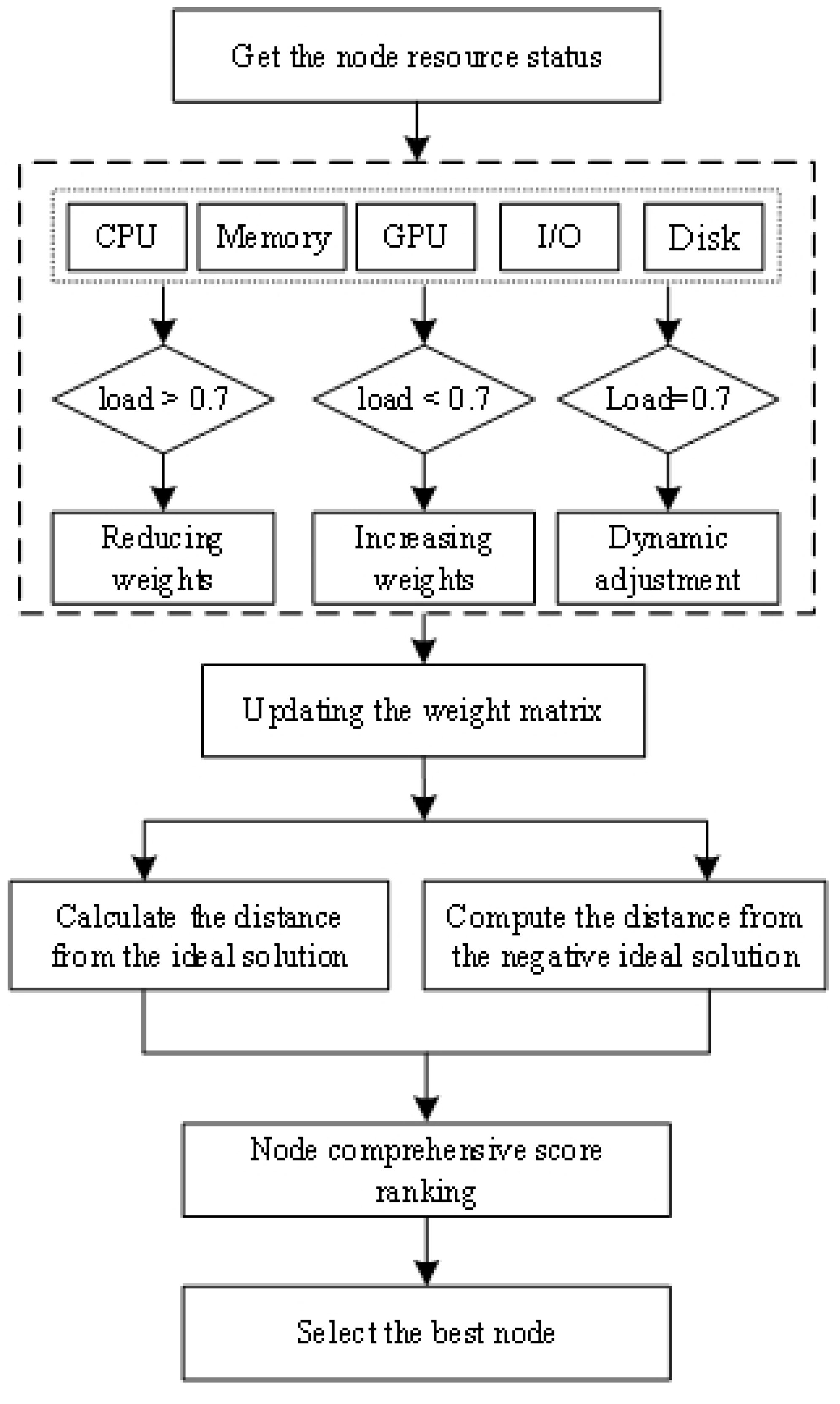
The overall workflow of the proposed algorithm is shown in Figure 1. It separates the system into three load conditions: load > 0.7, load < 0.7, and load = 0.7. The “load = 0.7” category refers to the case where the load is exactly 0.7. It acts as a boundary between the other two conditions, where the load is either greater than or less than 0.7.

As shown in Figure 1, the algorithm evaluates the demand and load of various multi-dimensional resources, adjusting the weight of each resource based on real-time data. Once the weight matrix has been updated, the output is divided into two components to assess the relative proximity of the available nodes to both the ideal and negative ideal solutions. This division is a crucial feature of the modified TOPSIS algorithm, which first calculates the distance to the ideal solution and then to the negative ideal solution.

The distance from the ideal solution path measures how closely each node approaches the best performance across all criteria, while the distance from the negative ideal solution path quantifies how far each node is from the worst-case scenario. By evaluating these distances, the algorithm ranks nodes based on their proximity to both the ideal and negative ideal solutions, ensuring tasks are allocated to the most optimal nodes. The modified TOPSIS algorithm then assigns scores to nodes, prioritizing tasks and making real-time scheduling decisions to optimize resource utilization and improve system performance.

3.2. Dynamic Resource Weight Adjustment Strategy

To achieve accurate task scheduling in heterogeneous environments, it is essential to adjust resource weights based on their real-time status and task demands [23]. We propose a dynamic weight adjustment strategy that prioritizes resources according to task requirements: for CPU- and memory-intensive tasks, CPU and memory resources are given higher weights; for GPU- and I/O-intensive tasks, GPU resources are prioritized; and for disk-intensive tasks, disk weights are adjusted to optimize storage and I/O performance [24].

The core of this strategy is the real-time modulation of resource importance, driven by cluster load and task needs [25]. The system continuously monitors resource usage and updates weights to ensure critical resources are prioritized. These adjustments occur dynamically in response to fluctuations in workload and resource availability, with more frequent updates in fluctuating environments and less frequent updates in stable ones. This adaptive approach enhances resource utilization and minimizes waste, making it effective in diverse settings such as mixed workloads or dynamic cloud environments [26].

The system considers factors such as task characteristics, node resource status, and current load, dynamically adjusting the resource weights using the following Formula (5).

$$W_{r_j}\left(t\right)={\displaystyle \frac{w_{r_j}^0}{1+a\left|R_{r_j}\left(t\right)-T_{r_j}\right|}}$$

(5)

where $W_{r_j}\left(t\right)$ is for dynamically adjusting the weight of the resource, $w_{r_j}^0$ is the initial weight of the resource dimension, $R_{r_j}\left(t\right)$ is the current resource state of the node on $r_j$, $T_{r_j}$ is the requirement of task T on $r_j$, and $\alpha$ is an adjustment coefficient that controls the degree of influence of resource state differences on weight adjustment.

To ensure that the weight sum of all resource dimensions is one, the adjusted weights need to be normalized, and the normalized weight calculation $w_{r_j}^{\prime }\left(t\right)$ is shown in Equation (6).

$$w_{r_j}^{\prime }\left(t\right)={\displaystyle \frac{w_{r_j}\left(t\right)}{{\sum }_{j=1}^n{w}_{r_j}\left(t\right)}}$$

(6)

The detailed dynamic resource weight control retuning policy is as follows.

The primary goal of Algorithm 1 is to ensure that resource allocation is closely aligned with the specific requirements of the current task, while still maintaining the load-balancing policy. The dynamic weight modulation based on load thresholds (Lines 3–7) prioritizes the use of underutilized resources and helps prevent the overloading of already stressed resources. However, once these load-balancing adjustments have been made, it is crucial to incorporate the task-specific resource requirements into line 8 to ensure that the most suitable resources are assigned to the task. This design does not override the load-balancing mechanism; instead, it enhances it by better aligning resource allocation with the real-time demands of the tasks. By combining dynamic load adjustment with task-specific resource needs, the algorithm achieves a balance between optimal task allocation and overall cluster load balancing.

Algorithm 1: Dynamic resource weight adjustment strategy

Input: Task type T; Cluster load L

Output: The adjusted resource weight W

1. W = {GPU: 1.0, CPU: 1.0, Memory: 1.0, Network: 1.0, Storage: 1.0}

2. for each R in W

3. if L[R] > 0.7

4. $W{\left[R\right]}^{*}=0.8$ // Decrease weight for heavily utilized resources

5. else if L[R] < 0.3

6. $W{\left[R\right]}^{*}=1.2$ // Increase weight for underutilized resources

7. end if

8. $W{\left[R\right]}^{*}=\mathrm{task\_need}\left[R\right]$ // Adjust weight based on task needs for resource R

9. end for

10. ${\mathit{W}}_{\mathrm{total}}$ = sum(W.values()) // Calculate the total weight of all resources

11. For each R in W

12. W[R]/ = ${\mathit{W}}_{\mathrm{total}}$ // Normalize weights based on the total weight

13. end for

3.3. Improved TOPSIS Algorithm

To effectively address the multi-dimensional heterogeneous resource scheduling problem, task scheduling must consider not only the availability of resources but also the performance of each node across various resource dimensions [27]. To this end, we propose an enhanced TOPSIS algorithm, termed Dynamic TOPSIS (D-TOPSIS), which performs comprehensive node scoring and ranking to enable precise resource scheduling. The algorithm evaluates the relative proximity of each node to the ideal solution by simultaneously factoring in resource availability and task requirements [28]. Based on this evaluation, a scheduling priority is assigned to each node. The specific steps of the D-TOPSIS algorithm are outlined as follows.

According to the resource status of each node in the different resource dimensions, decision Matrix $X=\left[x_{ij}\right]$ is constructed, as shown in Equation (7). There are m nodes and n resource dimensions. The decision matrix is $m\times n$.

$$\mathbf{X}=\left[\begin{array}{cccc}{x}_{11}& x_{12}& \cdots & x_{1n}\\ x_{21}& x_{22}& \cdots & x_{2n}\\ ⋮& ⋮& \ddots & ⋮\\ x_{m1}& x_{m2}& \cdots & x_{mn}\end{array}\right]$$

(7)

where $X=\left[x_{ij}\right]$ denotes the performance index of the i node in the j resource dimension. Since the units of different resource dimensions vary, the decision matrix must be normalized to ensure comparability across dimensions and eliminate dimensional effects. The normalization formula is given in Equation (8).

$$r_{ij}={\displaystyle \frac{x_{ij}}{\sqrt{{\sum }_{i=1}^m{x}_{ij}^2}}}$$

(8)

where $X=\left[r_{ij}\right]$ is the normalized decision matrix element and represents the normalized value of node i in resource dimension j. As per the dynamic resource weight adjustment strategy outlined in the previous section, the resource weights will be dynamically updated based on the current conditions during the scheduling process. Consequently, the weight of each resource dimension will vary at different time points. The formula for calculating the weighted normalized value $r_{ij}^{\prime }$ is shown in Equation (9).

$$r_{ij}^{\prime }=w_j·r_{ij}$$

(9)

where $w_j$ is the weight j of the resource dimension. Using the weighted normalized decision matrix, the performance of each node across all resource dimensions can be evaluated. The ideal and negative ideal solutions correspond to the best and worst node performances in each resource dimension. The definitions of ideal solutions $A^{+}$ and negative ideal solutions $A^{-}$ are given in Equation (10).

$$\begin{array}{c}\hfill A^{+}=\left(max\left(r_{1j}^{\prime },r_{2j}^{\prime },\cdots ,r_{mj}^{\prime }\right)\right)\\ \hfill A^{-}=\left(min\left(r_{1j}^{\prime },r_{2j}^{\prime },\cdots ,r_{mj}^{\prime }\right)\right)\end{array}$$

(10)

Here, $A^{+}$ and $A^{-}$ represent the maximum and minimum values for each resource dimension among all nodes. The performance of a node can be quantified by calculating the Euclidean distance between each node and both the ideal and negative ideal solutions, as expressed in Equation (11).

$$\begin{array}{c}\hfill D_i^{+}=\sqrt{\sum _{j=1}^n{\left(r_{ij}^{\prime }-A_j^{+}\right)}^2}\\ \hfill D_i^{-}=\sqrt{\sum _{j=1}^n{\left(r_{ij}^{\prime }-A_j^{-}\right)}^2}\end{array}$$

(11)

where $D_i^{+}$ and $D_i^{-}$ are the distances of nodes to ideal and negative ideal solutions. Then, the distance is used to calculate the relative proximity of each node $C_i$, which is the ratio of the distance from the node to the ideal solution and the total distance from the ideal solution and the negative ideal solution. The calculation formula is shown in Equation (12).

$$C_i={\displaystyle \frac{D_i^{-}}{D_i^{-}+D_i^{+}}}$$

(12)

where $C_i$ is the proximity of a node i, where a value closer to one indicates that the node is better, and a value closer to zero indicates that the node is worse. Finally, the nodes are ranked based on their relative proximity, with nodes exhibiting higher proximity prioritized as scheduling targets. The task is then scheduled to the node with the highest score. The steps of the improved TOPSIS algorithm are outlined below (Algorithm 2).

The D-TOPSIS algorithm enhances the traditional TOPSIS method to address resource scheduling challenges in heterogeneous environments, focusing on dynamic decision-making and adaptability to fluctuating resource demands. It introduces nonlinear normalization to preserve resource data diversity, ensuring accurate evaluations in variable environments. Dynamic weight adjustment adapts the importance of resource types based on real-time data, overcoming static weights. Real-time node scoring and ranking enable dynamic assessment and optimal task–node assignment.

Algorithm 2: The modified TOPSIS algorithm.

Input: Resource matrix R

Output: Best node

1. For each node i in R:

2. ${.\mathrm{mark}}_i=\mathrm{Standardize}\left(R_i\right)$

3. end for

4. $\mathrm{IdealSolution}\leftarrow max(R,\mathrm{axis}=0)$

5. $\mathrm{NegativeIdealSolution}\leftarrow min(R,\mathrm{axis}=0)$

6. for iter = 1 to MaxIter

7. $\mathrm{MatchDegree}\leftarrow (R,T)$

8. $W\leftarrow \mathrm{MatchDegree}$

9. $\mathrm{if}\parallel W_{\mathrm{new}}-W_{\mathrm{old}}\parallel <ϵ$

10. break

11. end for

12. for i = 1 to n

13. $D_i^{+}\leftarrow \mathrm{EuclideanDistance}(R_i,\mathrm{IdealSolution})$

14. $D_i^{-}\leftarrow \mathrm{EuclideanDistance}(R_i,\mathrm{NegativeIdealSolution})$

15. $S_i\leftarrow {\displaystyle \frac{D_i^{-}}{D_i^{+}+D_i^{-}}}$

16. end for

17. $S_{\mathrm{sorted}}\leftarrow \mathrm{Sort}\left(S\right)$

18. $\mathrm{Best\_node}\leftarrow S_{\mathrm{sorted}}\left[0\right]$

While these improvements enhance scheduling accuracy, they also introduce computational overhead due to dynamic weight adjustments and real-time scoring. To address this, we utilize parallel computing, enabling simultaneous processing of node evaluations and weight adjustments across multiple cores or systems, thereby reducing computation time. Approximation techniques strike a balance between speed and accuracy, allowing for the efficient handling of large datasets. Incremental computation ensures that only the affected parts of the schedule are updated, minimizing unnecessary recalculations, while hardware acceleration supports optimal performance under heavy loads. In conclusion, despite the computational overhead, these optimizations ensure that D-TOPSIS maintains real-time performance, making it well-suited for scheduling in dynamic, heterogeneous environments.

4. Experimental Results and Analysis

In this section, the key findings of this study are presented. For simplicity, this section is divided into three. This section includes the experimental environment, the measurement indicator, and the analysis of results.

4.1. Experimental Environment

The experiment aimed to assess the effectiveness of the proposed dynamic multi-dimensional heterogeneous resource scheduling algorithm within a Kubernetes cluster environment. The cluster was deployed on Ubuntu 20.04 LTS (Linux Kernel 5.15), with Kubernetes v1.27 as the orchestration platform and Docker v24.0 as the container runtime. The experimental setup was designed to replicate a real-world multi-dimensional heterogeneous resource environment, utilizing both physical and virtual nodes. The specific configuration parameters for the system are provided in

Table 1. Cluster node configuration.

Node Name	CPU/Nuclear	Memory/GB	Storage Type	Network Bandwidth	DiskIO
Master	12	128	HDD	100	150
Node-1	16	64	SSD	200	300
Node-2	16	64	SSD	100	150
Node-3	24	128	NVMe SSD	150	250
Node-4	24	128	NVMe SSD	50	100

and

Table 2. Task configuration parameters.

Type of Task	CPU/Nuclear	Memory/GB	Network Bandwidth	Concurrency
CPU intensive	4	8	50	10
Memory intensive	2	32	50	12
GPU intensive	2	16	100	5
I/O intensive	2	4	200	8

.

4.2. Measurement Indicator

In dynamic, multi-dimensional, and heterogeneous resource scheduling based on Kubernetes, selecting appropriate performance metrics is crucial. This study utilized indicators such as task completion time, resource utilization, load balancing, and throughput to evaluate the effectiveness of the scheduling algorithms in terms of resource efficiency, system performance, and task completion effectiveness.

4.2.1. Task Completion Time

Task completion time refers to the duration from the initiation of a task to its completion. In cluster scheduling, minimizing task completion time is a key objective of optimal scheduling. The calculation formula for task completion time is provided in Equation (13).

$$T_t=\underset{i=1,2,\cdots ,n}{max}\left(t_{\mathrm{end}}\left(i\right)\right)$$

(13)

where $t_{\mathrm{end}}\left(i\right)$ is the task completion time and n is the number of tasks. The shorter the $T_t$, the more efficient is scheduling.

4.2.2. Resource Utilization

Resource utilization measures the degree to which each resource in the cluster is being utilized. A higher resource utilization rate signifies more efficient resource usage, which in turn enhances task scheduling performance. The formula for calculating resource utilization is provided in Equation (14).

$$S_{\mathrm{source}}={\displaystyle \frac{{\sum }_{i=1}^n{S}_{{\mathrm{source}}_i^{\mathrm{used}}}}{{\sum }_{i=1}^n{S}_{{\mathrm{source}}_i^{\mathrm{total}}}}}\times 100\%$$

(14)

where $S_{\mathrm{source}}$ is resource utilization. USE refers to the actual usage of the i node and $total$ refers to the total amount of resources.

4.2.3. Load Balancing

Load balancing refers to the scheduling algorithm’s ability to distribute workloads evenly across different nodes, preventing some nodes from becoming overloaded, while others remain underutilized. Ideally, the workload should be distributed uniformly across all nodes. The load balancing expression is given in Equation (15).

$$L={\displaystyle \frac{max\left(L_i\right)}{min\left(L_i\right)}}$$

(15)

where L denotes the load of the i node, and $max\left(L_i\right)$ and $min\left(L_i\right)$ are the maximum and minimum load of all nodes.

4.2.4. Throughput

Throughput $Q_t$ refers to the number of tasks a system can complete per unit of time, serving as a key metric for evaluating system efficiency. The calculation formula is provided in Equation (16).

$$Q_t={\displaystyle \frac{S_{\mathrm{num}}}{T_{\mathrm{last}}+T_{\mathrm{first}}+T_{\mathrm{lasttime}}}}$$

(16)

where $S_{\mathrm{num}}$ denotes the number of completed tasks, $T_{\mathrm{last}}$ denotes the time when the last request started, $T_{\mathrm{lasttime}}$ denotes the time when the last request ended, and $T_{\mathrm{first}}$ denotes the time when the first request started.

4.3. Analysis of Experimental Results

4.3.1. Task Response Time Testing and Analysis

The experimental results are shown in

Table 3. Comparison of task response times (unit: seconds).

Load Condition	Type of Task	Kubernetes	KCSS	TOPSIS	D-TOPSIS
Low load	CPU	1.23	1.10	1.00	0.85
Low load	Memory	2.45	2.10	2.00	1.55
Low load	GPU	4.10	3.80	3.50	2.90
Low load	I/O	3.12	2.80	2.50	2.10
Medium load	CPU	1.40	1.25	1.15	0.95
Medium load	Memory	2.80	2.50	2.30	1.90
Medium load	GPU	4.50	4.10	3.80	3.20
Medium load	I/O	3.30	3.00	2.70	2.40
High load	CPU	1.65	1.50	1.35	1.10
High load	Memory	3.10	2.80	2.60	2.20
High load	GPU	5.00	4.60	4.20	3.70
High load	I/O	3.50	3.20	2.90	2.80

, which illustrate that the D-TOPSIS algorithm outperformed the Kubernetes default scheduler, KCSS algorithm, and traditional TOPSIS algorithm across various load conditions, particularly in terms of task response time. Under low-load conditions, the D-TOPSIS algorithm achieved a reduction in task response time by 31% to 36%, highlighting its ability to optimize resource allocation and reduce delays. However, when the system was under high-load conditions, the task response time improvements were slightly smaller due to increased resource contention and the more complex nature of scheduling under heavy loads. Nevertheless, the D-TOPSIS algorithm continued to reduce task response times compared to other methods, demonstrating its robustness and adaptability, even in demanding environments.

Under low-load conditions, the D-TOPSIS algorithm achieved a reduction in task response time by 31% to 36%, underscoring its effectiveness in optimizing resource allocation and minimizing delays. However, under high-load conditions, the improvements in task response time were slightly less pronounced due to increased resource contention and the more complex nature of scheduling in such environments. Despite this, the D-TOPSIS algorithm continued to outperform other methods, highlighting its robustness and adaptability even under demanding, high-load scenarios.

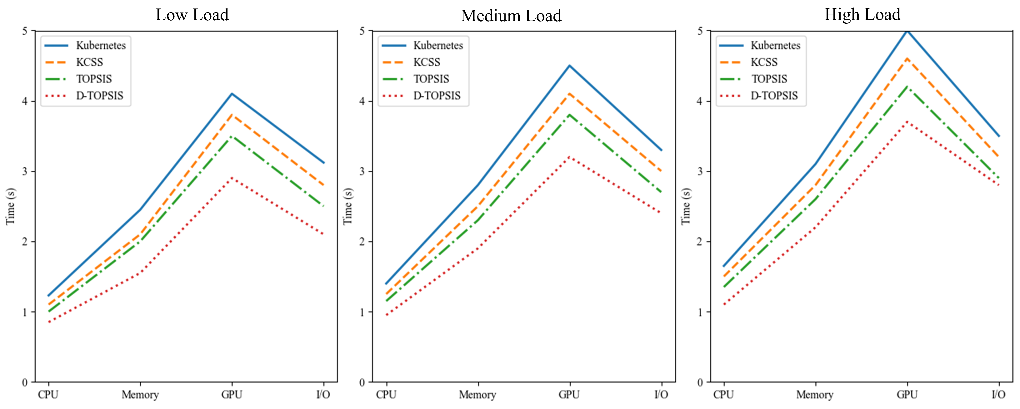
The task response times of the different algorithms under varying load conditions are shown in Figure 2. The horizontal axis represents the resource requirements for various task types, while the vertical axis displays the corresponding response times. As illustrated in the figure, the D-TOPSIS algorithm consistently outperformed the other algorithms in terms of response time, particularly for CPU-bound tasks, where it demonstrated superior efficiency in allocating CPU resources. As the memory requirements increased, D-TOPSIS maintained the lowest response time, further showcasing its ability to handle memory-intensive tasks effectively. For GPU-intensive tasks, D-TOPSIS achieved the shortest response time, reflecting its adeptness in dynamically adjusting GPU resource weights. Additionally, the algorithm also exhibited the lowest response time for I/O-bound tasks. These results collectively demonstrate that D-TOPSIS achieved consistently lower response times across all resource dimensions, validating the efficacy of its dynamic resource weight adjustment strategy in optimizing task scheduling.

4.3.2. System Throughput Testing and Analysis

Throughput performance is shown in

Table 4. Throughput comparison (unit: tasks per second).

Load Condition	Type of Task	Kubernetes	KCSS	TOPSIS	D-TOPSIS
Low load	CPU	90	95	100	115
Low load	Memory	45	52	55	70
Low load	GPU	50	55	60	60
Low load	I/O	38	42	50	55
Medium load	CPU	85	90	100	110
Medium load	Memory	42	50	59	63
Medium load	GPU	70	75	85	95
Medium load	I/O	35	40	50	52
High load	CPU	80	85	90	105
High load	Memory	40	48	50	60
High load	GPU	60	65	80	100
High load	I/O	33	38	45	48

, further supporting the effectiveness of the D-TOPSIS algorithm in high-load scenarios. The results indicate that D-TOPSIS consistently outperformed the other scheduling methods across all load conditions, including high load. Notably, under high-load conditions involving GPU-intensive tasks, D-TOPSIS achieved a 53.8% improvement in throughput over the KCSS algorithm, with throughput increasing from 65% to 100%. This demonstrates that our dynamic scheduling approach can effectively mitigate resource bottlenecks, even when the system faces heavy demand, ensuring optimal utilization of resources. Additionally, in memory-intensive and I/O-bound tasks, D-TOPSIS maintained high throughput, further emphasizing its capability to handle high-load scenarios efficiently.

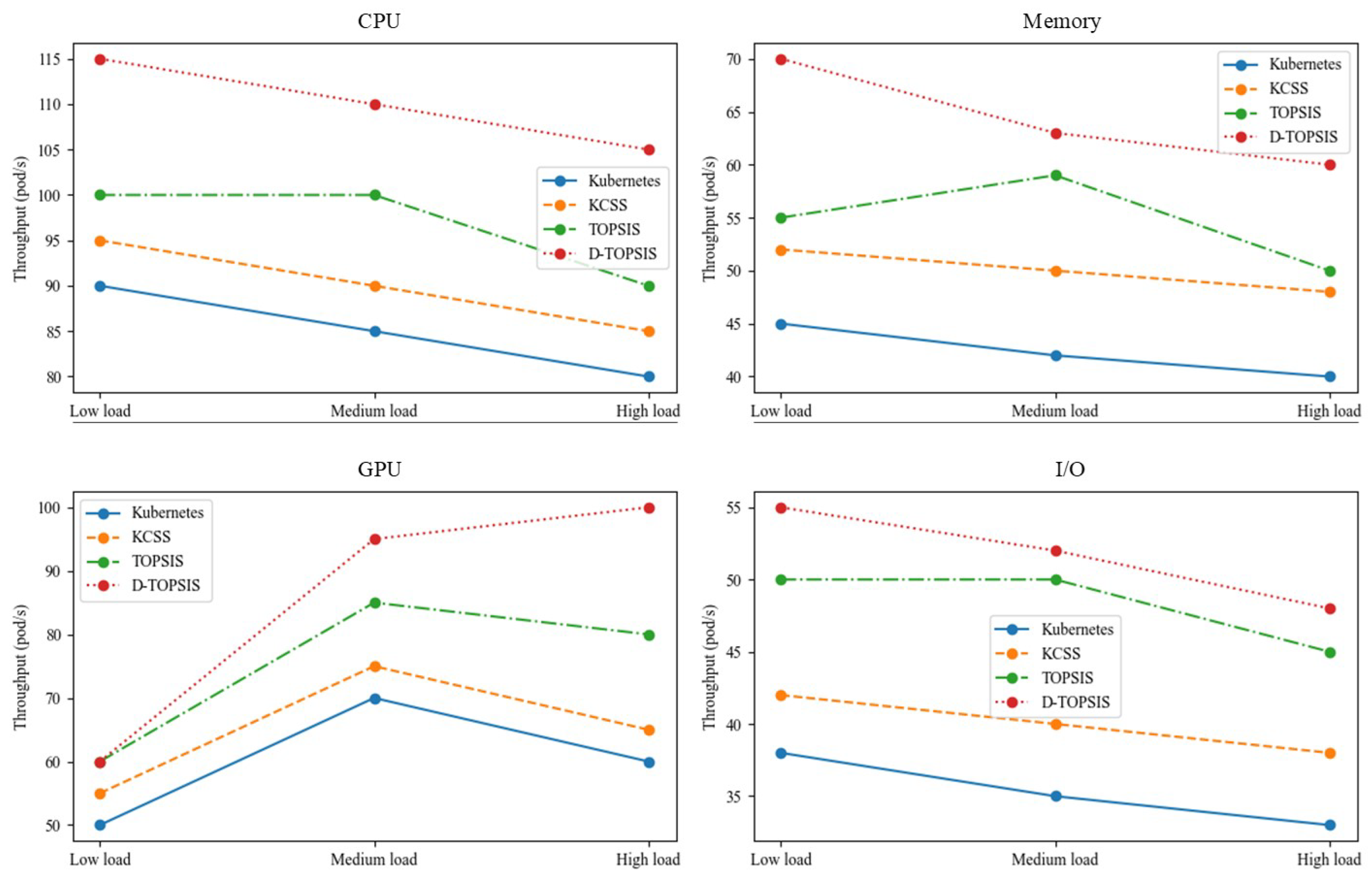
The throughput performance of each algorithm under varying load conditions was analyzed in detail. As illustrated in Figure 3, the D-TOPSIS algorithm consistently outperformed all other algorithms in terms of throughput across the different load scenarios and task types. This highlights its superior capability in dynamic resource scheduling. Under low-load conditions, the D-TOPSIS algorithm effectively optimized resource utilization, leading to a significant increase in throughput.

As the system load increased, the D-TOPSIS algorithm maintained a high throughput by dynamically adjusting resource allocation to meet the changing demands. In contrast, the other algorithms struggled to sustain optimal throughput, particularly under medium- and high-load conditions, due to less efficient resource allocation strategies. These findings emphasize the D-TOPSIS algorithm’s robustness and adaptability, demonstrating its effectiveness in optimizing throughput across a wide range of workloads and environments.

The D-TOPSIS algorithm showed impressive results not only under low-load conditions but also in high-load scenarios. While the improvements in task response time and throughput were somewhat smaller under heavy loads due to increased resource contention, the D-TOPSIS algorithm still outperformed the other advanced scheduling methods in terms of both task scheduling efficiency and resource utilization. These results highlight the scalability and robustness of our approach, making it well-suited for dynamic cloud environments that experience fluctuating load conditions.

The proposed D-TOPSIS algorithm consistently outperformed the Kubernetes default scheduler, the KCSS algorithm, and the traditional TOPSIS algorithm in terms of throughput across all test scenarios. Under low-load conditions with memory-intensive tasks, D-TOPSIS achieved a throughput increase of 45% to 70% (a 55.6% improvement) compared to Kubernetes. Similarly, in GPU-intensive tasks under high-load conditions, D-TOPSIS demonstrated a 53.8% improvement in throughput over the KCSS algorithm, with throughput rising from 65% to 100%.

These results emphasize the algorithm’s robustness and scalability, demonstrating that as the system load increases—whether in terms of task volume or resource demand—D-TOPSIS effectively handles larger task volumes and greater resource requirements. Even in resource-intensive scenarios, the dynamic scheduling approach mitigates bottlenecks, ensuring efficient performance and consistent throughput. This confirms that the D-TOPSIS algorithm is capable of scaling with increased numbers of tasks and resources, significantly enhancing the system’s task processing capacity without substantial performance degradation.

4.3.3. Resource Utilization Testing and Analysis

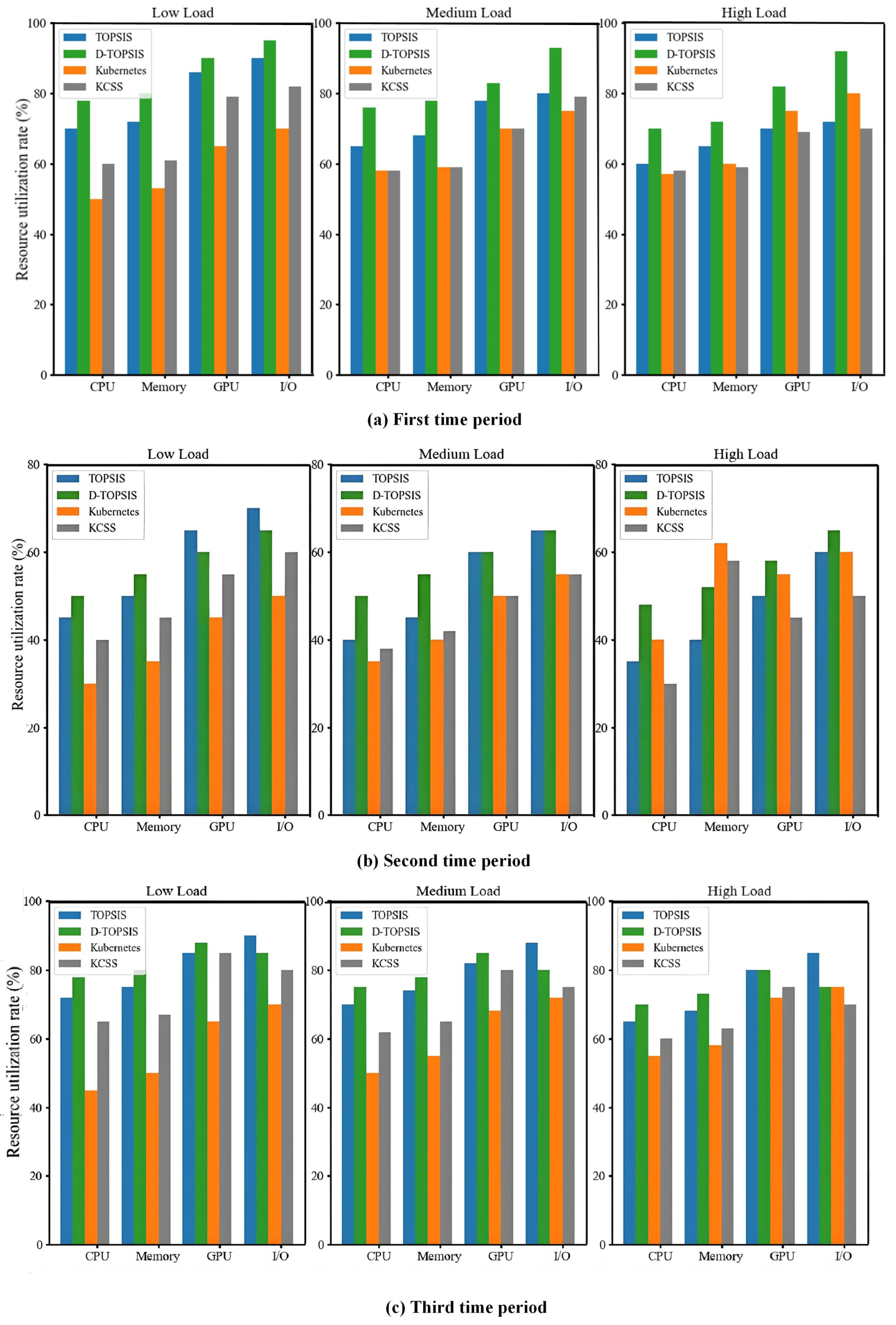
The resource utilization of various scheduling algorithms was assessed over three 30-min intervals, with data collected at the start (0 min), midpoint (15 min), and end (30 min) of each interval. As shown as in the

Table 5. Resource utilization under different scheduling algorithms.

Load	Type	Kubernetes	KCSS	TOPSIS	D-TOPSIS
Low	CPU	76%/72%/50%	80%/75%/55%	90%/85%/60%	95%/90%/65%
Low	Memory	68%/78%/45%	72%/80%/50%	85%/88%/65%	90%/85%/70%
Low	GPU	50%/45%/30%	55%/50%/35%	70%/65%/45%	75%/70%/50%
Low	I/O	60%/65%/40%	62%/67%/45%	80%/85%/55%	85%/80%/60%
Medium	CPU	74%/70%/50%	78%/74%/55%	88%/82%/60%	92%/88%/65%
Medium	Memory	65%/75%/40%	70%/78%/45%	80%/85%/60%	85%/80%/65%
Medium	GPU	55%/50%/35%	58%/55%/40%	72%/68%/50%	78%/72%/55%
Medium	I/O	58%/62%/38%	60%/65%/42%	75%/80%/50%	80%/75%/55%
High	CPU	70%/65%/48%	72%/68%/52%	85%/80%/58%	90%/85%/65%
High	Memory	60%/70%/35%	65%/73%/40%	75%/80%/50%	80%/75%/60%
High	GPU	60%/55%/40%	62%/58%/45%	76%/72%/55%	80%/75%/60%
High	I/O	55%/60%/30%	58%/63%/35%	70%/75%/45%	75%/70%/50%

, the resource utilization remained relatively low under low-load conditions, increasing with the load. The D-TOPSIS algorithm consistently ensured high resource utilization across CPU, memory, and I/O, whereas both Kubernetes and KCSS exhibited more conservative resource allocation, especially in memory and I/O. During high-load conditions, the resource utilization increased across all algorithms, often reaching or approaching peak values. The benefits of D-TOPSIS were most evident in high-load scenarios, where it optimally utilized CPU, memory, and I/O resources. These findings highlight that D-TOPSIS efficiently allocates resources in high-demand environments, alleviating resource contention and preventing inefficiencies stemming from underutilization.

The resource utilization performance of each scheduling algorithm was evaluated across low, medium, and high load scenarios, as shown in Figure 4. In the low-load case, D-TOPSIS achieved approximately 95% CPU utilization, significantly outperforming Kubernetes and KCSS. For memory resources, it achieved 90% utilization, while the other algorithms only achieved 68% and 72%, respectively. This highlights D-TOPSIS’s ability to optimize resource usage in low-load conditions, improving overall system performance and efficiency. In the medium-load scenario, D-TOPSIS maintained a high utilization, with memory usage reaching 85%, about 20 percentage points higher than Kubernetes, demonstrating its ability to balance resource allocation effectively, avoiding both underutilization and shortages.

In the high-load case, D-TOPSIS achieved 80% GPU and 75% I/O utilization, compared to only 60% GPU and 55% I/O utilization with Kubernetes. These results emphasize D-TOPSIS’s superior load-balancing capabilities, especially under high-load conditions, where it optimizes resource allocation and maintains system stability. Overall, D-TOPSIS consistently outperformed the other algorithms across varying load conditions, validating its potential for enhancing resource management and performance in dynamic and complex environments.

5. Conclusions

In this paper, we propose a dynamic, multi-dimensional heterogeneous resource scheduling method for Kubernetes that combines a dynamic resource weight adjustment strategy with an enhanced TOPSIS algorithm. This approach overcomes the limitations of traditional scheduling techniques by optimizing task scheduling in real time, reducing resource wastage and delays caused by uneven resource allocation. Experimental results showed that our method outperformed the default Kubernetes scheduler and the KCSS algorithm under low-load conditions, achieving a 31% to 36% reduction in task response time, a 20% to 50% increase in throughput, and a 20% improvement in resource utilization.

Despite these gains, challenges persist in more complex environments with diverse resources, such as specialized hardware accelerators like FPGAs or TPUs. As the cluster size increases, computational overhead may impact scalability and response time. Furthermore, although the load balancing has been improved, certain task types still experience suboptimal distribution, leading to resource underutilization. In future work, we will refine the load balancing strategy to enable more dynamic adjustments based on system load fluctuations. We also plan to improve the scalability and adaptability, allowing the method to handle a wider range of resources and more complex interactions. These efforts will optimize resource utilization and scheduling performance, ensuring efficient operation in large-scale, diverse environments.