A Novel SHAP-GAN Network for Interpretable Ovarian Cancer Diagnosis

Abstract

Ovarian cancer stands out as one of the most formidable adversaries in women’s health, largely due to its typically subtle and nonspecific early symptoms, which pose significant challenges to early detection and diagnosis. Although existing diagnostic methods, such as biomarker testing and imaging, can help with early diagnosis to some extent, these methods still have limitations in sensitivity and accuracy, often leading to misdiagnosis or missed diagnosis. Ovarian cancer’s high heterogeneity and complexity increase diagnostic challenges, especially in disease progression prediction and patient classification. Machine learning (ML) has outperformed traditional methods in cancer detection by processing large datasets to identify patterns missed by conventional techniques. However, existing AI models still struggle with accuracy in handling imbalanced and high-dimensional data, and their “black-box” nature limits clinical interpretability. To address these issues, this study proposes SHAP-GAN, an innovative diagnostic model for ovarian cancer that integrates Shapley Additive exPlanations (SHAP) with Generative Adversarial Networks (GANs). The SHAP module quantifies each biomarker’s contribution to the diagnosis, while the GAN component optimizes medical data generation. This approach tackles three key challenges in medical diagnosis: data scarcity, model interpretability, and diagnostic accuracy. Results show that SHAP-GAN outperforms traditional methods in sensitivity, accuracy, and interpretability, particularly with high-dimensional and imbalanced ovarian cancer datasets. The top three influential features identified are PRR11, CIAO1, and SMPD3, which exhibit wide SHAP value distributions, highlighting their significant impact on model predictions. The SHAP-GAN network has demonstrated an impressive accuracy rate of 99.34% on the ovarian cancer dataset, significantly outperforming baseline algorithms, including Support Vector Machines (SVM), Logistic Regression (LR), and XGBoost. Specifically, SVM achieved an accuracy of 72.78%, LR achieved 86.09%, and XGBoost achieved 96.69%. These results highlight the superior performance of SHAP-GAN in handling high-dimensional and imbalanced datasets. Furthermore, SHAP-GAN significantly alleviates the challenges associated with intricate genetic data analysis, empowering medical professionals to tailor personalized treatment strategies for individual patients.

1. Introduction

Despite the rapid development of medical technologies, many treatment methods for ovarian cancer have also increased over the years [1]. Nevertheless, the conventional approach continues to be chemotherapy, a practice that has endured over the last twenty years [2]. Most patients gradually develop resistance to this treatment, leading to deteriorating treatment outcomes in the later stages [3]. Therefore, early diagnosis and personalized treatment plans are particularly important. Ovarian cancer is frequently diagnosed in advanced stages due to the lack of clear early clinical symptoms, thereby contributing to its status as the fifth deadliest cancer among women [4]. Existing early diagnostic methods are divided into biomarker detection and imaging diagnosis. Although these technologies can aid in ovarian cancer diagnosis to a certain degree, their accuracy remains limited, frequently resulting in incorrect assessments or misdiagnoses [5]. For asymptomatic women, routine ovarian cancer screening is often not recommended, as there is no strong scientific evidence supporting the idea that it reduces ovarian cancer mortality [6].

In recent years, scientists have discovered that ovarian cancer is a highly heterogeneous malignant tumor, and its occurrence and development are closely related to various genetic factors [7]. Studies show that the development of ovarian cancer is not only influenced by environmental factors and lifestyle but also by genetic mutations, abnormal regulation of gene expression, and changes in the tumor microenvironment, all of which play key roles in ovarian cancer progression [8]. Specific genetic variations and changes in gene expression patterns are often critical for early diagnosis and disease prognosis prediction in ovarian cancer [9]. Therefore, identifying genetic biomarkers associated with ovarian cancer can help us better understand its molecular mechanisms and provide new insights for early diagnosis and personalized treatment [10]. As a result, biomarkers significantly enhance the sensitivity and accuracy of disease detection by providing disease-specific molecular signatures, offering critical support for early diagnosis and personalized treatment [11]. Among these biomarkers, CA125 has long been regarded as the most promising biomarker for detecting ovarian cancer. However, other diseases can also cause elevated CA125 levels, indicating its lack of sensitivity [12]. HE4, another ovarian cancer biomarker, is highly expressed in ovarian cancer patients [13], but other malignancies can also elevate HE4 levels [14]. Due to the low sensitivity of these biomarkers, researchers have turned to alternative diagnostic models, such as the Risk of Ovarian Malignancy Algorithm (ROMA). This model incorporates markers like HE4 and CA125, along with menopausal status, to assess a woman’s likelihood of having ovarian cancer [15]. Experiments also showed that this model demonstrates higher accuracy and sensitivity compared to using CA125 and HE4 alone [16].

With the rapid development of artificial intelligence technologies, massive clinical data accumulated worldwide is being gradually utilized. ML and DL, in the field of AI, have shown better performance in cancer diagnosis and prediction compared to traditional methods [17]. Lu et al. studied the application of AI methods in ovarian tumor malignancy prediction, using Logistic Regression and multi-layer perceptron (MLP) algorithms. Their results showed that this algorithm significantly improved the prediction accuracy, achieving an AUC value of 95.4% [18]. Lee et al. used Generative Adversarial Networks (GANs) for data augmentation on an asthma dataset, achieving a prediction accuracy of 94.3% [19]. One can observe that, owing to its remarkable processing speed, an increasing number of AI technologies are being utilized as medical assistive tools in cancer diagnosis [20]. However, AI faces challenges such as declining prediction accuracy when dealing with imbalanced and high-dimensional datasets. Additionally, since traditional ML models are considered “black-box” processes, interpreting these models is highly challenging. With the emergence of generative network models, the issue of data imbalance has been addressed [21], but typical GANs often lack attention to input sample features, which can result in generated samples that may not have real biological significance. This paper proposes an innovative data augmentation module that effectively focuses on important sample features and designs a comprehensive ovarian cancer diagnostic model to address these issues.

The structure of this paper is outlined as follows: Section 2 offers an overview of the dataset and delves into the fundamental principles underpinning SHAP and GAN. The methodology introduced in this study is elaborated in Section 3. Section 4 examines the efficacy of the proposed approach, juxtaposes it against alternative models, and elaborates on the results comprehensively. Finally, Section 5 wraps up with a concise summary of the discoveries.

2. Materials and Methods

In ovarian cancer gene research, gene expression profiling and gene mutation detection have proven to be critical tools for diagnosis and prognosis assessment. For example, high-throughput genomics techniques for analyzing ovarian cancer gene expression can reveal the overexpression or suppression of specific genes, providing strong evidence for early cancer screening. Moreover, gene mutations and epigenetic abnormalities are closely associated with ovarian cancer development, and these genetic changes could serve as potential targets for targeted therapy in cancer diagnosis and treatment.

This research makes use of gene expression data from six ovarian cancer microarray datasets, which are publicly available on the Kaggle platform. These datasets include GSE6008, GSE9891, GSE18520, GSE38666, GSE66957, and GSE69428 [22,23]. The dataset comprises 502 ovarian cancer samples representing five different ovarian cancer types, providing a rich basis for this study. By performing feature selection and analysis on these datasets, the research aims to explore key genes and features associated with ovarian cancer, ultimately revealing potential biomarkers for the disease. These genes and features not only help identify early signs of cancer but also offer more targeted support for personalized treatment. Figure 1 depicts the class distribution of the original dataset, highlighting the significant imbalance between classes within the ovarian cancer data. Specifically, the number of samples in class 2 far exceeds that of other types, which may affect the model’s training performance and prediction accuracy. Figure 2 reveals the correlations between different features through Pearson correlation analysis and identifies which features are more strongly correlated with the target variable (ovarian cancer type). The top ten features in Figure 2 were selected using the XGBoost algorithm. Through Figure 2, we can detect multicollinearity among these features, thereby providing intuitive guidance for subsequent model construction. This is because high correlations between certain features may lead to model overfitting or reduce model interpretability in machine learning. By analyzing these correlations, the most representative and independent features can be selected. 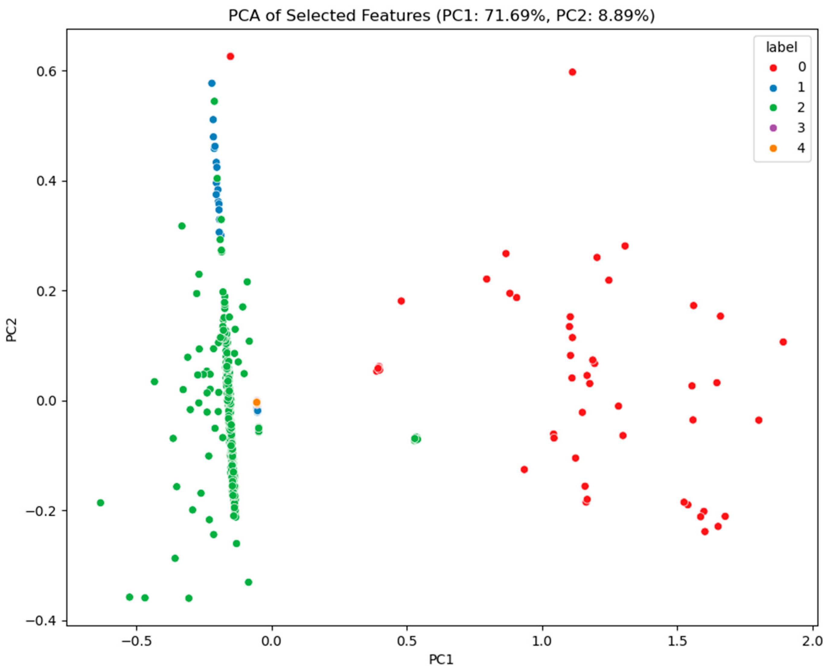Figure 3, through dimensionality reduction visualization, illustrates the separation between different ovarian cancer types, demonstrating the biological differences among cancer subtypes. The distinct separation between categories in the feature space establishes a solid foundation for future classification models. To further enhance model performance, the XGBoost algorithm was employed to rank feature importance and select the top 10 most predictive features [24,25]. These features have potential clinical significance for ovarian cancer diagnosis and treatment.

Table 1. The traits of the ovarian cancer dataset.

No	Feature Name	Remarks
1	CHTOP	Helps control gene activity and may influence tumor growth by regulating gene expression.
2	ABCA5	Involved in lipid transport, affecting cell membrane structure and metabolism, which is often altered in cancer cells.
3	OSBP	Helps control lipid balance in cells, and its disruption can affect cancer cell growth and spread.
4	SMBP3	Part of a pathway that regulates cell growth; can either stop or promote cancer, depending on the context.
5	JTB	Affects cell adhesion, and its malfunction may help cancer cells spread to other parts of the body.
6	BEST1	A protein that controls ion transport; its abnormal function can lead to cancer by disrupting cell growth and death.
7	CIAO1	Involved in iron metabolism, which is often disrupted in cancer cells to support their energy needs.
8	ABHD11	Regulates lipids in cells, and its function can influence cancer cell growth.
9	PRR11	May help control the cell cycle; its abnormal levels could support cancer cell survival and growth.
10	ACSM1	Involved in fatty acid metabolism, which is crucial for cancer cells to thrive and grow.

lists these key features and briefly introduces their biological functions in the human body. Through in-depth analysis of the ovarian cancer gene datasets, it is possible to provide more accurate and effective tools for early diagnosis, treatment decision-making, and prognosis evaluation of ovarian cancer.

As this study focuses on the SHAP-GAN network for ovarian cancer diagnosis, this section offers a concise overview of SHAP and GAN components.

2.1. A Brief Description of SHAP

The training process of ML models is often considered opaque. Data are input into the model, and the model adjusts its parameters by learning from these data, ultimately being able to make predictions on new data. However, during this process, it is often difficult to understand how each input feature influences the model’s final prediction. SHAP values provide a method to uncover this “black box”. It draws on the concept of Shapley values from game theory to explain and quantify the specific contribution of each feature to the model’s prediction. By calculating SHAP values, we can understand which input features played a key role when the model made a particular prediction and how they collectively influenced the prediction result.

Originally, Shapley values were introduced by Lloyd Shapley as a mathematical tool in cooperative game theory to fairly distribute the gains from cooperation [26]. In 2010, Erik Štrumbelj et al. first applied this theory to ML to explain the prediction mechanisms of models [27]. Then, in 2017, Scott Lundberg et al. further developed the concept of SHAP (SHapley Additive explanations), positioning it as an important tool for explaining ML models. They built a theoretical framework connecting SHAP with other interpretability techniques like LIME and DeepLIFT, opening up new pathways for interpretability research in ML models [28].

Shapley aims to resolve conflicts arising from the distribution of benefits among participants in a cooperative process. The fundamental idea is to evaluate the incremental impact of each team member on the collective value of the team and subsequently distribute the rewards equitably according to these contributions. The formula for calculating the Shapley value is as follows. Here, ${\varphi }_i\left(v\right)$ represents the Shapley value of the i-th participant under the value function v. N represents the total number of participants in the team, S is a subset of participants excluding iii, and |S| represents the number of participants in subset S. |N| represents the total number of participants in the team. $v(S\cup \{i\left\}\right)$ represents the value contributed by participant i to the team, and $v\left(S\right)$ represents the value of the team S after excluding participant i.

$${\varphi }_i(v)=\sum _{S\subseteq N\setminus \left\{i\right\}}{\displaystyle \frac{\left|S\right|!\left(\right|N|-|S|-1)!}{\left|N\right|!}}(v(S\cup \{i\})-v(S))$$

(1)

The Shapley value is characterized by four key properties: efficiency, symmetry, dummy player, and additivity. Efficiency indicates that the sum of all team members’ Shapley values equals the total expenditure. Symmetry means that if two players contribute equally to the team’s value, their corresponding Shapley values are also equal. A dummy player refers to a player whose contribution to the team is zero, in which case their Shapley value is zero. Additivity means that if there are two value functions v and u, and two arbitrary constants a and b, then the Shapley value for a member is the linear combination of their Shapley values under v and u. The formulas for these four properties are as follows.

$$\sum _{i=1}^n{\varphi }_i(v)=v(N)-v(\varnothing )$$

(2)

$$IF \forall S\subseteq \{1,\dots ,p\}\setminus \{j,k\}, val(S\cup \{j\left\}\right)=val(S\cup \{k\left\}\right) than {\varphi }_j={\varphi }_k$$

(3)

$$IF \forall S\subseteq \{1,\dots ,p\}, val(S\cup \{j\left\}\right)=val\left(S\right) than {\varphi }_j=0$$

(4)

$${\varphi }_i(av+bu)=a{\varphi }_i\left(v\right)+b{\varphi }_i\left(u\right)$$

(5)

SHAP is an efficient algorithm based on Shapley values, and it provides explanations for predictions made by black-box models in ML. By calculating the contribution of each input feature, SHAP helps us analyze and understand why the model makes a particular prediction.

2.2. A Brief Description of GANs

GAN is a revolutionary generative model proposed by Ian Goodfellow and others in 2014, which significantly accelerated advancements in ML, particularly in the field of generative modeling [29]. The core idea of a GAN is to create an adversarial training environment consisting of two main components: the generator (G) and the discriminator (D). These two neural networks compete with each other during training, optimizing, and adjusting through an iterative process that gradually approaches a balanced state—known as a Nash equilibrium. Specifically, the goal of a GAN is to design a bidirectional adversarial training mechanism by minimizing the generator’s loss function and maximizing the discriminator’s loss function, allowing the generator to learn to produce increasingly realistic samples, while the discriminator continuously improves its ability to distinguish between real and fake samples. The loss function can be expressed by the following formula:

$$\underset{G}{min}\underset{D}{max}V(D,G)=E_{x\sim p_{data}(x)}[logD(x)]+E_{z\sim p_z(z)}[log(1-D(G(z)))]$$

(6)

The original Generative Adversarial Network (GAN) had relatively basic functionality, only being able to generate simple samples based on the given data. However, over time, researchers have made several improvements to GAN, expanding its applications in different fields. In the area of image processing, Koo et al. adopted the Deep Convolutional GAN (DCGAN), enabling the automatic colorization of black-and-white images [30]. At the same time, the Conditional GAN (cGAN) was introduced, which integrates conditional information to ensure that the generated samples align with the training data distribution while also meeting specific conditions [31]. In 2016, Odena et al. introduced the Auxiliary Classifier GAN (ACGAN), a novel extension of the cGAN architecture that incorporates an auxiliary classifier. By integrating this classifier, the ACGAN enabled both the generator and discriminator to make use of classification information, leading to an enhancement in the diversity and quality of the generated samples [32]. The architecture of the ACGAN is illustrated in Figure 4. In addition to the traditional binary cross-entropy loss used for discriminating between real and fake samples, a supplementary classification loss function was incorporated to optimize classification tasks. This adjustment empowered the discriminator to acquire more comprehensive feature representations, thereby enhancing its learning capabilities.

For GANs, the optimization of the generator’s parameters occurs through the conventional adversarial training process, wherein a dynamic interplay unfolds between the generator and discriminator. The primary objective of the generator is to craft authentic-looking samples, counterbalanced by the discriminator’s task of distinguishing between real and synthetic data samples. Although this process is effective, it does not directly consider the specific contribution of each feature to the generated output, nor does it provide fine-grained adjustments to the generator’s parameters. The generator optimization focuses on enhancing the collective quality of the generated samples, rather than scrutinizing and fine-tuning the influence of specific features. The generator relies solely on the feedback from the discriminator to learn the feature distributions, but it does not know which input features are more crucial for improving the quality of the generated samples. This becomes particularly challenging in high-dimensional or complex datasets, where the generator may struggle to capture the subtle relationships between features.

3. The Proposed Method

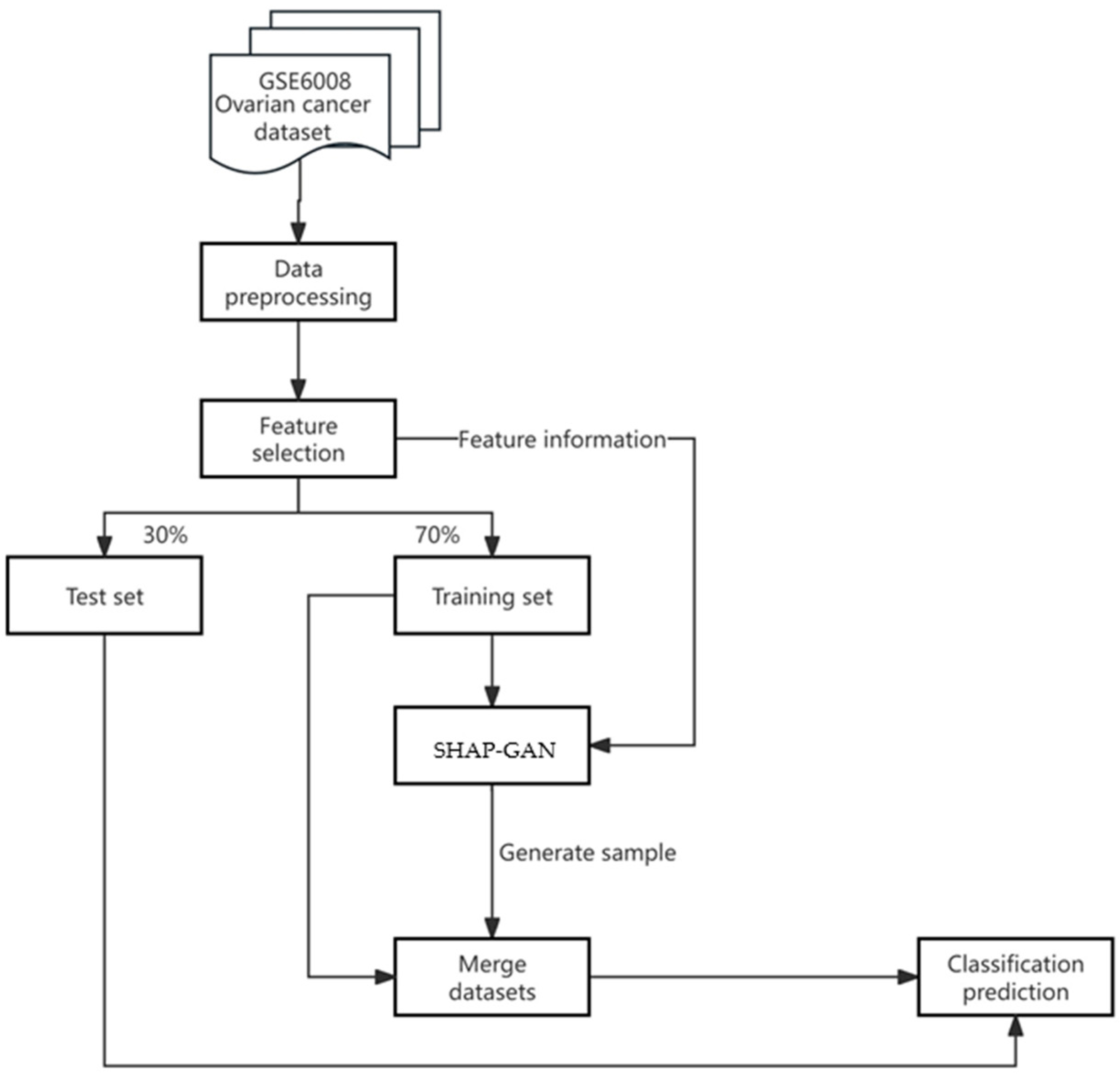
This research presents a groundbreaking SHAP-GAN network tailored for the precise diagnosis of ovarian cancer. Integrating the interpretability of SHAP with the data generation capabilities of a GAN, the innovative approach is geared towards enhancing diagnostic precision. The methodology’s flowchart, depicted in Figure 5, elaborates on every stage of the process, starting from data preprocessing and culminating in model output.

The dataset used in this study for ovarian cancer encompasses five different types of ovarian cancer, along with information on more than 10,000 related genes. To improve data accuracy and eliminate batch effects, the PyComBat 0.4.4. tool is applied to process these datasets and normalize features in the data preprocessing. Although the dataset provides rich information for cancer research, handling such a large dataset presents a significant challenge for physicians in practical applications. Relying on these gene data for preventive diagnosis would burden doctors, making it difficult to quickly and accurately extract key information for diagnosis. To overcome this challenge, XGBoost 2.1.4. was used to select features. Additionally, there is a severe data imbalance issue in the dataset, with certain types of ovarian cancer having far fewer samples than others. Data imbalance can lead to poor learning performance for the minority classes, affecting the accuracy of recognizing these rare types. Given the complexity and lethality of ovarian cancer, it is crucial to ensure that the model can effectively distinguish all types of cancer to avoid misdiagnosis or missed diagnosis. The proposed algorithm includes the SHAP-GAN data augmentation technique followed by using the XGBoost model for classification. It should be noted that the SHAP-GAN was only applied to the training set to augment data.

The SHAP-GAN network integrates SHAP values into the generator of a GAN network as shown in Figure 6.

Since SHAP values can evaluate the importance of each feature for predictive classification, they can guide the generator on how to better capture the key features of real data, thereby enhancing the diversity and realism of the generated samples. The main structure of SHAP-GAN is illustrated in Figure 6. The generator adjusts its parameters based on the SHAP values, modifying the activation strength of each feature when generating samples. For important features, the generator increases their influence by amplifying their contribution to the generation process, ultimately improving the performance of these key features in the final generated samples. Designing the loss function for a SHAP-GAN involves combining the traditional GAN loss with SHAP values to ensure that the generated samples are not only realistic but also have meaningful attributions based on the SHAP values. The traditional GAN loss function can be expressed as Equation (6). SHAP values provide feature attributions for a model’s predictions, indicating the impact of each feature on the model’s output. In the context of a SHAP-GAN, SHAP values can be used to guide the generation process toward producing samples with meaningful attributions. Let $\mathrm{\varnothing }\left(x\right)$ represent the SHAP values for the features of sample $x$. The SHAP loss component can be defined as the discrepancy between the SHAP values of the generated samples $G\left(z\right)$ and real data x. The SHAP loss could be:

$$L_{SHAP}=Loss\_Function(\mathrm{\varnothing }\left(x\right),\mathrm{\varnothing }(G\left(z\right)\left)\right)$$

(7)

where Loss_Function is a distance metric to measure the difference between the SHAP values. The overall loss function for the SHAP-GAN can be shown as follows.

$$L_{SHAP-GAN}={-E}_z\left[\log D\left(G\left(z\right)\right)\right]+L_{SHAP}$$

(8)

By combining the GAN loss with the SHAP loss component, the SHAP-GAN is trained to generate samples that not only appear realistic but also have meaningful feature attributions based on the SHAP values. During training, the SHAP-GAN is optimized to minimize the combined loss function, which encourages the generator to not only produce realistic samples but also samples that align with meaningful feature attributions provided by the SHAP values.

4. Results and Discussion

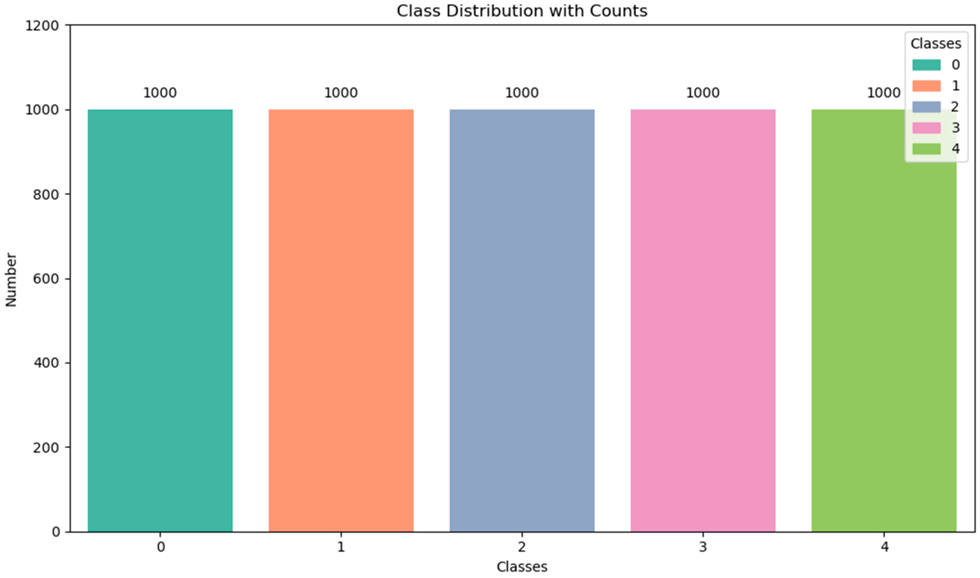
The study utilizes an NVIDIA 4060 graphics card and Python 3.9 for programming, in conjunction with TensorFlow-GPU version 2.7. In the SHAP-GAN architecture, the Adam optimizer is utilized to fine-tune the weight parameters, with a learning rate configured at 0.0002. Specifically, the SHAP-GAN network generates 1000 samples for every subtype of ovarian cancer, and the exact distribution of samples is detailed in Figure 7. After augmenting the original dataset, the sample distribution becomes more evenly balanced.

Figure 8 illustrates the impact of different feature dimensions on the model’s classification accuracy. From the figure, it is evident that as the feature dimension increases to 10, the model’s accuracy stabilizes at 99.34% from XGBoost. This suggests that after reaching a certain dimension, adding more features contributes negligibly to the model’s performance. From a practical perspective, it is ideal for physicians to maintain the same accuracy while reducing the number of required features to streamline the diagnostic process. To delve further into the implications of these 10 features on the model, the SHAP-GAN network was employed to evaluate their impact, enabling an accurate measurement of the significance of each feature on the model’s predictions.

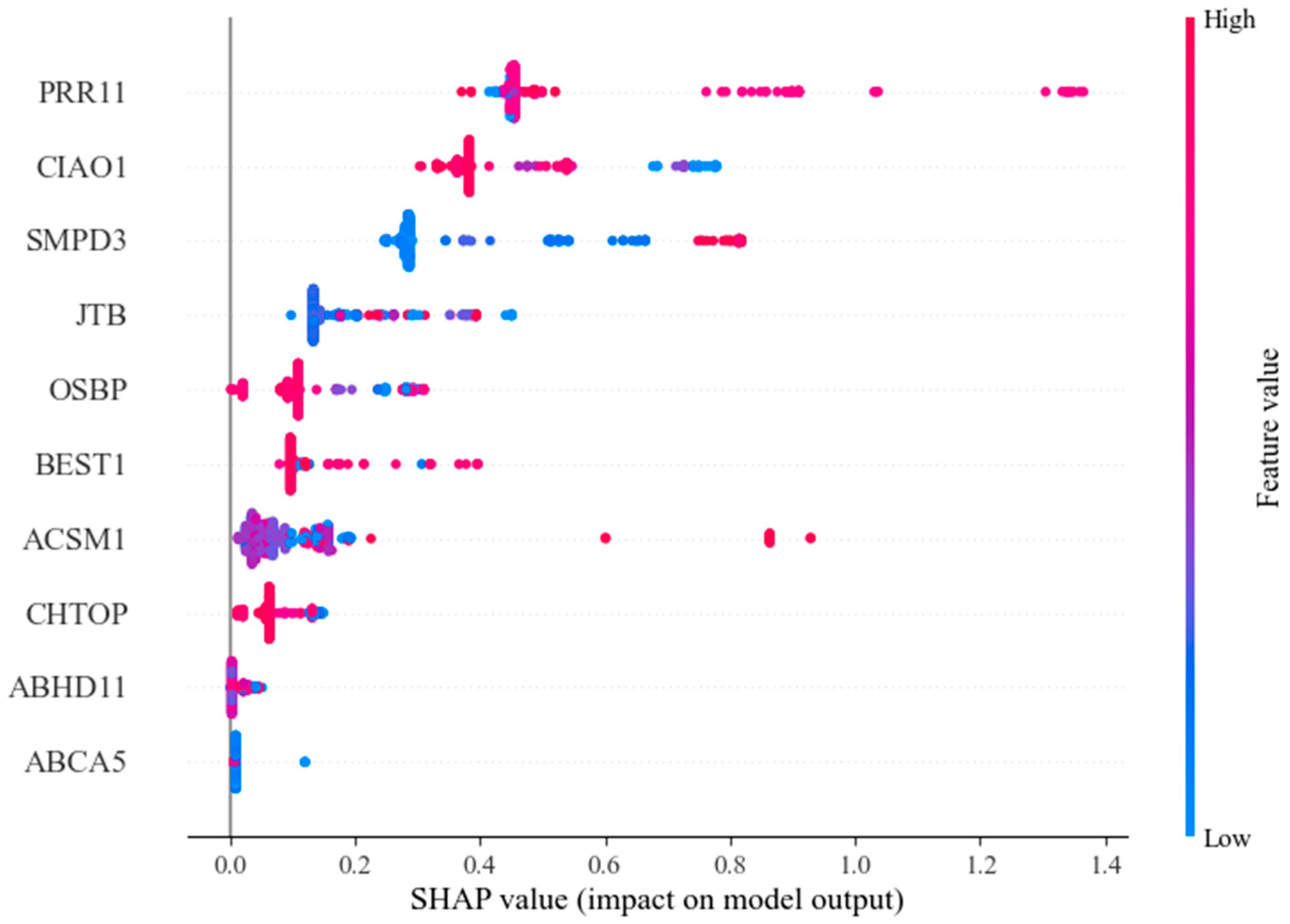
Figure 9 showcases the SHAP values associated with each feature, where the horizontal axis denotes the SHAP value. This axis elucidates the extent to which each feature influences the ultimate prediction, providing crucial insights into the significance and function of each feature within the model’s decision-making framework. The vertical axis lists the feature names. The color gradient from blue to red indicates the change in feature value from low to high, and the distribution of points reveals the relationship between feature values and SHAP values. This helps to understand whether each feature has a positive or negative impact on the model’s prediction and sheds light on the decision-making process of the model. From the figure, it is evident that after feature selection, all features exert a positive influence on the model. The top three features with the greatest influence are PRR11, CIAO1, and SMPD3. The SHAP value distribution of these three factors is quite broad, indicating their significant impact on the model’s output. PRR11, a proline-rich protein, plays a crucial role in regulating the cell cycle, with its dysregulated expression potentially fueling the growth and survival of cancerous cells. On the other hand, CIAO1 is intricately linked to endocytosis and the transport of proteins within the cell, exerting a significant influence on the integrity and functionality of the cell membrane. In cancer cells, CIAO1 may promote tumor cell proliferation and metastasis, and its abnormal expression may alter the intracellular protein localization, thereby impacting cell proliferation, migration, and anti-apoptotic functions. SMPD3 is responsible for encoding a sphingomyelin phosphodiesterase, crucial for the degradation of sphingolipids that play a vital role in preserving the integrity and signaling of cell membranes. Any irregularities in these genes may disrupt essential cellular functions like growth, metabolism, and migration, all of which are significant contributors to cancer progression.

To enhance the reliability of the proposed model, a thorough validation process employing 5-fold cross-validation was conducted. Initially, the dataset was randomly segmented into five subsets, with each subset serving as the test set once, while the remaining four subsets were allocated for training purposes. Subsequently, the model underwent training on the training data in each cycle, followed by an evaluation of the corresponding validation set. This iterative procedure was reiterated five times to ensure that each subset underwent individual evaluation. The outcomes of this experimentation have been succinctly presented in

Table 2. The cross-validation outcomes of the model for the ovarian cancer dataset.

Experiment	Accuracy (%)	Precision (%)	Recall (%)	F1 Score (%)
#1-Fold	98.98	98.30	98.98	98.57
#2-Fold	98.98	98.30	98.98	98.57
#3-Fold	100.00	100.00	100.00	100.00
#4-Fold	95.92	96.10	95.92	95.76
#5-Fold	94.55	94.46	94.55	94.44

. The optimal results derived from the cross-validation affirm that the model exhibited impeccable performance across all assessment metrics, encompassing accuracy, precision, recall, and F1 score. Notably, the marginal performance discrepancies observed between the folds underscore the model’s consistent efficacy across diverse data segments. This uniformity underscores the model’s exceptional generalization capability and resilience. Irrespective of the subset utilized for testing, the model consistently and accurately predicted occurrences of ovarian cancer, underscoring its robust classification prowess. The negligible performance variations observed across folds further validate the model’s reliability, suggesting that it can maintain stable and efficacious outcomes even with varying data splits.

In order to offer a more thorough assessment of the effectiveness of the proposed algorithm, a comparative analysis was conducted against various well-established classification techniques, in addition to commonly employed methodologies from the Kaggle platform [22]. To ensure fairness in the experiments, the same data subsets were used for all comparison experiments, and each model was trained and tested in a consistent experimental environment. The comparison results are detailed in

Table 3. The performance comparison of various methods.

Method	Classification Accuracy (%)
SVM	82.78
LR	86.09
Kaggle [22]	94.06
XGBoost	96.69
The integrated algorithm [23]	99.01
The proposed SHAP-GAN network	99.34

. Table 3 illustrates that the accuracy of the proposed algorithm surpasses that of various other algorithms, such as Support Vector Machine (SVM), Logistic Regression (LR), and Extreme Gradient Boosting (XGBoost), in addition to techniques employed on the Kaggle platform [22]. Moreover, the integrated algorithm [23] leverages the identical dataset sourced from the Kaggle platform. Notably, the SHAP-GAN network proposed demonstrates superior performance compared to the integrated algorithm.

SVM and LR are traditional ML models that rely on manually designed features and simple assumptions. However, when applied to ovarian cancer gene datasets, which present high-dimensional features and data imbalance, these models may face certain challenges. Although SVM can handle high-dimensional data effectively, it tends to be biased toward the majority class when dealing with imbalanced data and consumes significant computational resources. LR assumes a linear relationship between features and the target variable, which performs poorly when faced with complex non-linear relationships, and it may lead to classification bias in imbalanced datasets. Therefore, while these models perform well on simpler tasks, they may not achieve optimal performance on the high-dimensional and imbalanced ovarian cancer gene datasets. The XGBoost model performs exceptionally well on the ovarian cancer gene dataset, mainly due to its gradient boosting algorithm, which incrementally optimizes weak classifiers and captures complex non-linear relationships and feature interactions within the data. It also has strong regularization capabilities (L1 and L2 regularization), effectively preventing overfitting, especially in high-dimensional features, and maintains good generalization performance. Furthermore, XGBoost adapts well to data imbalance by adjusting sample weights and loss functions, allowing the model to focus more on minority class samples and improve prediction accuracy on those samples. As a result, XGBoost outperforms the traditional models. Kaggle, a well-known online data science competition platform, also has processing methods for this dataset. These methods first perform feature selection, extracting the seven most representative factors from the data, and then use the XGBoost model combined with Optuna for hyperparameter tuning [22]. Although this approach achieves some success, experimental results show that its performance on the ovarian cancer gene dataset is not ideal. Specifically, during feature selection, only seven factors are chosen, which may overlook important features that contribute significantly to the prediction, leading to information loss. Additionally, relying solely on XGBoost and Optuna for hyperparameter optimization does not adequately address the high-dimensional features and data imbalance in the dataset, thereby affecting the model’s generalization ability and stability.

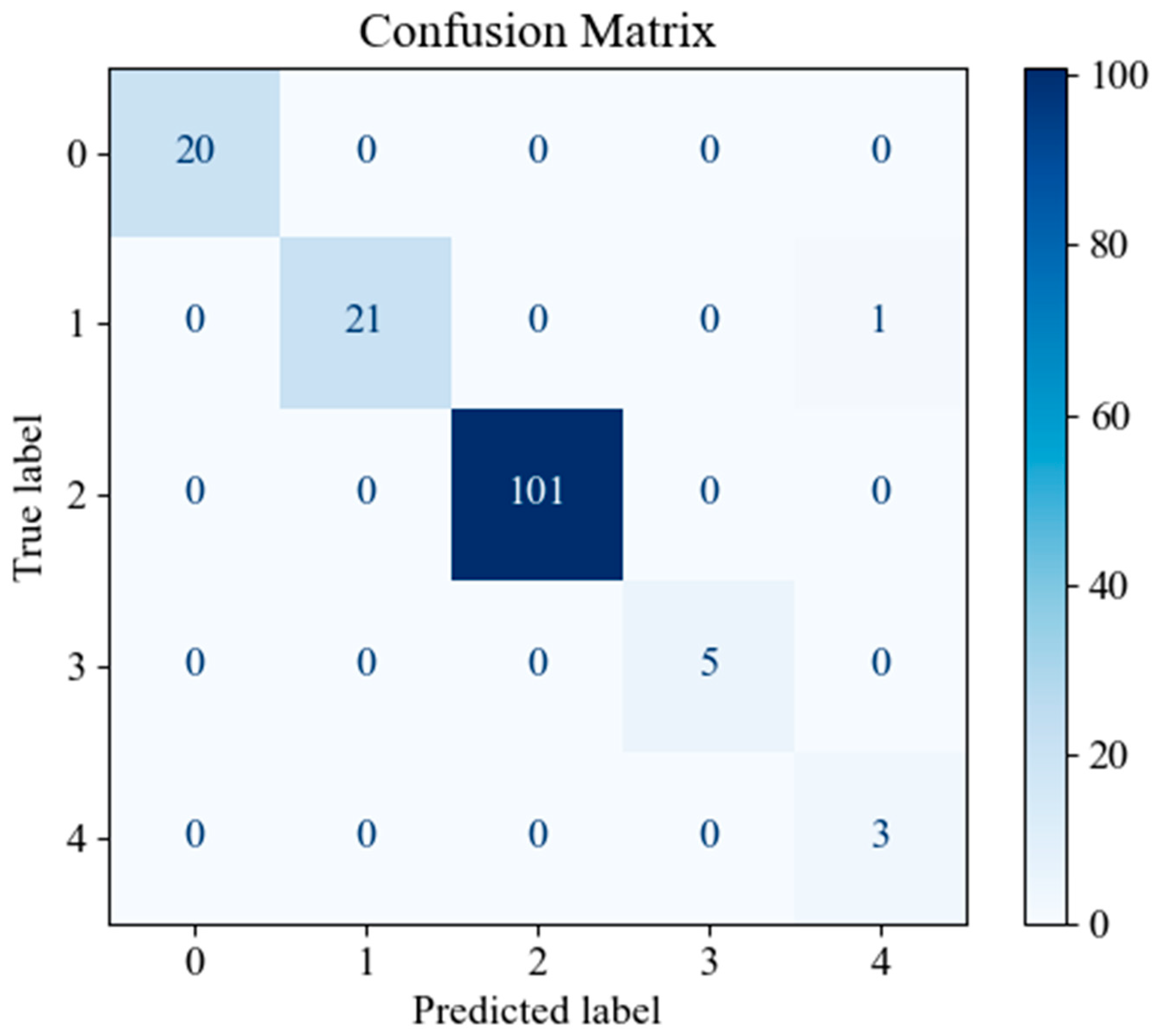
In order to assess the predictive performance of the SHAP-GAN network proposed in this study on the ovarian cancer dataset, a confusion matrix and a Receiver Operating Characteristic (ROC) curve were both generated. The confusion matrix, depicted in Figure 10, is presented as a 5 × 5 grid, with each cell corresponding to one of the five types of ovarian cancer in the dataset, highlighting the multi-class classification aspect of the task. The diagonal elements of the matrix signify accurately classified samples. 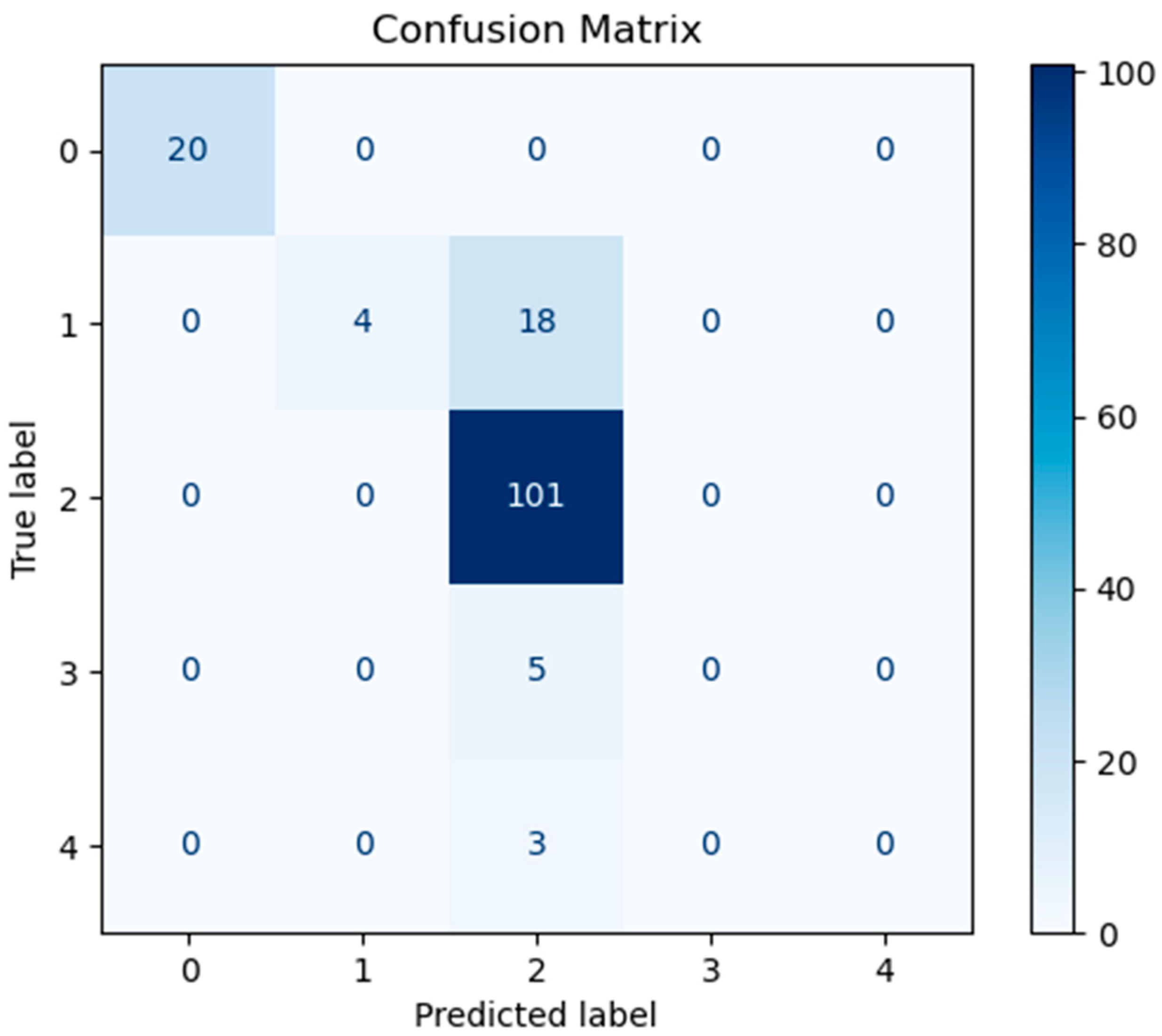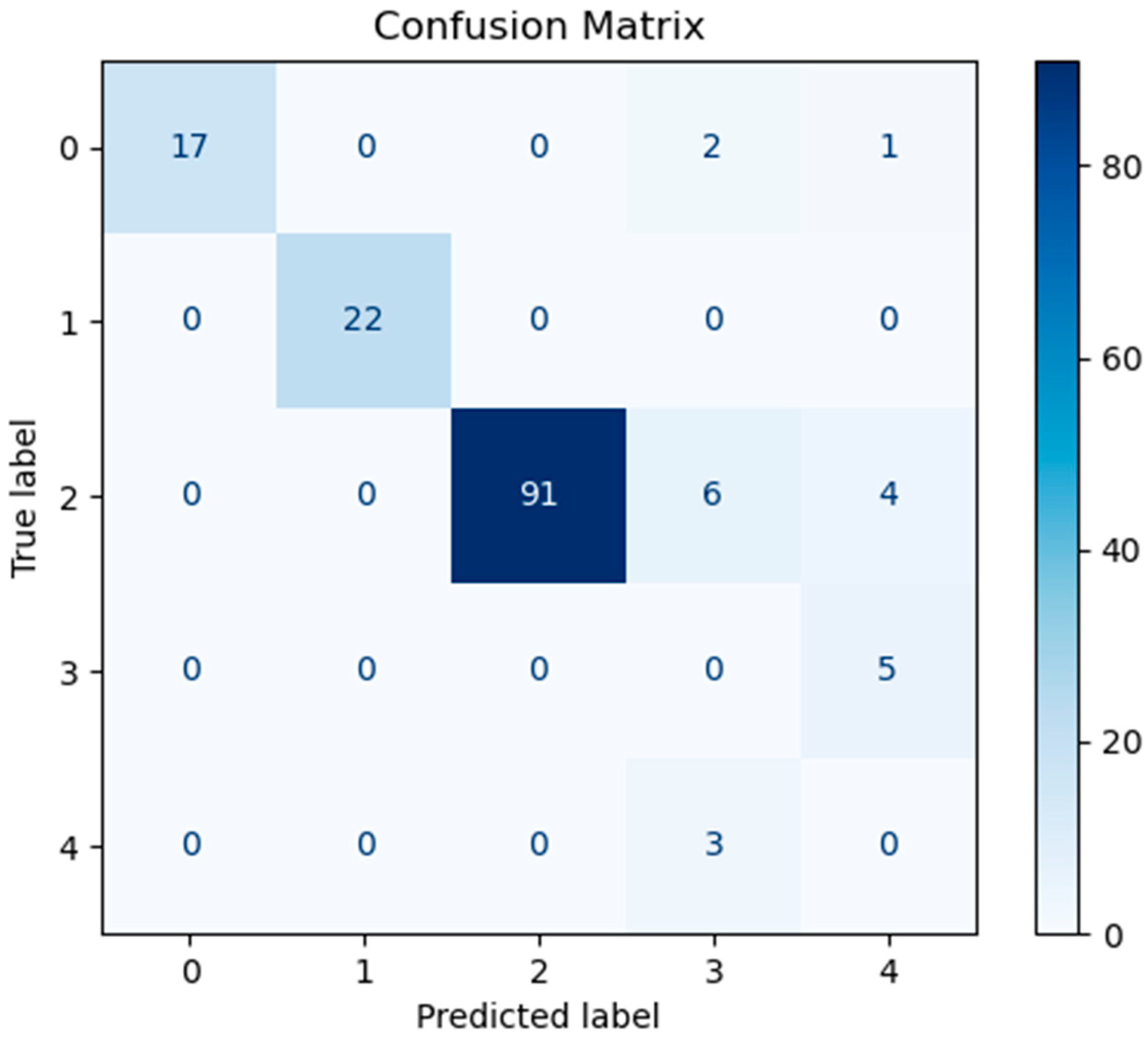Figure 10, Figure 11, and Figure 12 represent the confusion matrices of the SVM, LR, and XGBoost models within the baseline model, respectively. These matrices reveal that a significant number of samples were misclassified by these traditional models, indicating limitations in their classification accuracy. SVM tends to be biased towards the majority class when handling imbalanced data. Since classes 3 and 4 have fewer samples, SVM may focus on the more common classes during training, leading to misclassification of the minority classes. Logistic Regression (LR) assumes a linear relationship between features and classes. However, in real gene expression data, the relationship between features and classes may be highly non-linear. Logistic Regression fails to capture these non-linear relationships, which leads to poor performance on complex datasets. In high-dimensional datasets, XGBoost is prone to overfitting, especially when the depth of trees or the number of iterations is set too high. Even though XGBoost has strong generalization ability, if the model complexity is not well-controlled during training, it may result in reduced performance on the test set. However, the confusion matrix of the SHAP-GAN network model presented in Figure 13 demonstrates a substantial improvement in classification performance. Specifically, classes 0, 2, 3, and 4 have been perfectly classified, with all instances correctly identified. The only misclassification observed is one instance of class 1, which was incorrectly assigned to class 4. This result highlights the superior performance of the SHAP-GAN network model in handling the classification task compared to the baseline models.

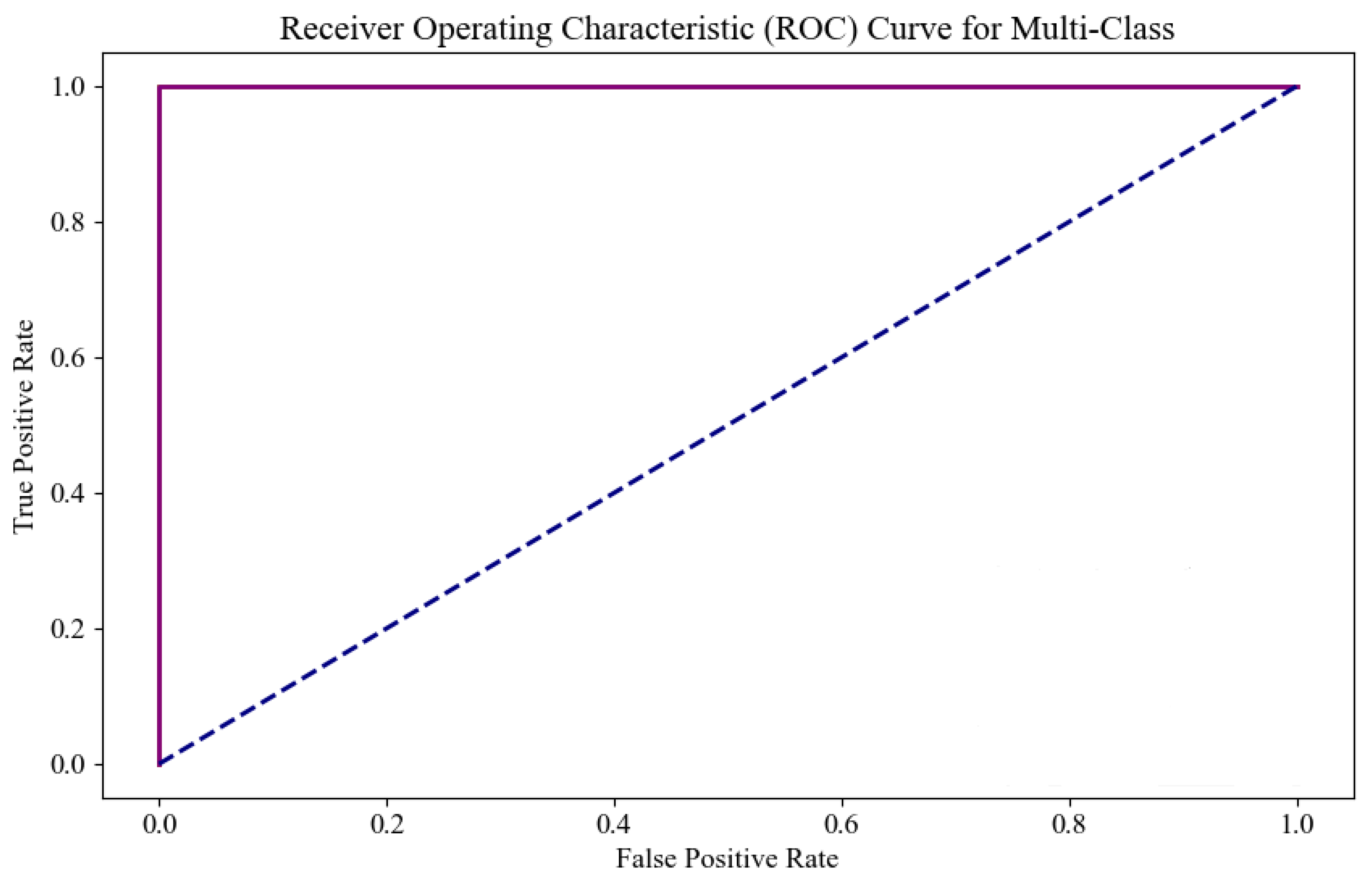
Figure 14 shows the ROC curve of the model on this dataset, where the x-axis represents the false positive rate and the y-axis represents the true positive rate. As the decision threshold changes, the values of TPR and FPR also change, forming a curve that reflects the model’s classification performance at different thresholds. In the ROC curve, the area under the curve (AUC) indicates the model’s classification ability, with the AUC value ranging from 0 to 1. The closer the AUC is to 1, the stronger the model’s classification ability. An AUC of 0.5 indicates that the model has no classification ability. According to the ROC curve, the AUC for classes 0, 2, 3, and 4 is 1, indicating perfect classification performance. While the AUC for class 3 is also 1, as shown in Figure 11, its curve slightly deviates from ideal classification. This is because the AUC is calculated by evaluating the model’s classification rate across all classes, and the limited sample size for class 1 means the model may over-rely on a small number of samples. As a result, even if the model only predicts a few class 3 samples, it may still achieve a high AUC. This issue is commonly known as the “class imbalance” problem, where a high AUC for minority classes may not truly represent the model’s classification performance for those classes. Therefore, while the AUC is 1, it does not imply that the model’s prediction capability for class 3 is entirely reliable, and there may be a deviation in the actual performance. Overall, the results in Figure 11 provide strong evidence of the excellent predictive performance of the algorithm proposed in this study for ovarian cancer classification tasks, demonstrating its robust identification ability across multiple classes.

To better validate the impact of SHAP-GAN on the overall model prediction accuracy, an ablation study was conducted, and the experimental results are shown in

Table 4. The ablation experiment of the model for the ovarian cancer dataset.

Method	Classification Accuracy (%)
ACGAN + XGBoost	98.00
Feature selection + ACGAN + XGBoost	98.68
The proposed SHAP-GAN network	99.34

. As can be seen from Table 4, if no feature selection process is conducted and only ACGAN oversampling is performed, the overall accuracy of the model is only 98%. If the ACGAN network generates data without the guidance of the SHAP module, the model accuracy is 98.68%. Therefore, the SHAP-GAN module demonstrates excellent performance in the early diagnosis of ovarian cancer using the gene dataset.

From the experimental results, it can be seen that using SHAP values to guide the weight adjustment of the ACGAN generator can significantly improve the quality and diversity of the generated samples, thereby enhancing the overall performance of the model. SHAP values provide global and local explanations of feature importance, enabling the generator to identify which features contribute the most to the classifier’s decisions. This allows the generator to specifically optimize the creation of these key features. This method not only prevents the generator from blindly producing low-quality samples but also ensures that the generated samples better match the feature distribution of the target class, enhancing the realism and diversity of the samples. Moreover, by adjusting the generator’s weights, the generator can more efficiently explore the feature space, avoiding mode collapse and producing more meaningful samples for the classifier. Ultimately, these high-quality generated samples can be used for data augmentation, significantly improving the classifier’s generalization ability and performance. This is especially evident in imbalanced and high-dimensional datasets, such as the ovarian cancer gene dataset, where the impact is particularly notable. This research can notably improve classification accuracy, offering direct advantages for patients. It also has the potential to uncover previously unnoticed features in disease progression or response to treatments, thereby enriching the scientific community’s comprehension of ovarian cancer.

5. Conclusions

This study proposes a novel SHAP-GAN network for ovarian cancer diagnosis, integrating the strengths of GANs in generating realistic samples with the interpretability of SHAP values. This approach produces synthetic samples that are both visually convincing and medically meaningful, addressing the challenges of high dimensionality and data imbalance in ovarian cancer datasets. The SHAP-GAN network comprises three key components: feature selection, data augmentation, and a predictive classifier, which collectively enhance the predictive accuracy and interpretability of the model.

Experimental results demonstrate that the SHAP-GAN network outperforms traditional oversampling methods by generating more diverse and representative synthetic samples while avoiding the noise and redundancy often introduced by conventional techniques. By incorporating SHAP’s interpretability, the network not only improves the classifier’s prediction accuracy for rare categories but also provides medically meaningful feature attributions, offering clear and interpretable biomarkers for ovarian cancer diagnosis. Furthermore, the SHAP-GAN network leverages SHAP’s feature importance evaluation to generate synthetic samples that are both representative and reasonable, avoiding issues of overfitting or excessive randomness. This enhances the model’s generalization ability, stability, and accuracy, as evidenced by its impressive accuracy rate of 99.34% on the ovarian cancer dataset.

While these results are promising, the primary goal remains the development of a practical tool to assist healthcare professionals in clinical settings. To this end, future work will focus on validating the algorithm’s feasibility using more representative clinical datasets from diverse regions, guided by clinical experts, and employing multiple evaluation criteria to mitigate diagnostic differences and selection bias across populations. Additionally, long-term clinical follow-up studies will be conducted to assess the model’s dynamic adjustment capabilities and its ability to adapt to patients’ evolving conditions over time. The efforts put into enhancing the clinical applicability of the SHAP-GAN network are expected to support personalized treatment strategies and improve outcomes for ovarian cancer patients.