Abstract
This paper considers difference equations with continuous time, piecewise linear delay functions, and oscillatory coefficients. We present new conditions on the coefficients that provide the oscillatory property of the solutions of the considered difference equations. The given criteria are compared to the existing oscillatory conditions in the literature using examples.
Keywords:
difference equation; continuous time; piecewise linear delay function; oscillating coefficients; oscillatory solutions MSC:
39A21; 39A10
1. Introduction
Applications of delay difference equations with continuous time, and evidence of their importance, can be found in mechanical and electrical systems, as is stated in [1], as well as in modeling distributed chaos, as is pointed out in [2,3]. Analyses of the oscillatory properties of solutions of delay difference equations with continuous time were the subject of the papers [4,5,6,7,8] and also the papers [9,10,11], but in the form of special cases of iterative functional equations. The literature on the oscillatory properties of solutions of differential and discrete difference equations can be divided into two groups: one with nonnegative or positive coefficients and the other with oscillatory coefficients. Studies on the oscillatory properties of solutions of differential equations with nonnegative coefficients can be found, for example, in the papers [12,13,14], while those with oscillating coefficients are found in [15,16]. For example, the papers [13,17,18,19,20,21] are devoted to discrete difference equations with positive coefficients and oscillatory coefficients, respectively. Since many papers dealing with difference equations with continuous time have analyzed equations with positive or nonnegative coefficients (all of those mentioned above) but only (to the best of our knowledge) the paper [22] has considered oscillatory coefficients, our aim is to expand the set of known oscillatory conditions for solutions of delay difference equations with continuous time and oscillatory coefficients.
In this paper, we continue the research from our paper [22], so we analyze the oscillatory property of the solutions of the delay difference equation
where , , and . For , is a piecewise continuous and oscillatory function, but the delay argument is in the form
where the function is piecewise constant. Also, the delay arguments have the following properties:
and
We present two oscillatory criteria and compare them to the oscillatory conditions in [22]. The comparison, using the presented examples, shows that there is a set of difference equations for which our new oscillatory criteria prove that their solutions oscillate, while the known criteria are not applicable to them. This confirms that we have extended the set of difference equations in form (1) for which conditions verifying their oscillatory properties exist.
A solution of delay difference Equation (1) is a real-valued function x defined on the interval , with
that satisfies Equation (1). If a solution of (1) changes the sign on the interval for any s, it is oscillatory. Otherwise, it is nonoscillatory. As in [7], for any bounded real-valued function defined on the interval , there exists a unique solution x of (1) that satisfies the initial condition , since it can be represented by
As a standard, for any , , and a real-valued function f,
and
2. The New Oscillation Criteria
We define a real-valued function
and
These functions have the following properties:
For more details and illustrations with examples, see [22].
First, we give the following lemma.
Lemma 1.
If there exists a sequence of disjoint intervals with the properties for every ,
and for some ,
then there exists a sequence such that and
but
Proof.
Now, we prove an auxiliary lemma.
Lemma 2.
Proof.
Due to the definition of limit inferior and (20), for an arbitrary , so for ,
Hence,
and consequently,
Since , condition (19) ensures that for every and . Besides this, (18), (19), and (23) ensure that the sequence of intervals satisfies the conditions of Lemma 1 with . Therefore, there exists a sequence such that ,
According to (22),
so using (24), we obtain
Property (10) secures that .
Since x is a nonoscillatory solution of (1), without loss of generality, we can assume that
For every , property (11) ensures that for every , ; thus, , so (1), (19), and (27) provide
i.e.,
Consequently,
Also, (11) ensures that for every . Therefore, (9) and (28) provide that
Summing up (1) from to , we obtain
Hence, according to (25),
Similarly, summing up (1) from to , we obtain
Therefore, (26) implies
Combining the inequalities (30) and (31), we obtain
i.e.,
Since ,
Given that and , we have
Consequently,
Since (32) holds for an arbitrarily small , this implies (21). The proof of the lemma is complete. □
Now, we are ready to formulate and prove a new criterion that shows that all of the solutions of the observed difference equation are oscillatory.
Theorem 1.
Proof.
As in the proof of the previous lemma, for , and denote the intervals and , respectively.
Supposing the opposite, let the function be a nonoscillatory solution of (1). Without loss of generality, we can assume that
Therefore, (11), (1), (19), and (34) imply
Consequently, for every ,
Since (11) ensures that for every , (9) and (35) provide
For any , summing up (1) from to , then given that and applying (19) and (36), afterwards, according to (19), (10), and (35), we have
Dividing the obtained inequality by , which is positive, we obtain
i.e.,
Hence,
Applying (21) from Lemma 2, we have
which is a contradiction to condition (33). The proof of the theorem is complete. □
Due to the following corollary, the nonnegativity of the coefficients in the definition of and the coefficients in condition (33), combined with property (10), yield the conclusion that for , there is no need to check the condition (33).
Corollary 1.
Proof.
Notice that the oscillatory conditions in Theorem 1 and Corollary 1 require nonnegativity of the coefficients in the disjoint intervals and do not use the intervals where the coefficients are negative. Therefore, the presented oscillatory conditions can be applied to establishing the oscillatory property of solutions of the difference equations in form (1) with oscillating coefficients, but they also apply to equations with positive coefficients.
3. Examples and Comparisons
The following examples illustrate the presented conditions for oscillatory solutions of the observed difference equation. For the first two examples, the oscillatory conditions from Theorem 1 are satisfied, but the oscillatory conditions from Corollary 1 and the oscillatory conditions from [22] are not fulfilled. The last example shows the application of the oscillatory conditions from Corollary 1 to a delay difference equation with unbounded delays. Moreover, the oscillatory conditions from [22] are not satisfied for that example either.
Theorem 2
([22] (Theorem 2.2)). For the functions τ and defined by (6) and (7), respectively, assume that there exists a sequence of real numbers such that condition (17) holds and the intervals of the sequence are nonempty, disjoint, and contained in . If, in addition,
and
then all of the solutions of (1) are oscillatory.
Theorem 3
([22] (Theorem 2.3)). For the functions τ and defined by (6) and (7), respectively, assume that there exists a sequence of real numbers such that condition (17) holds and the intervals of the sequence are nonempty, disjoint, and contained in . If, moreover,
and there exists a real number such that
then all of the solutions of (1) are oscillatory.
Example 1.
Here, , and ; thus, , and . Therefore, , and . For the sequence of real numbers such that ,
so, for every ,
This means that conditions (17)–(19) are satisfied with
Due to and
condition (33) is also fulfilled; thus, all of the conditions of Theorem 1 are satisfied, and therefore all of the solutions of Equation (43) are oscillatory.
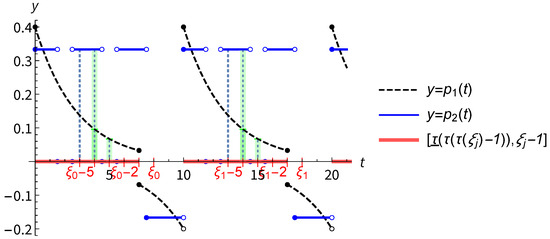
Consider the difference equation
where the functions and are periodic, with the basic period 10, such that
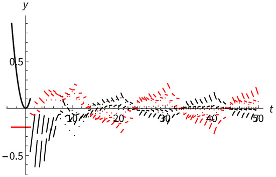
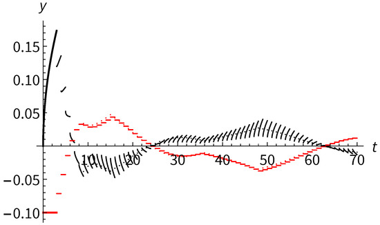
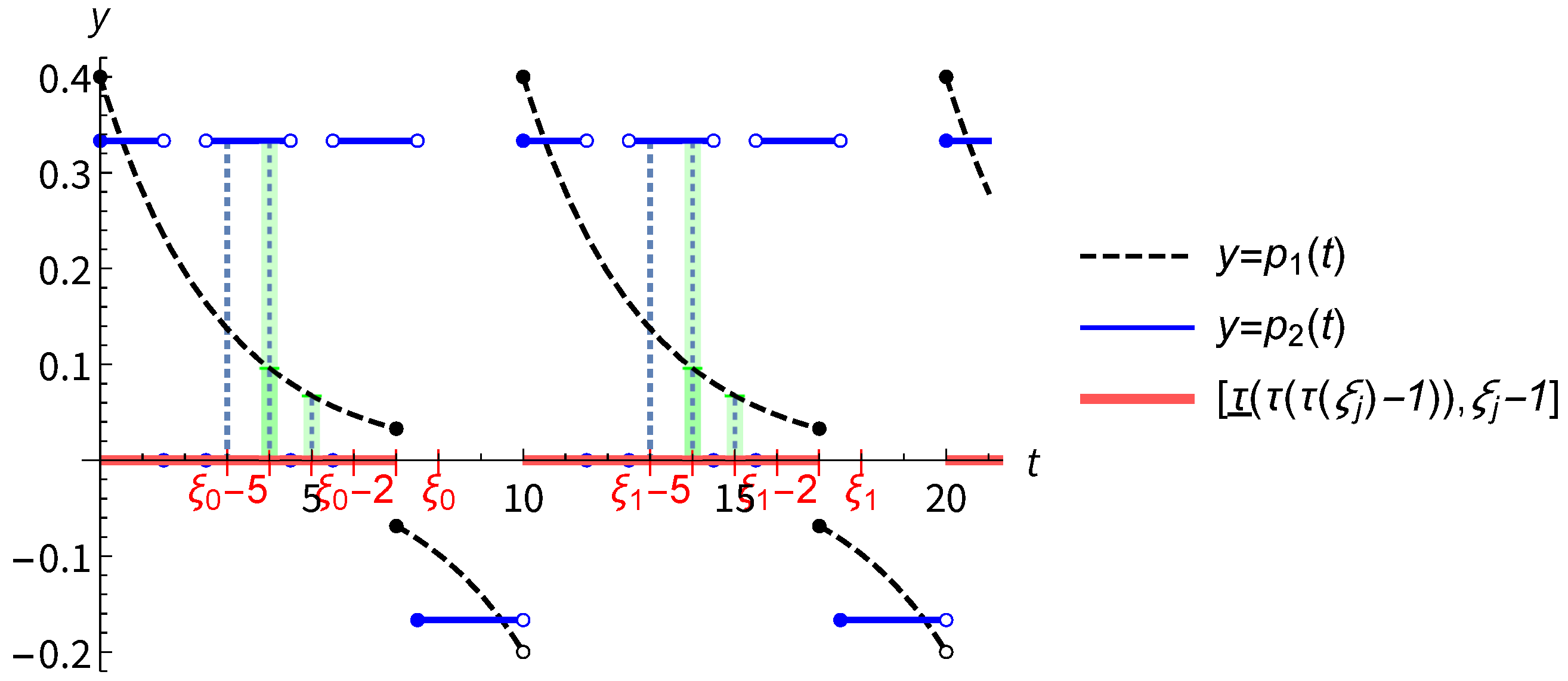
The graphs of the functions and , the intervals , and the relevant points from conditions (20) and (33) are presented in Figure 1. Figure 2 shows the graphs of some of the solutions of Equation (43).
Figure 2.
The graphs of solutions of Equation (43) with initial functions (black curve) and (red curve), .
The conditions of Theorem 3 cannot be fulfilled since the length of the intervals of condition (41) are expanding as j increases, but the functions and are nonnegative only at the interval with a length of 7. Therefore, the oscillatory conditions of Theorem 3 cannot be satisfied.
Example 2.

The conditions of Theorem 1 are satisfied for equation
with
and
so all of the solutions of Equation (44) are oscillatory.
Namely, , and ; thus, , and . Therefore, , and . For every ,
For the sequence of real numbers such that ,
so for ,
Hence, conditions (17)–(19) are satisfied, and
Since and
condition (33) also holds, so all of the conditions of Theorem 1 are fulfilled.
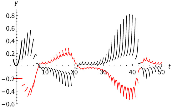
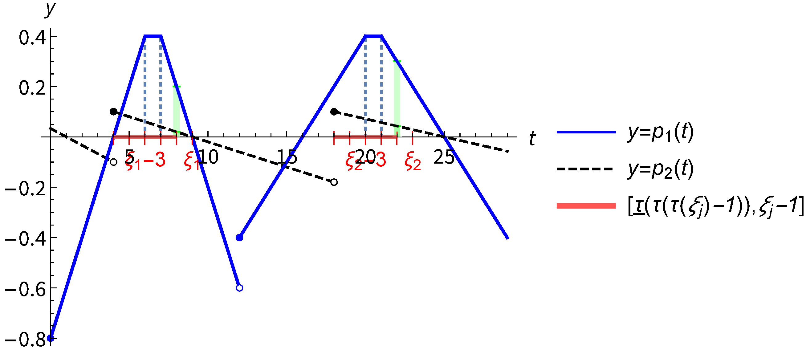
The graphs of the functions and , the intervals , and the relevant points from conditions (20) and (33) are presented in Figure 3. Figure 4 shows graphs of some of the solutions of Equation (44).
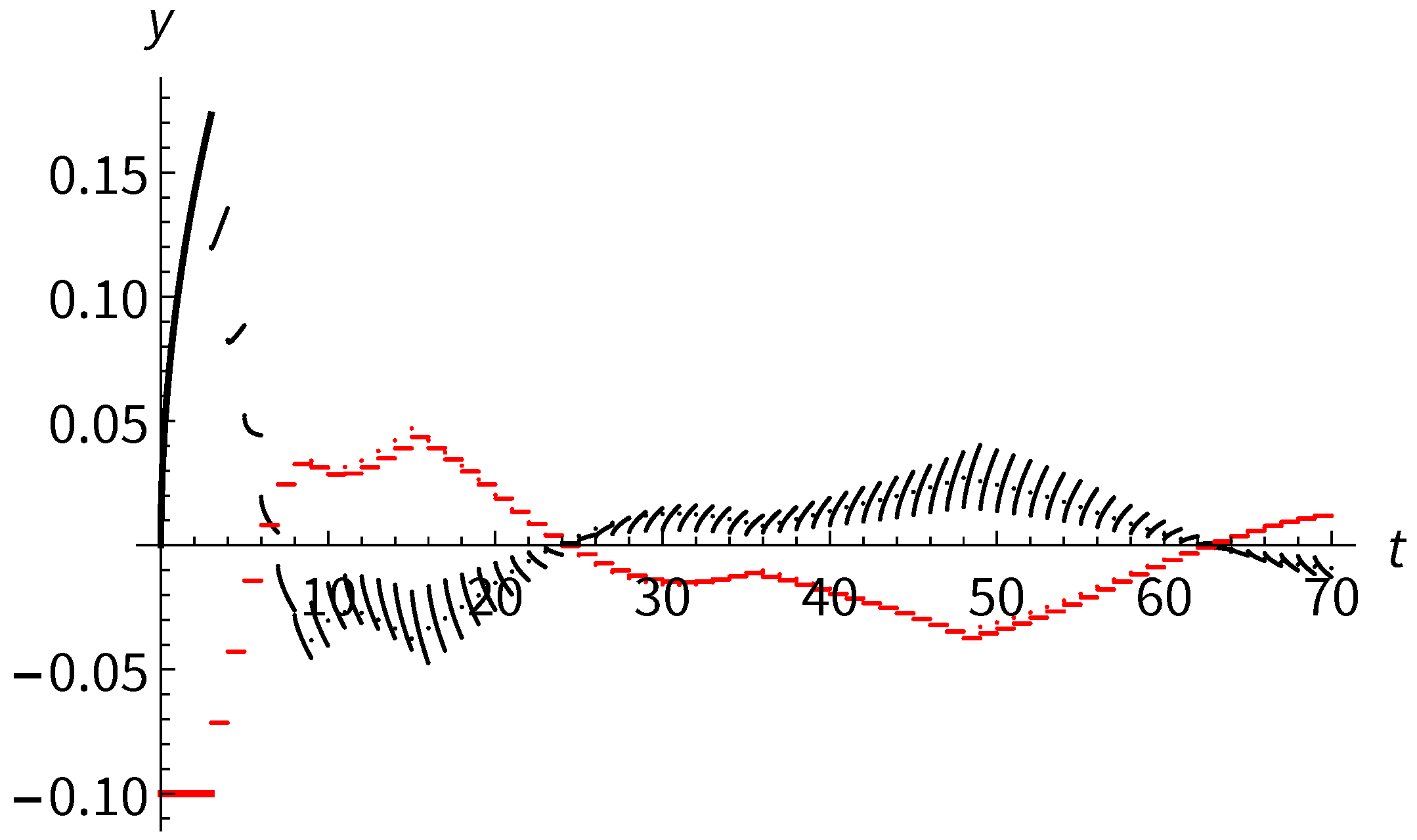
Figure 4.
The graphs of solutions of Equation (44) with initial functions (black curve) and (red curve), .
Example 3.
Consider the difference equation
with
and
where denotes the integer part.
The delay functions, and , are unbounded but satisfy conditions (3) and (4). and ; thus, for the sequence of real numbers such that ,
Therefore,
so conditions (17)–(19) are satisfied. Equally,
implying that
Hence,
Consequently, the conditions of Corollary 1 are satisfied, so all of the solutions of Equation (45) are oscillatory.
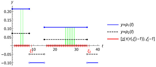
The graphs of the functions and , the intervals , and the relevant points from condition (20) are presented in Figure 5. Figure 6 shows graphs of some of the solutions of Equation (45).
Figure 5.
The graphs of the functions and , the intervals , and the points from Example 3. The green lines represent the values in sums from condition (20).
Figure 6.
The graphs of solutions of Equation (43) with initial functions (black curve) and (red curve), .
The oscillatory conditions of Theorem 2 cannot be satisfied since for any sequence of real numbers such that condition (39) is fulfilled, for some , so
Hence,
Given that ,
and therefore
Since the intervals of sequence are disjoint, implies that , so inequality (46) gives
Consequently, condition (40) cannot be fulfilled.
The conditions of Theorem 3 also cannot be fulfilled since there is no sequence of real numbers such that condition (41) is satisfied. Namely, according to condition (41), there is a sequence of real numbers such that
for some . The length of the interval is expanding as n increases, and the length of the interval is . Even for ,
so the length of the interval is . Since for every , the condition (47) cannot be fulfilled for any integer and . Hence, the oscillatory conditions of Theorem 3 cannot be satisfied.
4. Conclusions
Our study of the oscillatory properties of the solutions of first-order difference equations with continuous time, piecewise linear delay functions, and oscillatory coefficients has led us to a new condition that ensures the oscillatory solutions. According to the proposed results, the oscillatory property of all solutions of the considered difference equation is ensured with sufficiently positive coefficients in the equation in the sense that the sum of the values of the coefficients defined by in (20) is in the interval . For , the oscillatory property of all solutions is ensured when condition (33) is fulfilled.
We have shown, using examples, that there are difference equations for which the previously known oscillatory conditions for the same types of difference equations are not applicable, but the proposed criteria are satisfied. Therefore, we have extended the set of difference equations with oscillatory coefficients for which conditions verifying their oscillatory properties exist.
Author Contributions
Conceptualization: G.E.C. and H.P. Methodology: H.P. and A.R. Investigation: H.P. and A.R. Writing—original draft preparation: A.R. Writing—review and editing: G.E.C., H.P., and A.R. All authors have read and agreed to the published version of the manuscript.
Funding
This research received no external funding.
Data Availability Statement
No new data were created or analyzed in this study. Data sharing is not applicable to this article.
Acknowledgments
We thank our anonymous referees for their valuable comments and help.
Conflicts of Interest
The authors declare no conflicts of interest.
References
- Sharkovsky, A.N.; Maistrenko, Y.L.T.; Romanenko, E.Y. Difference Equations and Their Applications; Ser. Mathematics and Its Applications 250; Springer: Dordrecht, The Netherlands, 1993. [Google Scholar] [CrossRef]
- Romanenko, O. Continuous-time difference equations and distributed chaos modelling. Math. Lett. 2022, 8, 11–21. [Google Scholar] [CrossRef]
- Sharkovsky, A.N. Chaos from a time-delayed Chua’s circuit. IEEE Trans. Circuits Syst. I Fund. Theory Appl. 1993, 40, 781–783. [Google Scholar] [CrossRef]
- Braverman, E.; Johnson, W.T. On oscillation of difference equations with continuous time and variable delays. Appl. Math. Comput. 2019, 355, 449–457. [Google Scholar] [CrossRef]
- Chatzarakis, G.E.; Péics, H.; Rožnjik, A. Oscillations in difference equations with continuous time caused by several deviating arguments. Filomat 2020, 34, 2693–2704. [Google Scholar] [CrossRef]
- Karpuz, B.; Öcalan, Ö. Discrete approach on oscillation of difference equations with continuous variable. Adv. Dyn. Syst. Appl. 2008, 3, 283–290. [Google Scholar]
- Ladas, G.; Pakula, L.; Wang, Z. Necessary and sufficient conditions for the oscillation of difference equations. Panam. Math. J. 1992, 2, 17–26. [Google Scholar]
- Zhang, B.G.; Yan, J.; Choi, S.K. Oscillation for difference equations with continuous variable. Comput. Math. Appl. 1998, 36, 11–18. [Google Scholar] [CrossRef]
- Nowakowska, W.; Werbowski, J. Conditions for the oscillation of solutions of iterative equations. Abstr. Appl. Anal. 2004, 2004, 543–550. [Google Scholar] [CrossRef]
- Shen, J.; Stavroulakis, I.P. An oscillation criteria for second order functional equations. Acta Math. Sci. Ser. B Eng. Ed. 2002, 22, 56–62. [Google Scholar] [CrossRef]
- Zhang, B.G.; Choi, S.K. Oscillation and nonoscillation of a class of functional equations. Math. Nachr. 2001, 227, 159–169. [Google Scholar] [CrossRef]
- Attia, E.; El-Matary, B. New explicit oscillation criteria for first-order differential equations with several non-monotone delays. Mathematics 2023, 11, 64. [Google Scholar] [CrossRef]
- Braverman, E.; Karpuz, B. On oscillation of differential and difference equations with non-monotone delays. Appl. Math. Comput. 2011, 218, 3880–3887. [Google Scholar] [CrossRef]
- Kiliç, N.; Öcalan, Ö. A new oscillation result for nonlinear differential equations with nonmonotone delay. Miskolc Math. Notes 2023, 24, 841–851. [Google Scholar] [CrossRef]
- Fukagai, N.; Kusano, T. Oscillation theory of first order functional differential equations with deviating arguments. Ann. Mat. Pura Appl. 1984, 136, 95–117. [Google Scholar] [CrossRef]
- Tang, X. Oscillation of first order delay differential equations with oscillating coefficients. Appl. Math. J. Chin. Univ. Ser. B 2000, 15, 252–258. [Google Scholar] [CrossRef]
- Attia, E.R.; Alotaibi, S.M.; Chatzarakis, G.E. New oscillation criteria for first-order difference equations with several not necessarily monotonic delays. J. Appl. Math. Comput. 2024, 70, 1915–1936. [Google Scholar] [CrossRef]
- Koplatadze, R.; Khachidze, N. Oscillation criteria for difference equations with several retarded arguments. J. Math. Sci. 2020, 246, 384–393. [Google Scholar] [CrossRef]
- Berezansky, L.; Chatzarakis, G.E.; Domoshnitsky, A.; Stavroulakis, I.P. Oscillations of difference equations with several oscillating coefficients. Abstr. Appl. Anal. 2014, 2014, 392097. [Google Scholar] [CrossRef]
- Yan, W.; Yan, J. Comparison and oscillation results for delay difference equations with oscillating coefficients. Int. J. Math. Math. Sci. 1996, 19, 171–176. [Google Scholar] [CrossRef]
- Yu, J.S.; Tang, X.H. Sufficient conditions for the oscillation of linear delay difference equations with oscillating coefficients. J. Math. Anal. Appl. 2000, 250, 735–742. [Google Scholar] [CrossRef]
- Chatzarakis, G.E.; Péics, H.; Rožnjik, A. Oscillations of deviating difference equations with continuous time and oscillatory coefficients. J. Differ. Equ. Appl. 2023, 29, 682–700. [Google Scholar] [CrossRef]


Disclaimer/Publisher’s Note: The statements, opinions and data contained in all publications are solely those of the individual author(s) and contributor(s) and not of MDPI and/or the editor(s). MDPI and/or the editor(s) disclaim responsibility for any injury to people or property resulting from any ideas, methods, instructions or products referred to in the content. |
© 2025 by the authors. Licensee MDPI, Basel, Switzerland. This article is an open access article distributed under the terms and conditions of the Creative Commons Attribution (CC BY) license (https://creativecommons.org/licenses/by/4.0/).