Abstract
This study investigates extremal solutions for fractional-order delayed difference equations, utilizing the Caputo nabla operator to establish mild lower and upper approximations via discrete fractional calculus. A new approach is employed to demonstrate the uniform convergence of the sequences of lower and upper approximations within the monotone iterative scheme using the summation representation of the solutions, which serves as a discrete analogue to Volterra integral equations. This research highlights practical applications through numerical simulations in discrete bidirectional associative memory neural networks.
Keywords:
Caputo-type fractional difference; nabla fractional sum; constant delay; mild upper and lower solutions MSC:
34A08; 34A12
1. Introduction
Fractional derivatives offer precise modeling of diverse natural phenomena [1,2]. Despite limited exploration, fractional difference equations—discrete analogs to continuous fractional dynamical systems—are increasingly being studied, particularly for delay components. The existence and uniqueness of time-delayed nabla fractional systems are established in [3,4]. For a detailed overview of discrete fractional calculus, refer to monograph [5]. In engineering applications like missile guidance and robotics, maintaining system trajectories within limits prevents control loss or threshold breaches [6]. The study of dynamic behaviors under external influences is detailed in generalized oscillator models [7]. The monograph [8] thoroughly examines the existence and stability of solutions for fractional difference equations, addressing delays and impulsive effects using fixed point theorems and upper–lower approximations. The study [9] investigates Ulam stability in delay fractional difference equations using Gronwall’s discrete inequality, enhancing understanding in neural networks. In the research [10], memory effects in neural networks are addressed through variable-order fractional discrete-time recurrent neural networks, including applications of fractional discrete-time neural network associated with standard Hopfield-type fractional neural networks:
or
where represents the state vector; , with , denotes the state feedback coefficients; is the network’s interconnection matrix; is the activation function; and I indicates the constant external input. Short memory models are proposed with stability analysis via fixed point techniques, and the applications extend to chaos control and diffusion modeling.
The aforementioned studies emphasize the pivotal role of fractional calculus in modeling neural network memory, serving as a primary motivation for this research aimed at identifying discrete analogs for these systems. Previous numerical solutions have encountered challenges due to cumulative errors from infinite-memory effects, numerical truncation, and convergence issues. To address these challenges effectively within applications like bidirectional associative memory neural networks, this study proposes utilizing discrete fractional calculus on isolated time scales.
Recent studies on Caputo, Riemann–Liouville, and impulsive differential equations with generalized proportional derivatives utilize upper–lower solutions as well as monotone iterative techniques [11,12,13,14,15] and for Caputo-type fractional nabla difference equations [16]. The Banach–Schauder fixed point theorem confirms solution existence under nonlinear delta scenarios with delays/impulses [17]. Challenges in fractional differential/difference equations arise from non-linearity and delays. Various methods combine upper–lower solutions with monotone iterative techniques. One approach uses explicit formulas for linear inhomogeneous equation approximation [12]; supposing Lipschitz condition, another selects analytic properties of functions within problem statements specific to difference contexts [13,16]. This article examines a Caputo-type fractional nabla difference equation () using the sum of two monotonic functions on the right-hand side. Approximation results utilize summation equations, defining mild extremal solutions according to the methods of Agarwal et al. [13], establishing sufficient conditions for monotonicity and uniform convergence. In related work, [18] presents key insights into the overconvergence of functional series.
In the present study, a monotone iterative method utilizing coupled mild lower and upper solutions is employed to approximate the exact solution of nabla fractional delayed difference equations. The impact of fractional operator orders is examined through numerical simulations. Integral representations are essential for analyzing solution behavior and stability in fractional differential equations or systems with delays [19,20]. Discrete counterparts are utilized within iterative algorithms in this study. Instability often arises from undetected disturbances and ineffective management due to time delays. Consequently, significant efforts have been dedicated by scientists and engineers to studying the stability of fractional neural networks with time delays. For asymptotic stability in nonlinear nabla fractional difference equations with bounded time delays, refer to [21]. Applications for variable-order systems are discussed in [22]. In [23], sufficient conditions for existence, uniqueness, and uniform stability of non-trivial solutions in discrete fractional-order neural networks with leakage delay were established using discrete fractional calculus along with mathematical inequalities and fixed point theorems.
This research addresses the following aspects:
- (I)
- The introduction of an iterative method employing mild upper and lower solution approximations for Caputo fractional nabla delayed difference equations.
- (II)
- The establishment of a novel analytical framework demonstrating uniform convergence of successive approximation sequences, grounded in fundamental real and functional analysis principles.
- (III)
- The demonstration of the algorithm’s practical utility within Bidirectional Associative Memory (BAM) neural networks, demonstrating its effectiveness in improving network performance through innovative applications.
The subsequent sections of this paper are structured as follows: Section 2 explains foundational concepts and definitions related to discrete fractional calculus relevant to our study. Section 3 is dedicated to applying the outlined methodology for deriving the main results. In Section 4, illustrative examples with computer simulations are presented.
2. Background of the Main Results
2.1. Fractional Difference Calculus: Definitions
This section explains the basic concepts of the -order Caputo-type nabla fractional operator. Let and T be integers. The following sets will be utilized:
Definition 1
(Def. 2.2., [24]). Let denote the backward jump operator. Then, the (nabla) left fractional sum of order is defined by
where is the (generalized) rising function with , and
Lemma 1
(Lemma 2.2., [25]). Assume that the following properties of the rising function are well defined:
- (i)
- (ii)
- If then
- (iii)
- If then
Theorem 1
(Th. 2.4., [25]). Consider and It can be concluded that
Definition 2
(Def. 3.117, [5]). Let The Caputo fractional nabla difference for is defined as follows:
by convention .
Theorem 2
(Th. 3.119, [5]). Let . For , it can be concluded that
2.2. Problem Set Up and Preliminaries
We examine the initial value problem () for nonlinear with a constant delay, expressed as follows:
where are continuous in their second and third variables, with u being non-decreasing and w non-increasing, with respect to these variables on . Additionally, , where and denotes the Caputo fractional difference of order .
Lemma 2
(Lemma 1, [26]). A function is a solution to Equation (1) if, and only if, the following representation holds
Remark 1.
Previous studies, specifically [26,27] have provided the representation denoted by (2). It serves as a fundamental basis for our main results, exploring cases without guaranteed unique solutions. Such inquiries into equations similar to Equation (1), with arbitrary nonlinear functions on the right-hand side, have been examined in [26] for the discrete domains and in [11,27] for the continuous domains.
The exposition below requires definitions from real and functional analysis [28,29].
Definition 4.
Suppose that is a sequence of functions .
- (i)
- Pointwise Convergence: A sequence is said to converge pointwise on S if, for every , the limit
- (ii)
- Uniformly Cauchy: The sequence is uniformly Cauchy if, for every , there exists such that whenever for any in
Let represent the space of all real sequences defined over the positive integers, each bounded with respect to the supremum norm. It is evident that is a Banach space under this norm.
Define the set
Theorem 3.
Let The sequence of real function is uniformly Cauchy on S if, and only if, it converges uniformly on S.
Remark 2.
An analogy exists between uniform and pointwise convergence, similar to the relationship between continuous and uniformly continuous functions. Uniform versions require a single parameter or that applies universally across the domain, while pointwise definitions allow parameters to vary with each specific point. This distinction highlights a fundamental difference in controlling variation across different types of convergence and continuity.
2.3. Initial Assessments on Mild Extremal Solutions
This section delineates mild upper and lower solutions for (1). For detailed information on mild solution techniques, see [12,13]. The authors examine scalar differential equations with Riemann–Liouville derivatives, addressing both delayed and non-delayed cases. Known for initial point discontinuities, these derivatives pose challenges that mild solutions mitigate. It is established that a mild solution may lack an existing fractional derivative, paralleling discrete case observations [30], warranting further study of Riemann–Liouville difference equations. For insights on Caputo-type equations, see [31].
Definition 5.
Let . The functions are termed coupled mild lower–upper solutions () of Type I for Equation (1) if they satisfy
Remark 3.
For a variety of lower/upper solutions of (1), see Def. 5 in [11], and for a mild lower/upper solutions, refer to Def 4.7 in [13]. The current work focuses on a of Type I.
Definition 6.
A function is called a mild minimal (or maximal) solution of the for (1) if it is a mild solution such that, for any other mild solution , we have (or ) over
3. Main Results
3.1. Theoretical Foundation of the Algorithm
The following theorem requires of Type I for (1). We will establish that sequences converge uniformly and approach both the minimal and maximal coupled mild solutions of Equation (1). This study examines cases where originate from a common point, specifically at the initial time of the given problem, or alternatively explores case 2 as detailed in [31].
To establish our main results, we consider these assumptions:
Let us define the following sequences of functions.
Theorem 4.
Let the conditions be satisfied. Then, if is a solution of (1), such that for all , the sequences defined by (4) are:
- (1)
- monotonically non-decreasing/non-increasing over the set , that is and the inequalities are satisfied.
- (2)
- converge uniformly on , specifically as we have where α and β represent the minimal and maximal mild solutions of Equation (1) and
Proof.
Initially, we verify statement (1). Given that , we aim to show that From assumption 1), it is concordant with Definition 5 that both and satisfies the inequalities outlined in (3). Consequently, from the representations (4), we obtain for :
Let us define Thus, by we have
Additionally, based on assumption 1), since serves as a mild lower solution for Equation (1), by Definition 5, we derive the following results from representations (3) and (5)
Consequently, this implies and in . Assume that the solution x of Equation (1) satisfies
Setting since and we find that
Given that x is a solution to Equation (1), using Lemma 2, Definition 3, assumption 2), and representations (2), (5) and (6), we obtain the following
It follows that and in Using similar arguments, we show that and Thus, it follows that in
Next, we prove the inequality for and
Suppose that
for Since it follows for
Consequently, letting be defined as , then and using representation (4) from assumption 2) along with (7) as the inductive hypothesis, we establish
It follows that Therefore, we conclude that
Analogously, considering and by representations (2) and (4), along with assumption 2) and inequalities (7), we have and
Similarly, the inequalities and can be shown for . Thus, for any positive integer n and
From assumption 1), it is evident that By using monotonic properties of the functions u and w per condition 2), it transpires that
By induction, this inequality holds for any and the proof of (1) concludes.
We shall now address the proof of (2). One approach to establishing uniform convergence, as discussed in [16,25,26], involves demonstrating both uniform boundedness and equicontinuity. In this context, our methodology utilizes well-established principles from real analysis, as detailed in Section 2. According to (1), the sequences, and are monotonic and bounded on . Let us denote their pointwise limits by for and for . Thus, it becomes necessary to verify that these sequences satisfy the uniformly Cauchy criterion according to Definition 4.
Let For an arbitrary we have:
Invoking condition 2) and the continuity of the real-valued functions u and w on , with respect to their second and third arguments, along with the uniform boundedness of sequences on , it follows that both functions u and w attain maximum values over . Let us denote these maxima as and . Then,
Utilizing alongside the sum , where is a constant depending on , this confirms that the sequence is uniformly Cauchy on . Applying similar reasoning establishes as uniformly Cauchy on as well. Consequently, both and converge uniformly to and on .
Remark 4.
We can establish solution existence conditions by replacing hypothesis in Theorem 4 with one-sided Lipschitz criteria. This method is a standard approach in proving analogous results.
3.2. Algorithm for Approximation
Step 1. Select initial functions and that satisfy condition a of Theorem 4.
Step 2. Verify the monotonicity and boundedness of functions u and w, as per condition 2) in Theorem 4.
Step 3. Construct and by (4).
Step 5. Determine the absolute error () between the approximate values from Steps 3–4 to achieve desired accuracy.
Remark 5.
In our Applications section, Wolfram Mathematica (version 13.3) was used for efficient algorithm implementation. Additionally, MATLAB® (version R2020b) was employed for visual data representation, enhancing clarity through continuous line graphs.
4. Applications
4.1. Numerical Techniques: Advantages and Methodological Insights
The primary objective of this section is to examine the operational dynamics of the employed methodology while deriving analytical insights into its efficacy. Specifically, it seeks to establish and validate a framework within delayed BAM neural networks, utilizing Caputo fractional-order nabla operators. In-depth analysis by [23] addresses critical aspects such as existence, uniqueness, and uniform stability of nontrivial solutions in this context. Notably, refs. [32,33] offer significant applicability for analogous mathematical frameworks. Works [34,35] explore fractional order influences within Caputo-type fractional–differential SIR models, including analyses into a fractional-order delayed model for tuberculosis where constant delay denotes recovery time.
The methodology employed in this study, utilizing a coupled mild upper and lower solution technique, presents distinct advantages. It facilitates the application to complex problems while offering enhanced analytical perspectives. In contexts involving difference equations on discrete sets such as integers, traditional methods like Adams and Predictor–Corrector are not typically utilized. Similarly, Euler and Runge–Kutta methods, designed for continuous differential equations, may not be directly applicable. Instead, finite difference methods or specifically tailored discrete algorithms are effectively employed. Within this framework lies the method of upper and lower solutions, by iteratively employing mild lower solutions to approximate exact solutions, this approach ensures improved accuracy while maintaining computational efficiency. Consequently, current research is directed towards developing and refining these techniques to augment applicability and efficiency with a particular emphasis on fractional orders of the nabla operator. However, this study does not prioritize efficiency comparisons among different classes of numerical methods or technical aspects such as relative error and parameter dependency. These comparisons can be misleading due to reliance on limited test problems or specific method implementations. Thus, assessing relative efficiencies across various classes remains technically challenging and falls outside our primary objectives. A predictor–corrector approach specifically tailored for fractional systems enhances accuracy through the Adams–Bashforth–Moulton scheme [36]. Adaptations of Runge–Kutta methods effectively address fractional derivatives [37], while insights into stability considerations are crucial when applying algorithms like Euler or Runge–Kutta in fractional contexts [38]. Additionally, linear multistep methods applicable to Abel integral equations, diffusion problems, and special function computations have been extensively examined [39].
4.2. BAM Neural Networks with Constant Delay
We examine a discrete model of fractional-order BAM neural networks with two neuron layers [23]:
where and are the Caputo fractional difference operators of order and , respectively.
The parameters are explained as follows: n and m denote neuron counts; and represent membrane potentials at time t; functions and are non-decreasing activations; and denote the ith and the jth component of an external input sources; constants like , , etc., define synaptic strengths or delays.
The for this system employs Caputo-type fractional nabla difference system () (8) is
We derive mild solutions of (8) and (9), using (2), essential for our analysis.
Example 1.
Consider a two-state Caputo fractional-order BAM neural network with constant integer delay
Activation functions are hyperbolic tangents with specific coefficients for each state variable pair or under given conditions ensuring Type I compliance per Theorem 4 requirements—allowing further numerical simulation exploration, presented below.
- the activation functions ;
- the fractional orders the delay
- the initial functions
- the parameters
- the initial and and and and
Numerical simulation results are detailed below; see Appendix A for tables on absolute errors and exact approximations, and Appendix B for graphical representations.
4.3. Analysis of Proposed Graphs
The comprehensive analysis reveals several key observations, detailed below.
- -
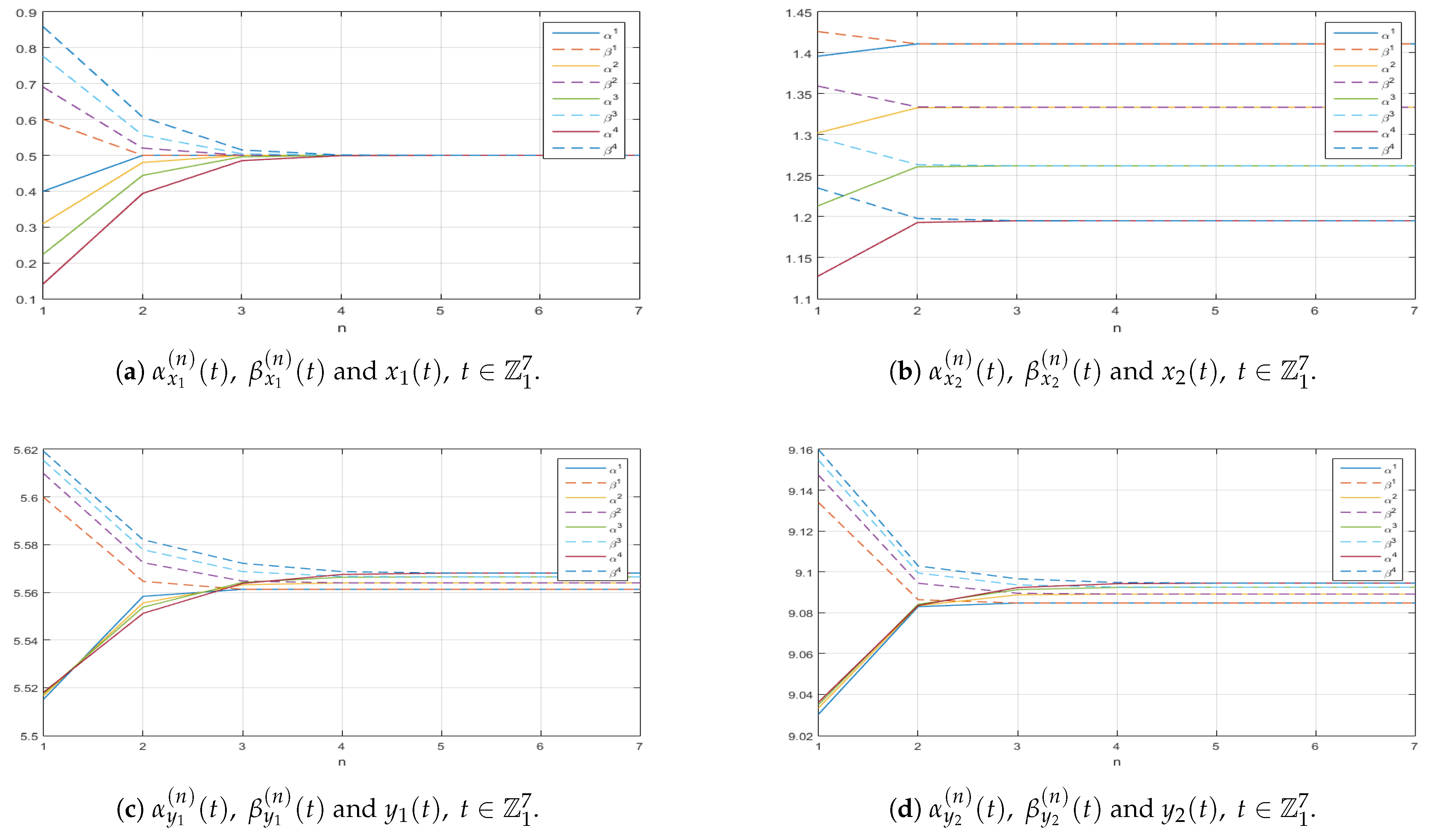
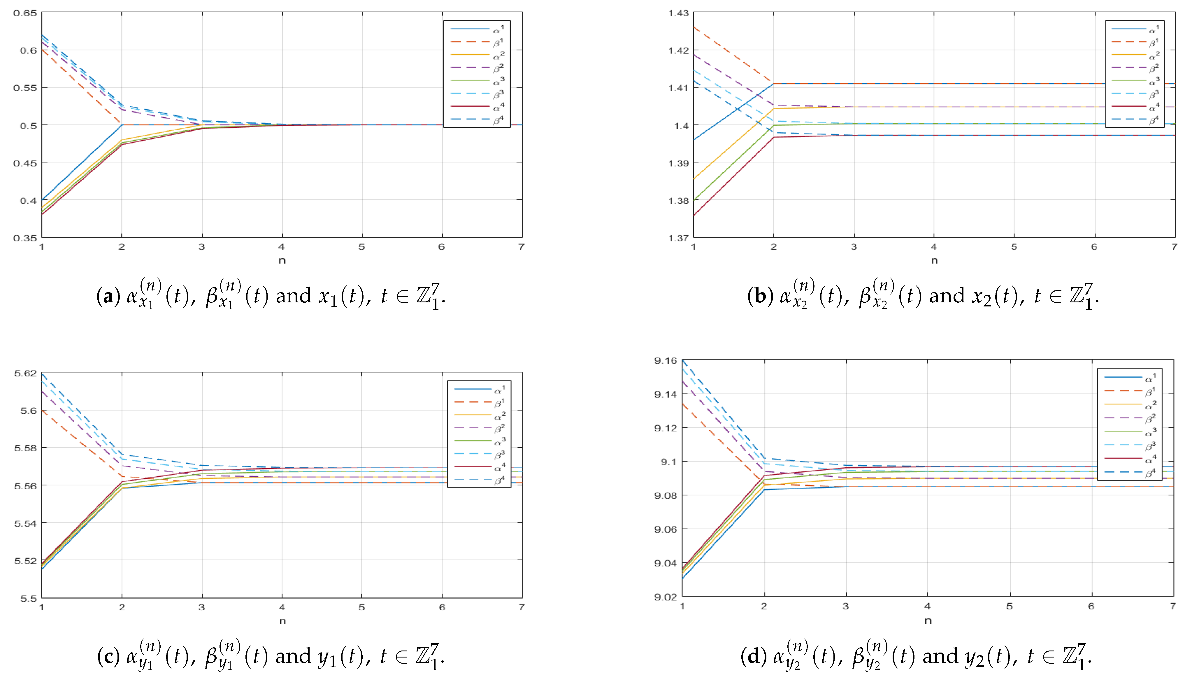
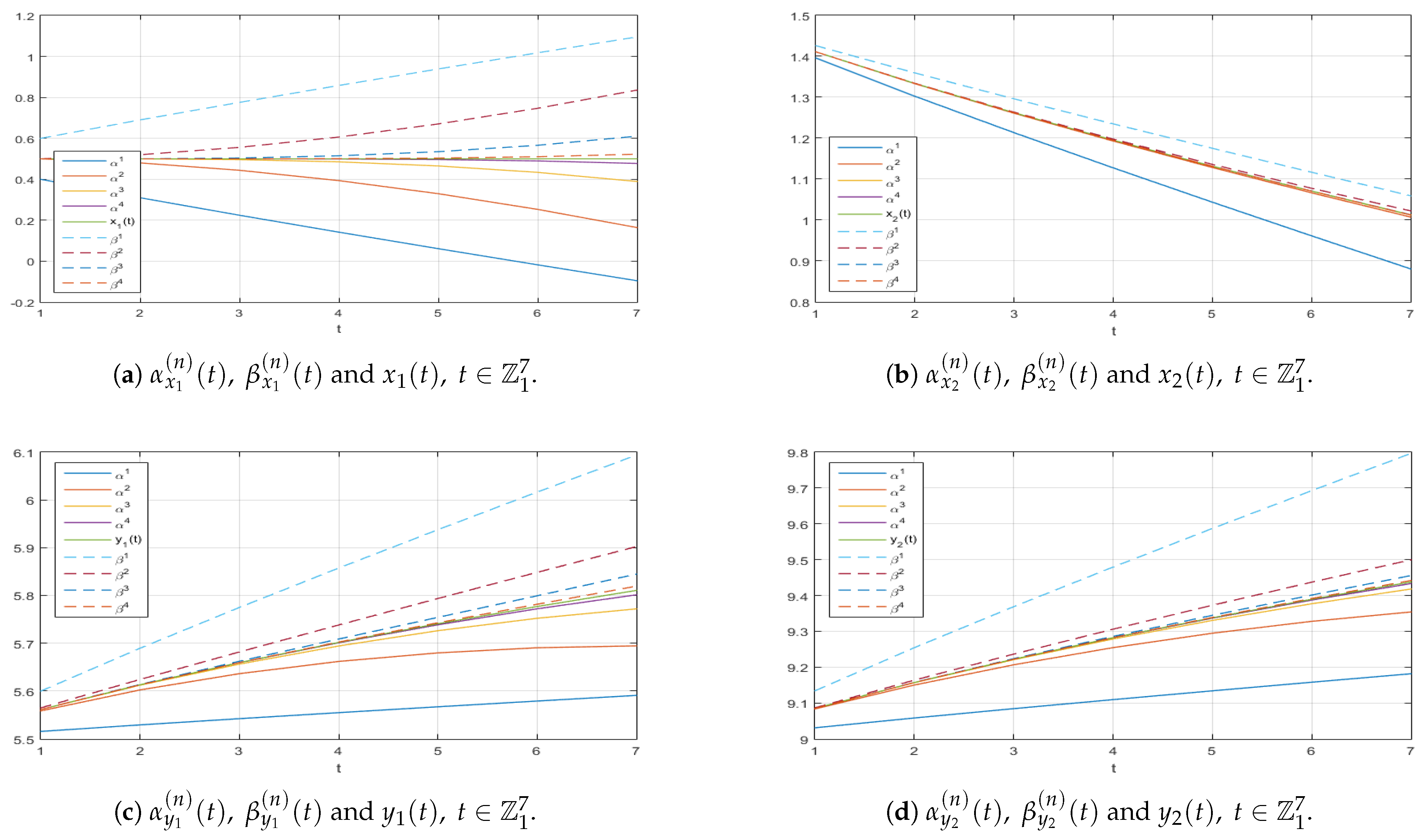
- The sequences and , representing mild lower and upper solutions, respectively, demonstrate distinct monotonic behaviors. Specifically, the sequence is non-decreasing while the sequence is non-increasing. This behavior is clearly illustrated in Figure 1, Figure 2 and Figure 3. Further supporting evidence is presented in Figure A1, Figure A2, Figure A3, Figure A4, Figure A5, Figure A6 and Figure A7 within the Appendix B. Additionally, Table 1 and Table 2, as well as all tables included in Appendix A, provide data that reinforce these findings.
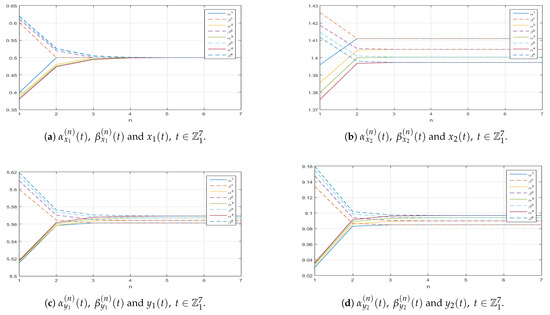 Figure 1. Graphs along the -axis of the successive approximations and to the corresponding exact solution of (11).
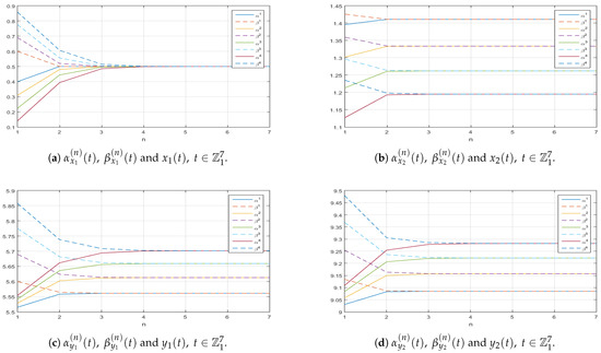 Figure 2. Graphs along the -axis of the successive approximations and , to the corresponding exact solution of (11).
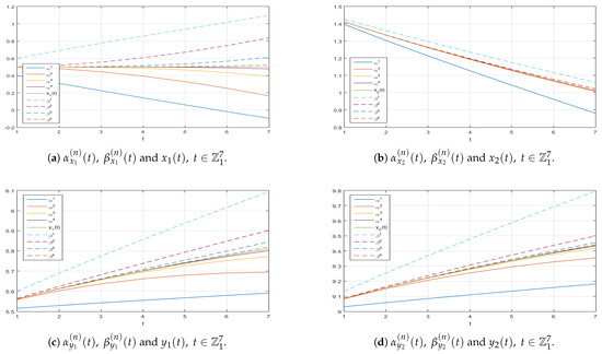 Figure 3. Graphs along the -axis of the successive approximations and to the corresponding exact solution of (11).
 Table 1. Values of the mild lower solutions and the exact solution of (11) for .
Table 2. Values of the mild lower solutions and the exact solution of (11) for .
Table 1. Values of the mild lower solutions and the exact solution of (11) for .
Table 2. Values of the mild lower solutions and the exact solution of (11) for . - -
- -
- -
- Smaller fractional orders (refer to specific Figure 1 and Figure A1, and Table 1 and Table A9, Table A10, Table A11, Table A12, Table A13, Table A14 and Table A15) enhance the convergence rates for variables and , with acceleration becoming more evident as the fractional order approaches zero. Conversely, larger orders, depicted in certain Figure 2 and Figure 3 and Table 2 and Table A16, Table A17, Table A18, Table A19, Table A20, Table A21 and Table A22 nearing one, tend to decelerate this process.
To provide clarity on these findings, Appendix A provides tables detailing absolute errors between mild solutions derived through approximations across various fractional orders. Furthermore, concerning temporal accuracy (as demonstrated in Appendix A and Appendix B), any observed decrease in convergence over time is not an inherent limitation but rather contingent upon the discretization choices, which can be adjusted according to the specific application requirements.
In conclusion, the presented graphs and tables effectively demonstrate the collective influence of iteration dynamics, time factors, and fractional order variations on convergence rates and accuracy levels.
5. Final Comments and Conclusions
This study examines nonlinear fractional difference equations with constant delay, using the Caputo-type nabla operator in discrete time over a compact interval. The order of the fractional difference operator affects interval discretization and summation representation, as discussed in [17,40]. Integer discretization is assumed for this analysis. Despite advances in continuous operators, discrete models remain essential due to progress in informatics. We have established sufficient conditions ensuring uniform convergence of two monotonous sequences of functions (specifically ), allowing for the approximation of extremal solutions through equivalent summation representations. These theoretical results have been applied to a discrete model of BAM neural networks.
Future research could explore specific models in science, engineering, or neurocomputing to further elucidate applications. By analyzing various types of fractional operators and examining scenarios where mild lower and upper solutions exist at varying initial times (see [31]), researchers can devise iterative schemes to obtain extremal mild solutions for initial value problems. Another direction involves incorporating spatial operators, as demonstrated in the study [41] on a nonlinear fractional Schrödinger–Poisson system:
where is the fractional Laplacian of order and is a potential function.
Similarly, ref. [42] discusses existence results for discrete fractional boundary value problems under nonlinear growth conditions through Schaefer’s fixed point theorem. In work [43], positive solutions for discrete delta-nabla boundary value problems with p-Laplacian operators () can be approximated using techniques such as upper and lower solution methods combined with Schauder’s fixed point theorem. For continuous cases, sufficient conditions for the existence and uniqueness of positive solutions are presented in [44,45].
Author Contributions
Conceptualization, R.P.A. and E.M.; Formal analysis, R.P.A. and E.M.; Writing—review & editing, R.P.A. and E.M.; Visualization, E.M.; Supervision, R.P.A. The authors contribution in the article are equal. All authors have read and agreed to the published version of the manuscript.
Funding
The paper has been supported by Bulgarian National Science Fund, Grant KP-06-N52/4.
Data Availability Statement
The datasets produced in this study can be requested from the authors.
Acknowledgments
The authors are thankful to anonymous reviewers for their very helpful comments and suggestions.
Conflicts of Interest
The authors declare no conflict of interest.
Abbreviations
The following abbreviations are used in this manuscript:
| Caputo-type Fractional Nabla Difference Equation | |
| Initial Value Problem | |
| Caputo-type Fractional Nabla Difference System | |
| Coupled of mild lower and upper solutions | |
| Absolute error | |
| BAM | Bidirectional associative memory |
Appendix A. Tables of the Numerical Simulations of Example 1
Table A1.
Values of the mild lower solutions and the exact solution of (11) for .
Table A1.
Values of the mild lower solutions and the exact solution of (11) for .
| t | ||||||||
|---|---|---|---|---|---|---|---|---|
| 1 | 0.437996368 | 0.537998704 | 0.537998814 | 0.537998821 | 0.537998821 | 0.537998821 | 0.537998821 | 1.11022 |
| 2 | 0.406994552 | 0.529398185 | 0.549398534 | 0.54939857 | 0.549398573 | 0.549398573 | 0.549398573 | 2.22045 |
| 3 | 0.38374319 | 0.516047841 | 0.553568246 | 0.557568418 | 0.557568433 | 0.557568434 | 0.557568434 | 1.88738 |
| 4 | 0.364367055 | 0.500322584 | 0.554122943 | 0.563019312 | 0.563819353 | 0.563819356 | 0.563819357 | 2.47345 |
| 5 | 0.347412937 | 0.483113009 | 0.552263237 | 0.566451852 | 0.568752724 | 0.568912737 | 0.568912738 | 1.26572 |
| 6 | 0.332154231 | 0.464864411 | 0.548589437 | 0.568216337 | 0.572669243 | 0.573185114 | 0.573217118 | 3.20039 |
| 7 | 0.318167084 | 0.445836546 | 0.543458181 | 0.568513153 | 0.57573209 | 0.576815512 | 0.576945952 | 0.000130441 |
Table A2.
Values of the mild upper solutions and the exact solution of (11) for .
Table A2.
Values of the mild upper solutions and the exact solution of (11) for .
| t | ||||||||
|---|---|---|---|---|---|---|---|---|
| 1 | 0.637999509 | 0.537998906 | 0.537998828 | 0.537998821 | 0.537998821 | 0.537998821 | 0.537998821 | 1.11022 |
| 2 | 0.706999263 | 0.569399246 | 0.54939862 | 0.549398576 | 0.549398573 | 0.549398573 | 0.549398573 | 2.88658 |
| 3 | 0.758749079 | 0.596049768 | 0.56156857 | 0.557568448 | 0.557568435 | 0.557568434 | 0.557568434 | 6.77236 |
| 4 | 0.801873926 | 0.620325376 | 0.574123598 | 0.564619409 | 0.563819361 | 0.563819357 | 0.563819357 | 2.36732 |
| 5 | 0.839608166 | 0.643116661 | 0.587264296 | 0.571252061 | 0.569072752 | 0.568912739 | 0.568912738 | 1.14588 |
| 6 | 0.873568983 | 0.664868916 | 0.601090958 | 0.577816704 | 0.573789307 | 0.573249122 | 0.573217118 | 3.2004 |
| 7 | 0.904699732 | 0.685841895 | 0.615647717 | 0.584513722 | 0.57825221 | 0.57707153 | 0.576945952 | 0.000125578 |
Table A3.
Values of the mild lower solutions and the exact solution of (11) for .
Table A3.
Values of the mild lower solutions and the exact solution of (11) for .
| t | ||||||||
|---|---|---|---|---|---|---|---|---|
| 1 | 1.396000036 | 1.411000108 | 1.411000116 | 1.411000116 | 1.411000116 | 1.411000116 | 1.410999999 | 1.1783 |
| 2 | 1.344000053 | 1.368720135 | 1.369170158 | 1.369170161 | 1.369170161 | 1.369170161 | 1.369169998 | 1.62648 |
| 3 | 1.305000067 | 1.337565144 | 1.338371582 | 1.338385087 | 1.338385088 | 1.338385088 | 1.338384898 | 1.90134 |
| 4 | 1.272500078 | 1.311972644 | 1.313088697 | 1.313124453 | 1.31312486 | 1.31312486 | 1.313124651 | 2.09129 |
| 5 | 1.244062588 | 1.289856702 | 1.291247269 | 1.291312337 | 1.29131347 | 1.291313482 | 1.291313259 | 2.23015 |
| 6 | 1.218468847 | 1.270174351 | 1.271810181 | 1.271910778 | 1.271912916 | 1.271912961 | 1.271912728 | 2.33124 |
| 7 | 1.195007917 | 1.252317192 | 1.254172692 | 1.254314507 | 1.254317898 | 1.254318001 | 1.254317761 | 2.40139 |
Table A4.
Values of the mild upper solutions and the exact solution of (11) for .
Table A4.
Values of the mild upper solutions and the exact solution of (11) for .
| t | ||||||||
|---|---|---|---|---|---|---|---|---|
| 1 | 1.426000363 | 1.411000128 | 1.411000117 | 1.411000116 | 1.411000116 | 1.411000116 | 1.410999999 | 1.1783 |
| 2 | 1.389000544 | 1.369620188 | 1.369170163 | 1.369170161 | 1.369170161 | 1.369170161 | 1.369169998 | 1.62648 |
| 3 | 1.361250681 | 1.339365231 | 1.338398593 | 1.338385089 | 1.338385088 | 1.338385088 | 1.338384898 | 1.90134 |
| 4 | 1.338125794 | 1.314672766 | 1.313156216 | 1.313125266 | 1.31312486 | 1.31312486 | 1.313124651 | 2.09143 |
| 5 | 1.317891518 | 1.293456857 | 1.291365422 | 1.291314772 | 1.291313495 | 1.291313482 | 1.291313259 | 2.23073 |
| 6 | 1.29968067 | 1.274674538 | 1.271987406 | 1.271915645 | 1.271913002 | 1.271912962 | 1.271912728 | 2.34001 |
| 7 | 1.282987392 | 1.257717411 | 1.254416373 | 1.254322618 | 1.254318091 | 1.254318005 | 1.254317761 | 2.43355 |
Table A5.
Values of the mild lower solutions and the exact solution of (11) for .
Table A5.
Values of the mild lower solutions and the exact solution of (11) for .
| t | ||||||||
|---|---|---|---|---|---|---|---|---|
| 1 | 5.515231883 | 5.559582255 | 5.562412989 | 5.562412992 | 5.562412993 | 5.562412993 | 5.562412992 | 4.99545 |
| 2 | 5.52741739 | 5.600804981 | 5.608613012 | 5.609382574 | 5.609382576 | 5.609382576 | 5.609382575 | 1.11709 |
| 3 | 5.538384345 | 5.633524321 | 5.647344807 | 5.649546295 | 5.64970249 | 5.649702491 | 5.649702489 | 1.762 |
| 4 | 5.548620171 | 5.660444993 | 5.680987846 | 5.685237681 | 5.685726669 | 5.685758199 | 5.685758196 | 2.32806 |
| 5 | 5.558344205 | 5.682845799 | 5.710649797 | 5.717531562 | 5.718540337 | 5.718659097 | 5.718665373 | 6.27598 |
| 6 | 5.567679278 | 5.701477698 | 5.736972338 | 5.747041769 | 5.748762811 | 5.749046283 | 5.749073344 | 2.70609 |
| 7 | 5.576703182 | 5.716837819 | 5.760375268 | 5.774162464 | 5.776790813 | 5.777336898 | 5.777408948 | 7.20504 |
Table A6.
Values of the mild upper solutions and the exact solution of (11) for .
Table A6.
Values of the mild upper solutions and the exact solution of (11) for .
| t | ||||||||
|---|---|---|---|---|---|---|---|---|
| 1 | 5.599744318 | 5.565644401 | 5.562412995 | 5.562412993 | 5.562412993 | 5.562412993 | 5.562412992 | 4.99545 |
| 2 | 5.679539772 | 5.618922475 | 5.610120113 | 5.609382578 | 5.609382576 | 5.609382576 | 5.609382575 | 1.11709 |
| 3 | 5.751355681 | 5.667291261 | 5.651848584 | 5.649859805 | 5.649702492 | 5.649702491 | 5.649702489 | 1.82742 |
| 4 | 5.818383863 | 5.712665191 | 5.689972717 | 5.686305112 | 5.685789653 | 5.685758199 | 5.685758196 | 2.70021 |
| 5 | 5.882060635 | 5.755893791 | 5.725607424 | 5.719888876 | 5.718785287 | 5.718671658 | 5.718665373 | 6.28541 |
| 6 | 5.943190337 | 5.797449301 | 5.759406727 | 5.751306411 | 5.749362847 | 5.749101374 | 5.749073344 | 2.80299 |
| 7 | 6.002282382 | 5.837629689 | 5.791805096 | 5.781025084 | 5.777972605 | 5.777485475 | 5.777408948 | 7.65272 |
Table A7.
Values of the mild lower solutions and the exact solution of (11) for .
Table A7.
Values of the mild lower solutions and the exact solution of (11) for .
| t | ||||||||
|---|---|---|---|---|---|---|---|---|
| 1 | 9.030463766 | 9.083619004 | 9.085337684 | 9.085337686 | 9.085337686 | 9.085337686 | 9.085337685 | 9.99089 |
| 2 | 9.054834779 | 9.144167027 | 9.149628394 | 9.149998144 | 9.149998145 | 9.149998145 | 9.149998143 | 2.24417 |
| 3 | 9.076768691 | 9.194229315 | 9.204634101 | 9.205725829 | 9.205800379 | 9.20580038 | 9.205800376 | 3.60171 |
| 4 | 9.097240342 | 9.237266338 | 9.253555835 | 9.255709587 | 9.255942812 | 9.255957619 | 9.255957614 | 4.98034 |
| 5 | 9.11668841 | 9.274899763 | 9.297877978 | 9.301423768 | 9.301905311 | 9.301960772 | 9.301963711 | 2.93908 |
| 6 | 9.135358556 | 9.308073633 | 9.338457109 | 9.343715296 | 9.344538451 | 9.344670204 | 9.344682822 | 1.26173 |
| 7 | 9.153406363 | 9.337407956 | 9.375851711 | 9.383132769 | 9.384393458 | 9.384646227 | 9.384679663 | 3.3436 |
Table A8.
Values of the mild upper solutions and the exact solution of (11) for .
Table A8.
Values of the mild upper solutions and the exact solution of (11) for .
| t | ||||||||
|---|---|---|---|---|---|---|---|---|
| 1 | 9.133792986 | 9.086904479 | 9.085337687 | 9.085337686 | 9.085337686 | 9.085337686 | 9.085337685 | 9.99089 |
| 2 | 9.240827375 | 9.155798899 | 9.150367973 | 9.149998146 | 9.149998145 | 9.149998145 | 9.149998143 | 2.24417 |
| 3 | 9.337158326 | 9.21727219 | 9.206900154 | 9.205874685 | 9.20580038 | 9.20580038 | 9.205800376 | 3.63395 |
| 4 | 9.427067212 | 9.274142376 | 9.258156405 | 9.25621554 | 9.255972427 | 9.255957619 | 9.255957614 | 5.16182 |
| 5 | 9.512480655 | 9.32768352 | 9.305641728 | 9.302539911 | 9.302019856 | 9.301966663 | 9.301963711 | 2.95179 |
| 6 | 9.59447756 | 9.378613628 | 9.350232702 | 9.345733177 | 9.344817726 | 9.344695897 | 9.344682822 | 1.3075 |
| 7 | 9.673741234 | 9.427390655 | 9.392507044 | 9.386378698 | 9.384941232 | 9.384715174 | 9.384679663 | 3.55108 |
Table A9.
Values of the mild upper solutions and the exact solution of (11) for .
Table A9.
Values of the mild upper solutions and the exact solution of (11) for .
| t | ||||||||
|---|---|---|---|---|---|---|---|---|
| 1 | 0.637999509 | 0.537998906 | 0.537998828 | 0.537998821 | 0.537998821 | 0.537998821 | 0.537998821 | 1.11022 |
| 2 | 0.65179946 | 0.554199544 | 0.534198984 | 0.534198949 | 0.534198946 | 0.534198946 | 0.534198946 | 1.55431 |
| 3 | 0.659389433 | 0.558769643 | 0.540288961 | 0.536288896 | 0.536288888 | 0.536288887 | 0.536288887 | 2.9976 |
| 4 | 0.664702414 | 0.561720699 | 0.542495948 | 0.537791901 | 0.536991873 | 0.53699187 | 0.53699187 | 2.72584 |
| 5 | 0.668819974 | 0.563945763 | 0.544037363 | 0.53875172 | 0.537852482 | 0.537692477 | 0.537692477 | 6.06242 |
| 6 | 0.672196374 | 0.565748491 | 0.545257291 | 0.53951253 | 0.538499685 | 0.538279521 | 0.538247519 | 3.20016 |
| 7 | 0.675066313 | 0.56727208 | 0.546278949 | 0.540151944 | 0.539042693 | 0.538774433 | 0.538725663 | 4.87704 |
Table A10.
Values of the mild lower solutions and the exact solution of (11) for .
Table A10.
Values of the mild lower solutions and the exact solution of (11) for .
| t | ||||||||
|---|---|---|---|---|---|---|---|---|
| 1 | 1.396000036 | 1.411000108 | 1.411000116 | 1.411000116 | 1.411000116 | 1.411000116 | 1.410999999 | 1.1783 |
| 2 | 1.385600039 | 1.404320105 | 1.404770122 | 1.404770124 | 1.404770124 | 1.404770124 | 1.404769998 | 1.25378 |
| 3 | 1.379880041 | 1.399869108 | 1.400315527 | 1.400329029 | 1.400329029 | 1.400329029 | 1.400328898 | 1.30508 |
| 4 | 1.375876043 | 1.39670901 | 1.39718135 | 1.3972009 | 1.397201305 | 1.397201305 | 1.397201171 | 1.34075 |
| 5 | 1.372772944 | 1.394248834 | 1.394742523 | 1.394765505 | 1.394765988 | 1.394766 | 1.394765863 | 1.36826 |
| 6 | 1.370228402 | 1.392227582 | 1.392738959 | 1.392764519 | 1.392765073 | 1.392765093 | 1.392764955 | 1.38704 |
| 7 | 1.368065543 | 1.390507955 | 1.3910344 | 1.391062072 | 1.391062686 | 1.391062712 | 1.391062571 | 1.40447 |
Table A11.
Values of the mild upper solutions and the exact solution of (11) for .
Table A11.
Values of the mild upper solutions and the exact solution of (11) for .
| t | ||||||||
|---|---|---|---|---|---|---|---|---|
| 1 | 1.426000363 | 1.411000128 | 1.411000117 | 1.411000116 | 1.411000116 | 1.411000116 | 1.410999999 | 1.1783 |
| 2 | 1.418600399 | 1.40522014 | 1.404770125 | 1.404770124 | 1.404770124 | 1.404770124 | 1.404769998 | 1.25378 |
| 3 | 1.414530419 | 1.400949146 | 1.400342531 | 1.400329029 | 1.400329029 | 1.400329029 | 1.400328898 | 1.30508 |
| 4 | 1.411681433 | 1.397897051 | 1.397216455 | 1.397201711 | 1.397201306 | 1.397201305 | 1.397201171 | 1.34093 |
| 5 | 1.409473469 | 1.395516077 | 1.394782894 | 1.39476664 | 1.394766013 | 1.394766 | 1.394765863 | 1.36854 |
| 6 | 1.407662938 | 1.393558187 | 1.392783366 | 1.392765881 | 1.39276511 | 1.392765094 | 1.392764955 | 1.3947 |
| 7 | 1.406123987 | 1.391891784 | 1.391082138 | 1.391063616 | 1.391062732 | 1.391062713 | 1.391062571 | 1.41657 |
Table A12.
Values of the mild lower solutions and the exact solution of (11) for .
Table A12.
Values of the mild lower solutions and the exact solution of (11) for .
| t | ||||||||
|---|---|---|---|---|---|---|---|---|
| 1 | 5.515231883 | 5.559582255 | 5.562412989 | 5.562412992 | 5.562412993 | 5.562412993 | 5.562412992 | 4.99545 |
| 2 | 5.516755071 | 5.559933536 | 5.564613122 | 5.565391586 | 5.565391587 | 5.565391587 | 5.565391586 | 5.62432 |
| 3 | 5.517592825 | 5.561991456 | 5.567221372 | 5.568234381 | 5.568393565 | 5.568393565 | 5.568393565 | 5.78969 |
| 4 | 5.518179253 | 5.56353138 | 5.569106674 | 5.570247933 | 5.570431954 | 5.570464276 | 5.570464275 | 5.60552 |
| 5 | 5.518633734 | 5.564747011 | 5.570584641 | 5.571828226 | 5.572036905 | 5.572081596 | 5.572088064 | 6.46791 |
| 6 | 5.519006408 | 5.565750227 | 5.571801776 | 5.57312997 | 5.573359197 | 5.573413659 | 5.573423525 | 9.86656 |
| 7 | 5.519323182 | 5.566604573 | 5.572837798 | 5.574238658 | 5.574485531 | 5.574548204 | 5.574560932 | 1.27281 |
Table A13.
Values of the mild upper solutions and the exact solution of (11) for .
Table A13.
Values of the mild upper solutions and the exact solution of (11) for .
| t | ||||||||
|---|---|---|---|---|---|---|---|---|
| 1 | 5.599744318 | 5.565644401 | 5.562412995 | 5.562412993 | 5.562412993 | 5.562412993 | 5.562412992 | 4.99545 |
| 2 | 5.60971875 | 5.571534931 | 5.566138125 | 5.565391588 | 5.565391587 | 5.565391587 | 5.565391586 | 5.62433 |
| 3 | 5.615204687 | 5.575174147 | 5.569419413 | 5.568553867 | 5.568393566 | 5.568393565 | 5.568393565 | 6.52062 |
| 4 | 5.619044843 | 5.577756131 | 5.5716654 | 5.570705679 | 5.570496523 | 5.570464276 | 5.570464275 | 7.62753 |
| 5 | 5.622020964 | 5.579769748 | 5.573411927 | 5.572379322 | 5.572134238 | 5.572094536 | 5.572088064 | 6.47217 |
| 6 | 5.624461384 | 5.581427399 | 5.574847942 | 5.573755213 | 5.573480935 | 5.573434379 | 5.573423525 | 1.08534 |
| 7 | 5.62653574 | 5.582840358 | 5.576070925 | 5.57492671 | 5.574627562 | 5.574575135 | 5.574560932 | 1.42035 |
Table A14.
Values of the mild lower solutions and the exact solution of (11) for .
Table A14.
Values of the mild lower solutions and the exact solution of (11) for .
| t | ||||||||
|---|---|---|---|---|---|---|---|---|
| 1 | 9.030463766 | 9.083619004 | 9.085337684 | 9.085337686 | 9.085337686 | 9.085337686 | 9.085337685 | 9.99089 |
| 2 | 9.033510143 | 9.086434568 | 9.089973068 | 9.090347081 | 9.090347081 | 9.090347081 | 9.09034708 | 1.13486 |
| 3 | 9.03518565 | 9.089835825 | 9.093881243 | 9.094405422 | 9.094481404 | 9.094481404 | 9.094481403 | 1.22325 |
| 4 | 9.036358505 | 9.09231546 | 9.096671916 | 9.097266809 | 9.097355401 | 9.097370586 | 9.097370585 | 1.27427 |
| 5 | 9.037267468 | 9.094259342 | 9.098850207 | 9.099500692 | 9.099601414 | 9.099622432 | 9.099625466 | 3.03425 |
| 6 | 9.038012817 | 9.095859784 | 9.10064124 | 9.10133736 | 9.101448153 | 9.101473773 | 9.101478401 | 4.62772 |
| 7 | 9.038646364 | 9.097221846 | 9.102165037 | 9.102900195 | 9.103019626 | 9.103049114 | 9.103055083 | 5.96959 |
Table A15.
Values of the mild upper solutions and the exact solution of (11) for .
Table A15.
Values of the mild upper solutions and the exact solution of (11) for .
| t | ||||||||
|---|---|---|---|---|---|---|---|---|
| 1 | 9.133792986 | 9.086904479 | 9.085337687 | 9.085337686 | 9.085337686 | 9.085337686 | 9.085337685 | 9.99089 |
| 2 | 9.147172285 | 9.094501763 | 9.090721222 | 9.090347082 | 9.090347081 | 9.090347081 | 9.09034708 | 1.13486 |
| 3 | 9.154530899 | 9.099117704 | 9.095018481 | 9.094557141 | 9.094481404 | 9.094481404 | 9.094481403 | 1.2593 |
| 4 | 9.159681929 | 9.102377415 | 9.098003904 | 9.097485646 | 9.097385772 | 9.097370586 | 9.097370585 | 1.37217 |
| 5 | 9.163673977 | 9.104912015 | 9.100325575 | 9.099764451 | 9.099647207 | 9.099628503 | 9.099625466 | 3.03658 |
| 6 | 9.166947457 | 9.10699393 | 9.102232933 | 9.101636747 | 9.10150543 | 9.101483492 | 9.101478401 | 5.09094 |
| 7 | 9.169729915 | 9.108765377 | 9.103855848 | 9.103229743 | 9.103086453 | 9.103061745 | 9.103055083 | 6.66205 |
Table A16.
Values of the mild upper solutions and the exact solution of (11) for .
Table A16.
Values of the mild upper solutions and the exact solution of (11) for .
| t | ||||||||
|---|---|---|---|---|---|---|---|---|
| 1 | 0.637999509 | 0.537998906 | 0.537998828 | 0.537998821 | 0.537998821 | 0.537998821 | 0.537998821 | 1.11022 |
| 2 | 0.762199067 | 0.584598827 | 0.564598168 | 0.564598118 | 0.564598115 | 0.564598115 | 0.564598115 | 1.77636 |
| 3 | 0.880188647 | 0.639409504 | 0.588927844 | 0.584927682 | 0.584927667 | 0.584927666 | 0.584927666 | 9.65894 |
| 4 | 0.994245241 | 0.70206583 | 0.616086779 | 0.601782453 | 0.600982388 | 0.600982383 | 0.600982382 | 2.27345 |
| 5 | 1.10545042 | 0.772270365 | 0.650021946 | 0.617523047 | 0.614063659 | 0.613903639 | 0.613903637 | 1.53252 |
| 6 | 1.214431496 | 0.849779164 | 0.694117363 | 0.634423227 | 0.625333193 | 0.624472981 | 0.624440974 | 3.20066 |
| 7 | 1.321596221 | 0.934387826 | 0.751413616 | 0.654780323 | 0.636057464 | 0.63332433 | 0.633121941 | 0.000202389 |
Table A17.
Values of the mild lower solutions and the exact solution of (11) for .
Table A17.
Values of the mild lower solutions and the exact solution of (11) for .
| t | ||||||||
|---|---|---|---|---|---|---|---|---|
| 1 | 1.396000036 | 1.411000108 | 1.411000116 | 1.411000116 | 1.411000116 | 1.411000116 | 1.410999999 | 1.1783 |
| 2 | 1.302400068 | 1.333120176 | 1.333570203 | 1.333570206 | 1.333570206 | 1.333570206 | 1.333569998 | 2.08389 |
| 3 | 1.213480098 | 1.261021218 | 1.262187671 | 1.262201179 | 1.262201179 | 1.262201179 | 1.262200897 | 2.82693 |
| 4 | 1.127524128 | 1.19305714 | 1.195104906 | 1.195156867 | 1.195157274 | 1.195157274 | 1.195156929 | 3.45128 |
| 5 | 1.043717056 | 1.128423847 | 1.131440519 | 1.131567113 | 1.131568896 | 1.131568908 | 1.13156851 | 3.98269 |
| 6 | 0.961586127 | 1.066642179 | 1.070650106 | 1.070898897 | 1.070903657 | 1.070903727 | 1.070903283 | 4.43489 |
| 7 | 0.880824046 | 1.007392475 | 1.012356153 | 1.012786378 | 1.012796358 | 1.012796589 | 1.012796108 | 4.80863 |
Table A18.
Values of the mild upper solutions and the exact solution of (11) for .
Table A18.
Values of the mild upper solutions and the exact solution of (11) for .
| t | ||||||||
|---|---|---|---|---|---|---|---|---|
| 1 | 1.426000363 | 1.411000128 | 1.411000117 | 1.411000116 | 1.411000116 | 1.411000116 | 1.410999999 | 1.1783 |
| 2 | 1.35940069 | 1.334020239 | 1.333570209 | 1.333570206 | 1.333570206 | 1.333570206 | 1.333569998 | 2.08389 |
| 3 | 1.296131 | 1.263541341 | 1.262214687 | 1.26220118 | 1.262201179 | 1.262201179 | 1.262200897 | 2.82693 |
| 4 | 1.2349703 | 1.197845336 | 1.195204837 | 1.195157681 | 1.195157274 | 1.195157274 | 1.195156929 | 3.45141 |
| 5 | 1.175338617 | 1.136084928 | 1.131675336 | 1.131570848 | 1.131568921 | 1.131568909 | 1.13156851 | 3.98345 |
| 6 | 1.116899568 | 1.077750714 | 1.071096239 | 1.070909347 | 1.070903793 | 1.070903728 | 1.070903283 | 4.4448 |
| 7 | 1.059434504 | 1.02250005 | 1.013103405 | 1.012809357 | 1.012796797 | 1.012796594 | 1.012796108 | 4.86216 |
Table A19.
Values of the mild lower solutions and the exact solution of (11) for .
Table A19.
Values of the mild lower solutions and the exact solution of (11) for .
| t | ||||||||
|---|---|---|---|---|---|---|---|---|
| 1 | 5.515231883 | 5.559582255 | 5.562412989 | 5.562412992 | 5.562412993 | 5.562412993 | 5.562412992 | 4.99545 |
| 2 | 5.528940578 | 5.605910915 | 5.615148081 | 5.615908669 | 5.615908671 | 5.615908671 | 5.615908669 | 1.43694 |
| 3 | 5.541963838 | 5.64348346 | 5.661463116 | 5.664261419 | 5.66441386 | 5.66441386 | 5.664413858 | 2.76659 |
| 4 | 5.554552989 | 5.673738515 | 5.701981981 | 5.70846327 | 5.709120406 | 5.709150845 | 5.709150841 | 4.36036 |
| 5 | 5.566827412 | 5.697390786 | 5.736718761 | 5.748842684 | 5.750567755 | 5.750729859 | 5.750735857 | 5.9987 |
| 6 | 5.578856346 | 5.714865941 | 5.76542356 | 5.785442927 | 5.789004977 | 5.789516275 | 5.789553885 | 3.76107 |
| 7 | 5.590684798 | 5.726444089 | 5.787696489 | 5.818135839 | 5.824496575 | 5.825740395 | 5.82587696 | 0.000136565 |
Table A20.
Values of the mild upper solutions and the exact solution of (11) for .
Table A20.
Values of the mild upper solutions and the exact solution of (11) for .
| t | ||||||||
|---|---|---|---|---|---|---|---|---|
| 1 | 5.599744318 | 5.565644401 | 5.562412995 | 5.562412993 | 5.562412993 | 5.562412993 | 5.562412992 | 4.99545 |
| 2 | 5.689514204 | 5.626830065 | 5.616637149 | 5.615908673 | 5.615908671 | 5.615908671 | 5.615908669 | 1.43694 |
| 3 | 5.774795596 | 5.68643966 | 5.667107117 | 5.664567419 | 5.664413861 | 5.66441386 | 5.664413858 | 2.82886 |
| 4 | 5.857234274 | 5.745069132 | 5.715387739 | 5.70986285 | 5.709181209 | 5.709150846 | 5.709150841 | 4.8081 |
| 5 | 5.937611986 | 5.802863926 | 5.762338764 | 5.752735373 | 5.750898861 | 5.750741872 | 5.750735857 | 6.01522 |
| 6 | 6.016382144 | 5.85983143 | 5.808516071 | 5.793946651 | 5.790071776 | 5.789592423 | 5.789553885 | 3.85376 |
| 7 | 6.093839465 | 5.915932078 | 5.854306341 | 5.834174288 | 5.827143799 | 5.826019805 | 5.82587696 | 0.000142845 |
Table A21.
Values of the mild lower solutions and the exact solution of (11) for .
Table A21.
Values of the mild lower solutions and the exact solution of (11) for .
| t | ||||||||
|---|---|---|---|---|---|---|---|---|
| 1 | 9.030463766 | 9.083619004 | 9.085337684 | 9.085337686 | 9.085337686 | 9.085337686 | 9.085337685 | 9.99089 |
| 2 | 9.057881156 | 9.151691185 | 9.158057338 | 9.158422799 | 9.1584228 | 9.1584228 | 9.158422797 | 2.88387 |
| 3 | 9.083927676 | 9.209981145 | 9.223217821 | 9.224602611 | 9.224675351 | 9.224675351 | 9.224675345 | 5.61593 |
| 4 | 9.109105979 | 9.260271505 | 9.282207933 | 9.285470794 | 9.28578544 | 9.285799724 | 9.285799715 | 9.12941 |
| 5 | 9.133654824 | 9.303409651 | 9.335568757 | 9.341743073 | 9.342572056 | 9.342648157 | 9.342650958 | 2.80144 |
| 6 | 9.157712692 | 9.339870573 | 9.383498084 | 9.393778588 | 9.395497158 | 9.395737306 | 9.395754921 | 1.76152 |
| 7 | 9.181369596 | 9.36994133 | 9.426014801 | 9.441744015 | 9.444826529 | 9.445411118 | 9.445475115 | 6.39974 |
Table A22.
Values of the mild upper solutions and the exact solution of (11) for .
Table A22.
Values of the mild upper solutions and the exact solution of (11) for .
| t | ||||||||
|---|---|---|---|---|---|---|---|---|
| 1 | 9.133792986 | 9.086904479 | 9.085337687 | 9.085337686 | 9.085337686 | 9.085337686 | 9.085337685 | 9.99089 |
| 2 | 9.254206674 | 9.164893049 | 9.158788296 | 9.158422801 | 9.1584228 | 9.1584228 | 9.158422797 | 2.88387 |
| 3 | 9.368599677 | 9.238558428 | 9.226053461 | 9.224747845 | 9.224675351 | 9.224675351 | 9.224675345 | 5.64667 |
| 4 | 9.479179581 | 9.309143523 | 9.289035811 | 9.286136842 | 9.285814009 | 9.285799725 | 9.285799715 | 9.34908 |
| 5 | 9.586994986 | 9.377161615 | 9.348741636 | 9.343599077 | 9.34272765 | 9.342653787 | 9.342650958 | 2.82843 |
| 6 | 9.692654084 | 9.442861651 | 9.405815033 | 9.397838947 | 9.395998552 | 9.395772988 | 9.395754921 | 1.80672 |
| 7 | 9.796552196 | 9.506372671 | 9.460713338 | 9.449410796 | 9.446070964 | 9.445542045 | 9.445475115 | 6.69295 |
Table A23.
Values of the mild lower solutions and the exact solution of (11) for .
Table A23.
Values of the mild lower solutions and the exact solution of (11) for .
| t | ||||||||
|---|---|---|---|---|---|---|---|---|
| 1 | 0.437996368 | 0.537998704 | 0.537998814 | 0.537998821 | 0.537998821 | 0.537998821 | 0.537998821 | 1.11022 |
| 2 | 0.431796005 | 0.514198708 | 0.534199023 | 0.534199054 | 0.534199057 | 0.534199057 | 0.534199057 | 1.44329 |
| 3 | 0.428385805 | 0.510768692 | 0.532288916 | 0.536289065 | 0.536289076 | 0.536289077 | 0.536289077 | 1.11022 |
| 4 | 0.425998665 | 0.50891969 | 0.532095901 | 0.536192105 | 0.536992131 | 0.536992133 | 0.536992133 | 2.45781 |
| 5 | 0.424148632 | 0.50762472 | 0.53207732 | 0.536511967 | 0.537532797 | 0.537692805 | 0.537692806 | 8.27044 |
| 6 | 0.422631605 | 0.506611426 | 0.532101252 | 0.536824817 | 0.538020052 | 0.538215905 | 0.538247907 | 3.20018 |
| 7 | 0.421342131 | 0.505769561 | 0.532136212 | 0.537105866 | 0.538443107 | 0.538672468 | 0.538726103 | 5.36347 |
Table A24.
Values of the mild upper solutions and the exact solution of (11) for .
Table A24.
Values of the mild upper solutions and the exact solution of (11) for .
| t | ||||||||
|---|---|---|---|---|---|---|---|---|
| 1 | 0.637999509 | 0.537998906 | 0.537998828 | 0.537998821 | 0.537998821 | 0.537998821 | 0.537998821 | 1.11022 |
| 2 | 0.65179946 | 0.554199702 | 0.5341991 | 0.53419906 | 0.534199057 | 0.534199057 | 0.534199057 | 2.10942 |
| 3 | 0.659389433 | 0.558769949 | 0.540289182 | 0.536289088 | 0.536289078 | 0.536289077 | 0.536289077 | 4.10783 |
| 4 | 0.664702414 | 0.561721135 | 0.542496265 | 0.537792172 | 0.536992137 | 0.536992134 | 0.536992133 | 2.35219 |
| 5 | 0.668819974 | 0.563946315 | 0.544037768 | 0.538752064 | 0.537852813 | 0.537692806 | 0.537692806 | 7.24212 |
| 6 | 0.672196374 | 0.565749144 | 0.545257775 | 0.539512942 | 0.538500077 | 0.538279909 | 0.538247907 | 3.20021 |
| 7 | 0.675066313 | 0.567272822 | 0.546279505 | 0.540152418 | 0.53904314 | 0.538774874 | 0.538726103 | 4.87715 |
Table A25.
Values of the mild lower solutions and the exact solution of (11) for .
Table A25.
Values of the mild lower solutions and the exact solution of (11) for .
| t | ||||||||
|---|---|---|---|---|---|---|---|---|
| 1 | 1.396000036 | 1.411000108 | 1.411000116 | 1.411000116 | 1.411000116 | 1.411000116 | 1.410999999 | 1.1783 |
| 2 | 1.385600039 | 1.40432009 | 1.404770111 | 1.404770113 | 1.404770113 | 1.404770113 | 1.404769999 | 1.1425 |
| 3 | 1.379880041 | 1.399869077 | 1.400315504 | 1.400329008 | 1.400329008 | 1.400329008 | 1.400328899 | 1.09636 |
| 4 | 1.375876043 | 1.396708966 | 1.397181317 | 1.397200871 | 1.397201276 | 1.397201276 | 1.397201172 | 1.04378 |
| 5 | 1.372772944 | 1.394248779 | 1.394742481 | 1.394765467 | 1.394765951 | 1.394765963 | 1.394765864 | 9.91774 |
| 6 | 1.370228402 | 1.392227517 | 1.392738909 | 1.392764474 | 1.392765029 | 1.392765049 | 1.392764955 | 9.38812 |
| 7 | 1.368065543 | 1.390507882 | 1.391034342 | 1.391062021 | 1.391062635 | 1.391062661 | 1.391062572 | 8.91302 |
Table A26.
Values of the mild upper solutions and the exact solution of (11) for .
Table A26.
Values of the mild upper solutions and the exact solution of (11) for .
| t | ||||||||
|---|---|---|---|---|---|---|---|---|
| 1 | 1.426000363 | 1.411000128 | 1.411000117 | 1.411000116 | 1.411000116 | 1.411000116 | 1.410999999 | 1.1783 |
| 2 | 1.418600399 | 1.405220137 | 1.404770115 | 1.404770113 | 1.404770113 | 1.404770113 | 1.404769999 | 1.1425 |
| 3 | 1.414530419 | 1.40094914 | 1.400342512 | 1.400329009 | 1.400329008 | 1.400329008 | 1.400328899 | 1.09636 |
| 4 | 1.411681433 | 1.397897042 | 1.397216429 | 1.397201682 | 1.397201276 | 1.397201276 | 1.397201172 | 1.04391 |
| 5 | 1.409473469 | 1.395516065 | 1.394782861 | 1.394766603 | 1.394765976 | 1.394765963 | 1.394765864 | 9.9211 |
| 6 | 1.407662938 | 1.393558172 | 1.392783329 | 1.392765838 | 1.392765066 | 1.39276505 | 1.392764955 | 9.46691 |
| 7 | 1.406123987 | 1.391891766 | 1.391082095 | 1.391063567 | 1.391062681 | 1.391062662 | 1.391062572 | 9.03859 |
Table A27.
Values of the mild lower solutions and the exact solution of (11) for .
Table A27.
Values of the mild lower solutions and the exact solution of (11) for .
| t | ||||||||
|---|---|---|---|---|---|---|---|---|
| 1 | 5.515231883 | 5.559582255 | 5.562412989 | 5.562412992 | 5.562412993 | 5.562412993 | 5.562412992 | 4.99545 |
| 2 | 5.528940578 | 5.60759934 | 5.614543514 | 5.615321983 | 5.615321984 | 5.615321984 | 5.615321983 | 9.14365 |
| 3 | 5.541963838 | 5.648847736 | 5.661223448 | 5.662988492 | 5.663147678 | 5.663147678 | 5.663147677 | 1.24112 |
| 4 | 5.554552989 | 5.684745625 | 5.703789423 | 5.706838827 | 5.707185721 | 5.707218044 | 5.707218042 | 1.44531 |
| 5 | 5.566827412 | 5.716016293 | 5.74291456 | 5.747582078 | 5.748169019 | 5.748247861 | 5.748254328 | 6.46695 |
| 6 | 5.578856346 | 5.743107942 | 5.779014354 | 5.785659546 | 5.786550797 | 5.786692348 | 5.786709085 | 1.67375 |
| 7 | 5.590684798 | 5.766330332 | 5.812376205 | 5.821376457 | 5.822649802 | 5.822872754 | 5.822903965 | 3.1211 |
Table A28.
Values of the mild upper solutions and the exact solution of (11) for .
Table A28.
Values of the mild upper solutions and the exact solution of (11) for .
| t | ||||||||
|---|---|---|---|---|---|---|---|---|
| 1 | 5.599744318 | 5.565644401 | 5.562412995 | 5.562412993 | 5.562412993 | 5.562412993 | 5.562412992 | 4.99545 |
| 2 | 5.689514204 | 5.624050452 | 5.616068526 | 5.615321986 | 5.615321984 | 5.615321984 | 5.615321983 | 9.14365 |
| 3 | 5.774795596 | 5.679056785 | 5.664883993 | 5.663307983 | 5.663147679 | 5.663147678 | 5.663147677 | 1.30766 |
| 4 | 5.857234274 | 5.731746737 | 5.710274163 | 5.707625295 | 5.707250292 | 5.707218044 | 5.707218042 | 1.74551 |
| 5 | 5.937611986 | 5.782642585 | 5.753008582 | 5.748991526 | 5.748334445 | 5.748260802 | 5.748254328 | 6.4736 |
| 6 | 6.016382144 | 5.8320517 | 5.79359873 | 5.787872485 | 5.786854604 | 5.786726825 | 5.786709085 | 1.77399 |
| 7 | 6.093839465 | 5.88017673 | 5.832424981 | 5.82460527 | 5.823134762 | 5.822937747 | 5.822903965 | 3.37821 |
Table A29.
Values of the mild lower solutions and the exact solution of (11) for .
Table A29.
Values of the mild lower solutions and the exact solution of (11) for .
| t | ||||||||
|---|---|---|---|---|---|---|---|---|
| 1 | 9.030463766 | 9.083619004 | 9.085337684 | 9.085337686 | 9.085337686 | 9.085337686 | 9.085337685 | 9.99089 |
| 2 | 9.057881156 | 9.153329771 | 9.158243215 | 9.158617231 | 9.158617231 | 9.158617231 | 9.15861723 | 1.83872 |
| 3 | 9.083927676 | 9.214907787 | 9.224521888 | 9.225395418 | 9.2254714 | 9.225471401 | 9.225471398 | 2.55775 |
| 4 | 9.109105979 | 9.270192991 | 9.285913685 | 9.287476478 | 9.287640029 | 9.287655215 | 9.287655211 | 3.15173 |
| 5 | 9.133654824 | 9.320112947 | 9.343290562 | 9.345764838 | 9.346040327 | 9.346076476 | 9.346079508 | 3.03194 |
| 6 | 9.157712692 | 9.365236504 | 9.397187134 | 9.400819533 | 9.401238667 | 9.401302149 | 9.401309808 | 7.65943 |
| 7 | 9.181369596 | 9.405953208 | 9.447970787 | 9.453026159 | 9.453629235 | 9.453727247 | 9.453741193 | 1.39457 |
Table A30.
Values of the mild upper solutions and the exact solution of (11) for .
Table A30.
Values of the mild upper solutions and the exact solution of (11) for .
| t | ||||||||
|---|---|---|---|---|---|---|---|---|
| 1 | 9.133792986 | 9.086904479 | 9.085337687 | 9.085337686 | 9.085337686 | 9.085337686 | 9.085337685 | 9.99089 |
| 2 | 9.254206674 | 9.164025346 | 9.158991374 | 9.158617232 | 9.158617232 | 9.158617231 | 9.15861723 | 1.83872 |
| 3 | 9.368599677 | 9.236315498 | 9.226362791 | 9.22554714 | 9.225471401 | 9.225471401 | 9.225471398 | 2.59046 |
| 4 | 9.479179581 | 9.305285619 | 9.289273801 | 9.287844841 | 9.287670401 | 9.287655215 | 9.287655211 | 3.2969 |
| 5 | 9.586994986 | 9.371665597 | 9.348680756 | 9.346419369 | 9.346116399 | 9.346082547 | 9.346079508 | 3.03911 |
| 6 | 9.692654084 | 9.435885844 | 9.405198722 | 9.401843125 | 9.401375461 | 9.401317936 | 9.401309808 | 8.1274 |
| 7 | 9.796552196 | 9.498230659 | 9.459271531 | 9.454519406 | 9.453843416 | 9.453756296 | 9.453741193 | 1.51031 |
Table A31.
Values of the mild lower solutions and the exact solution of (11) for .
Table A31.
Values of the mild lower solutions and the exact solution of (11) for .
| t | ||||||||
|---|---|---|---|---|---|---|---|---|
| 1 | 0.437996368 | 0.537998704 | 0.537998814 | 0.537998821 | 0.537998821 | 0.537998821 | 0.537998821 | 1.11022 |
| 2 | 0.3821931 | 0.54459764 | 0.564597962 | 0.564598 | 0.564598004 | 0.564598004 | 0.564598004 | 3.33067 |
| 3 | 0.329179994 | 0.527406714 | 0.580927189 | 0.584927368 | 0.584927385 | 0.584927386 | 0.584927386 | 2.33147 |
| 4 | 0.277933993 | 0.489260897 | 0.586485353 | 0.600181848 | 0.600981897 | 0.600981902 | 0.600981903 | 2.74048 |
| 5 | 0.227969141 | 0.431782799 | 0.580459369 | 0.610162016 | 0.613742922 | 0.61390294 | 0.613902941 | 1.7208 |
| 6 | 0.179003586 | 0.356072509 | 0.561949206 | 0.613813575 | 0.623572158 | 0.624408051 | 0.624440057 | 3.20063 |
| 7 | 0.130854124 | 0.262947093 | 0.530032697 | 0.60944018 | 0.63033605 | 0.632913554 | 0.633120803 | 0.000207249 |
Table A32.
Values of the mild upper solutions and the exact solution of (11) for .
Table A32.
Values of the mild upper solutions and the exact solution of (11) for .
| t | ||||||||
|---|---|---|---|---|---|---|---|---|
| 1 | 0.637999509 | 0.537998906 | 0.537998828 | 0.537998821 | 0.537998821 | 0.537998821 | 0.537998821 | 1.11022 |
| 2 | 0.762199067 | 0.584598669 | 0.564598053 | 0.564598007 | 0.564598004 | 0.564598004 | 0.564598004 | 9.99201 |
| 3 | 0.880188647 | 0.639409071 | 0.588927529 | 0.584927402 | 0.584927387 | 0.584927386 | 0.584927386 | 7.77156 |
| 4 | 0.994245241 | 0.702065034 | 0.616086199 | 0.601781964 | 0.600981908 | 0.600981903 | 0.600981903 | 2.63067 |
| 5 | 1.10545042 | 0.772269138 | 0.650021053 | 0.61752232 | 0.614062961 | 0.613902943 | 0.613902941 | 1.58358 |
| 6 | 1.214431496 | 0.849777449 | 0.694116121 | 0.634422231 | 0.625332265 | 0.624472063 | 0.624440057 | 3.20062 |
| 7 | 1.321596221 | 0.934385579 | 0.751412001 | 0.654779024 | 0.636056297 | 0.63332319 | 0.633120803 | 0.000202387 |
Table A33.
Values of the mild lower solutions and the exact solution of (11) for .
Table A33.
Values of the mild lower solutions and the exact solution of (11) for .
| t | ||||||||
|---|---|---|---|---|---|---|---|---|
| 1 | 1.396000036 | 1.411000108 | 1.411000116 | 1.411000116 | 1.411000116 | 1.411000116 | 1.410999999 | 1.1783 |
| 2 | 1.302400068 | 1.333120192 | 1.333570214 | 1.333570217 | 1.333570217 | 1.333570217 | 1.333569997 | 2.19505 |
| 3 | 1.213480098 | 1.261021261 | 1.262187703 | 1.262201208 | 1.262201209 | 1.262201209 | 1.262200896 | 3.12515 |
| 4 | 1.127524128 | 1.193057219 | 1.195104965 | 1.195156921 | 1.195157327 | 1.195157328 | 1.195156928 | 3.99442 |
| 5 | 1.043717056 | 1.128423969 | 1.131440612 | 1.131567196 | 1.131568978 | 1.13156899 | 1.131568509 | 4.81555 |
| 6 | 0.961586127 | 1.06664235 | 1.070650238 | 1.070899014 | 1.070903771 | 1.07090384 | 1.070903281 | 5.5925 |
| 7 | 0.880824046 | 1.007392699 | 1.012356328 | 1.012786531 | 1.012796507 | 1.012796738 | 1.012796106 | 6.3185 |
Table A34.
Values of the mild upper solutions and the exact solution of (11) for .
Table A34.
Values of the mild upper solutions and the exact solution of (11) for .
| t | ||||||||
|---|---|---|---|---|---|---|---|---|
| 1 | 1.426000363 | 1.411000128 | 1.411000117 | 1.411000116 | 1.411000116 | 1.411000116 | 1.410999999 | 1.1783 |
| 2 | 1.35940069 | 1.334020242 | 1.33357022 | 1.333570217 | 1.333570217 | 1.333570217 | 1.333569997 | 2.19505 |
| 3 | 1.296131 | 1.263541349 | 1.262214715 | 1.262201209 | 1.262201209 | 1.262201209 | 1.262200896 | 3.12515 |
| 4 | 1.2349703 | 1.197845352 | 1.195204885 | 1.195157734 | 1.195157328 | 1.195157328 | 1.195156928 | 3.99458 |
| 5 | 1.175338617 | 1.136084954 | 1.131675407 | 1.131570929 | 1.131569003 | 1.13156899 | 1.131568509 | 4.81643 |
| 6 | 1.116899568 | 1.077750751 | 1.071096335 | 1.070909458 | 1.070903907 | 1.070903841 | 1.070903281 | 5.60257 |
| 7 | 1.059434504 | 1.022500101 | 1.013103525 | 1.012809501 | 1.012796945 | 1.012796743 | 1.012796106 | 6.37197 |
Table A35.
Values of the mild lower solutions and the exact solution of (11) for .
Table A35.
Values of the mild lower solutions and the exact solution of (11) for .
| t | ||||||||
|---|---|---|---|---|---|---|---|---|
| 1 | 5.515231883 | 5.559582255 | 5.562412989 | 5.562412992 | 5.562412993 | 5.562412993 | 5.562412992 | 4.99545 |
| 2 | 5.516755071 | 5.558245111 | 5.565217689 | 5.565978272 | 5.565978273 | 5.565978273 | 5.565978272 | 1.0913 |
| 3 | 5.517592825 | 5.557977921 | 5.566977386 | 5.569037957 | 5.569190395 | 5.569190396 | 5.569190394 | 1.76058 |
| 4 | 5.518179253 | 5.556950764 | 5.567170315 | 5.57082984 | 5.571330221 | 5.571360659 | 5.571360656 | 2.4298 |
| 5 | 5.518633734 | 5.555410363 | 5.566113823 | 5.571765513 | 5.572821677 | 5.572951442 | 5.572957443 | 6.00164 |
| 6 | 5.519006408 | 5.553490574 | 5.563897531 | 5.571960302 | 5.573790236 | 5.574133496 | 5.5741647 | 3.12043 |
| 7 | 5.519323182 | 5.551267629 | 5.560527401 | 5.571440372 | 5.574264932 | 5.574988397 | 5.575085797 | 9.74004 |
Table A36.
Values of the mild upper solutions and the exact solution of (11) for .
Table A36.
Values of the mild upper solutions and the exact solution of (11) for .
| t | ||||||||
|---|---|---|---|---|---|---|---|---|
| 1 | 5.599744318 | 5.565644401 | 5.562412995 | 5.562412993 | 5.562412993 | 5.562412993 | 5.562412992 | 4.99545 |
| 2 | 5.60971875 | 5.574314544 | 5.566706748 | 5.565978275 | 5.565978274 | 5.565978273 | 5.565978272 | 1.0913 |
| 3 | 5.615204687 | 5.580333331 | 5.571187636 | 5.569343952 | 5.569190397 | 5.569190396 | 5.569190394 | 1.82891 |
| 4 | 5.619044843 | 5.584949856 | 5.574887442 | 5.571912927 | 5.571391022 | 5.571360659 | 5.571360656 | 2.81024 |
| 5 | 5.622020964 | 5.588653596 | 5.578227111 | 5.574222447 | 5.573088315 | 5.572963455 | 5.572957443 | 6.01168 |
| 6 | 5.624461384 | 5.591679092 | 5.581320596 | 5.576520377 | 5.574513911 | 5.574196809 | 5.5741647 | 3.21088 |
| 7 | 5.62653574 | 5.594166649 | 5.584202474 | 5.57894482 | 5.575825043 | 5.575188447 | 5.575085797 | 0.00010265 |
Table A37.
Values of the mild lower solutions and the exact solution of (11) for .
Table A37.
Values of the mild lower solutions and the exact solution of (11) for .
| t | ||||||||
|---|---|---|---|---|---|---|---|---|
| 1 | 9.030463766 | 9.083619004 | 9.085337684 | 9.085337686 | 9.085337686 | 9.085337686 | 9.085337685 | 9.99089 |
| 2 | 9.033510143 | 9.084795981 | 9.08978719 | 9.090152649 | 9.090152649 | 9.090152649 | 9.090152647 | 2.19259 |
| 3 | 9.03518565 | 9.086220052 | 9.092725878 | 9.09376816 | 9.093840898 | 9.093840898 | 9.093840895 | 3.59346 |
| 4 | 9.036358505 | 9.086466375 | 9.094052054 | 9.095904424 | 9.096146982 | 9.096161266 | 9.096161261 | 5.16786 |
| 5 | 9.037267468 | 9.085939799 | 9.094280602 | 9.097144016 | 9.097660132 | 9.097721937 | 9.097724745 | 2.80786 |
| 6 | 9.038012817 | 9.084836702 | 9.093611817 | 9.097699728 | 9.098599878 | 9.098764841 | 9.098779641 | 1.48002 |
| 7 | 9.038646364 | 9.083261629 | 9.092131702 | 9.097666773 | 9.099064249 | 9.099414162 | 9.099460748 | 4.65863 |
Table A38.
Values of the mild upper solutions and the exact solution of (11) for .
Table A38.
Values of the mild upper solutions and the exact solution of (11) for .
| t | ||||||||
|---|---|---|---|---|---|---|---|---|
| 1 | 9.133792986 | 9.086904479 | 9.085337687 | 9.085337686 | 9.085337686 | 9.085337686 | 9.085337685 | 9.99089 |
| 2 | 9.147172285 | 9.095369466 | 9.090518144 | 9.09015265 | 9.090152649 | 9.090152649 | 9.090152647 | 2.19259 |
| 3 | 9.154530899 | 9.100666472 | 9.094871612 | 9.093913391 | 9.093840899 | 9.093840898 | 9.093840895 | 3.6273 |
| 4 | 9.159681929 | 9.104371558 | 9.097977186 | 9.096426686 | 9.09617555 | 9.096161266 | 9.096161261 | 5.35563 |
| 5 | 9.163673977 | 9.10711451 | 9.100439946 | 9.098336688 | 9.097787119 | 9.097727567 | 9.097724745 | 2.82173 |
| 6 | 9.166947457 | 9.109177245 | 9.102478518 | 9.099923674 | 9.098947401 | 9.098794875 | 9.098779641 | 1.52337 |
| 7 | 9.169729915 | 9.110714359 | 9.104196846 | 9.101339391 | 9.099817775 | 9.099509822 | 9.099460748 | 4.90742 |
Appendix B. Graphs of the Numerical Simulations of Example 1
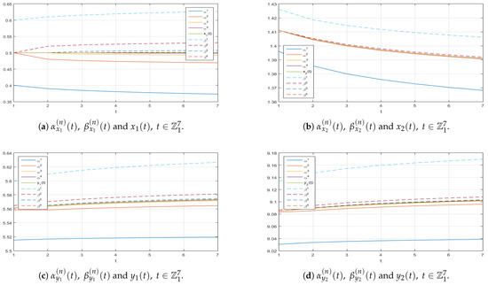
Figure A1.
Graphs along the -axis of the successive approximations and to the corresponding exact solution of (11).
Figure A1.
Graphs along the -axis of the successive approximations and to the corresponding exact solution of (11).
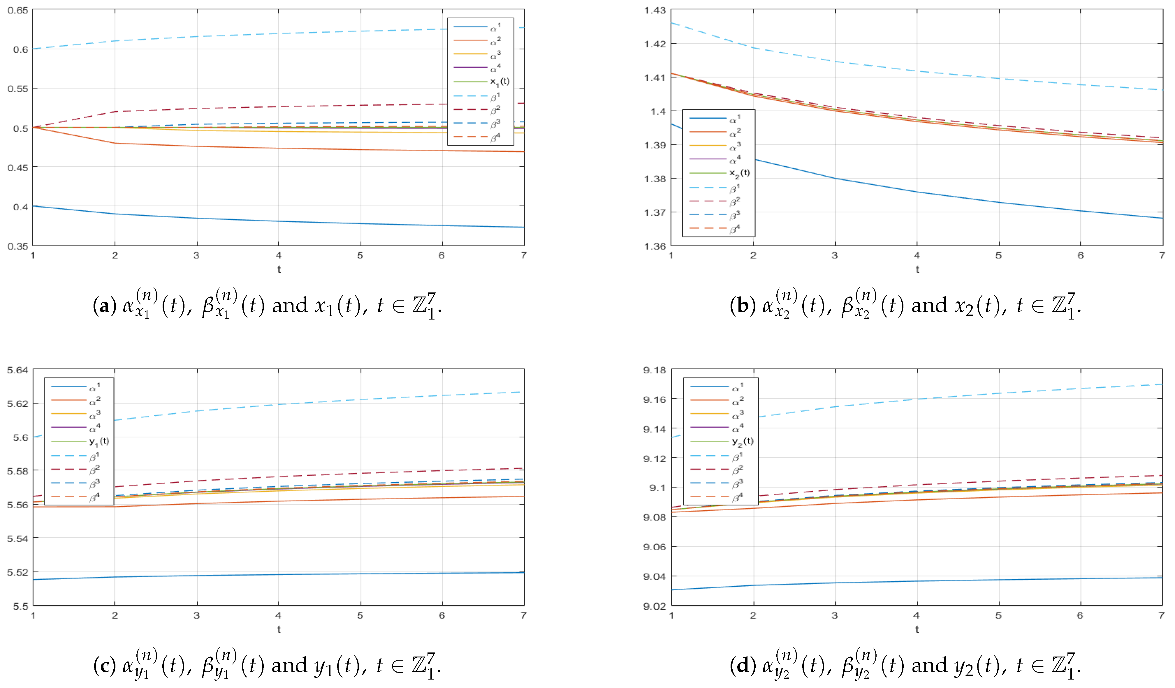
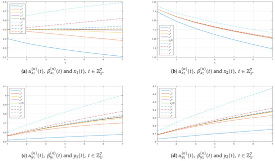
Figure A2.
Graphs along the -axis of the successive approximations and to the corresponding exact solution of (11).
Figure A2.
Graphs along the -axis of the successive approximations and to the corresponding exact solution of (11).
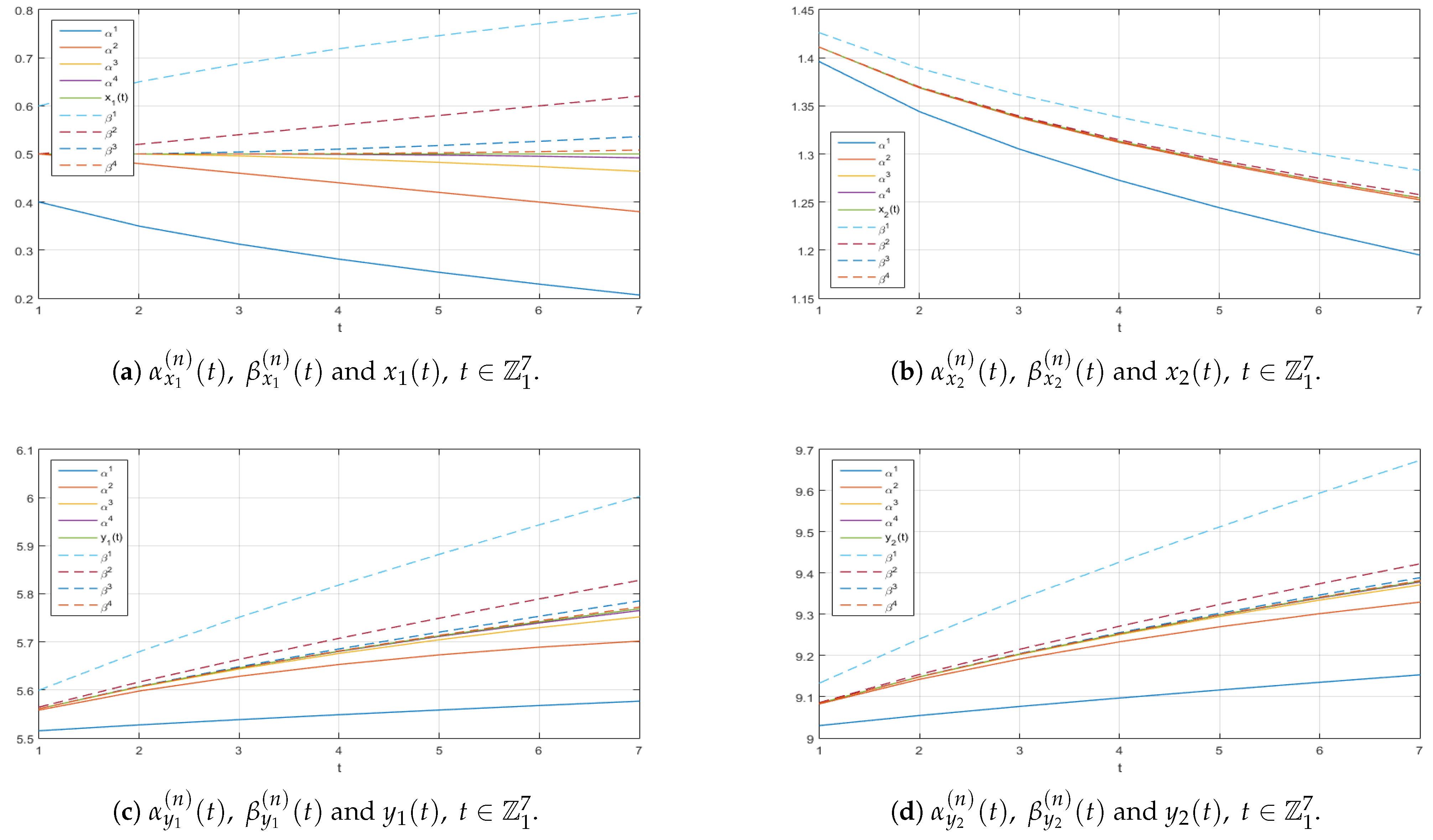
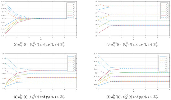
Figure A3.
Graphs along the -axis of the successive approximations and to the corresponding exact solution of (11).
Figure A3.
Graphs along the -axis of the successive approximations and to the corresponding exact solution of (11).
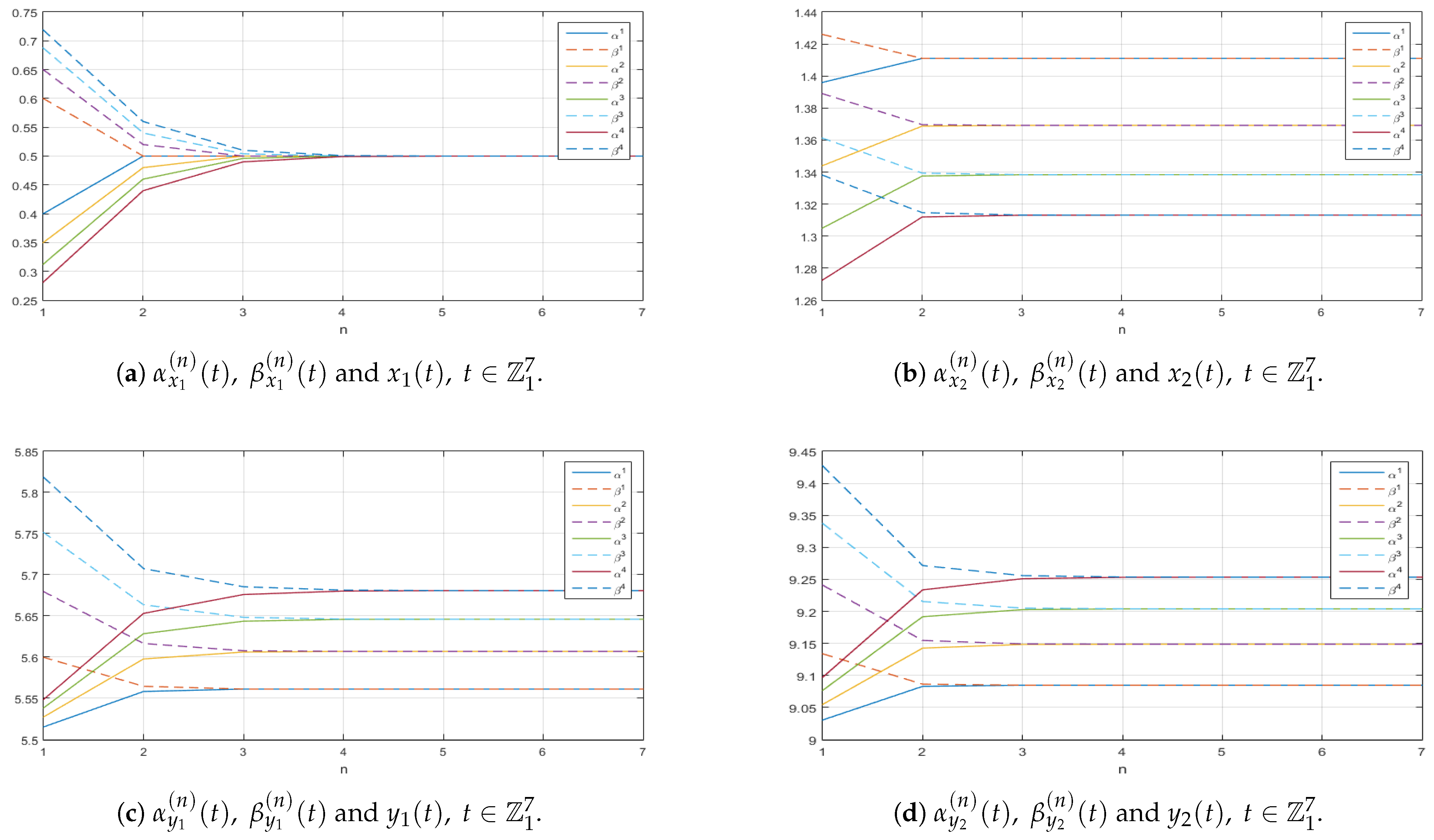
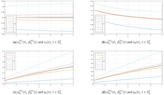
Figure A4.
Graphs along the -axis of the successive approximations and to the corresponding exact solution of (11).
Figure A4.
Graphs along the -axis of the successive approximations and to the corresponding exact solution of (11).
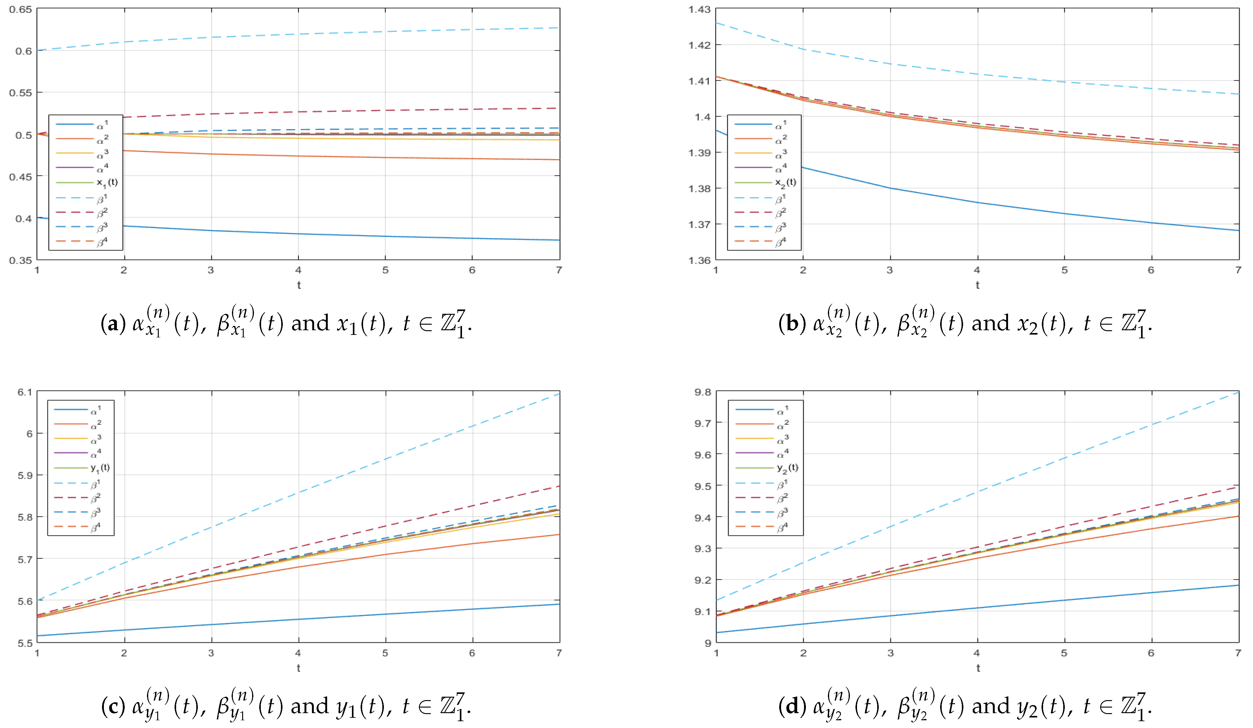
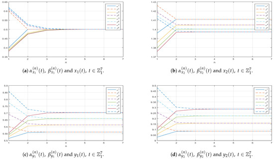
Figure A5.
Graphs along the -axis of the successive approximations and to the corresponding exact solution of (11).
Figure A5.
Graphs along the -axis of the successive approximations and to the corresponding exact solution of (11).
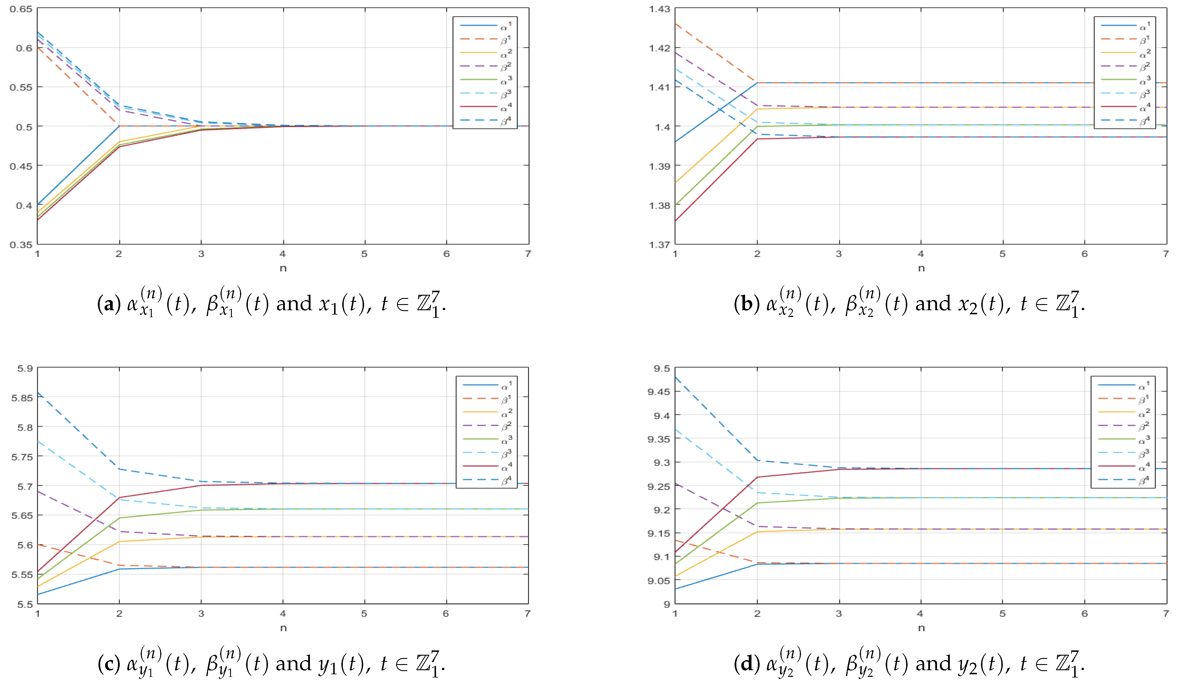
Figure A6.
Graphs along the -axis of the successive approximations and to the corresponding exact solution of (11).
Figure A6.
Graphs along the -axis of the successive approximations and to the corresponding exact solution of (11).
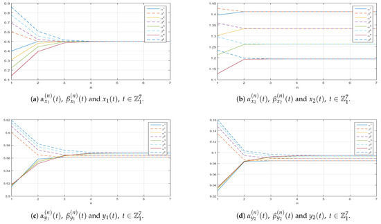
Figure A7.
Graphs along the -axis of the successive approximations and to the corresponding exact solution of (11).
Figure A7.
Graphs along the -axis of the successive approximations and to the corresponding exact solution of (11).
References
- Kilbas, A.A.; Srivastava, H.M.; Trujillo, J.J. Theory and Applications of Fractional Differential Equations; Elsevier Science BV: Amsterdam, The Netherlands, 2006. [Google Scholar]
- Podlubny, I. Fractional Differential Equation; Academic Press: San Diego, CA, USA, 1999. [Google Scholar]
- Chen, C.; Jia, B.; Liu, X.; Erbe, L. Existence and uniqueness theorem of the solution to a class of nonlinear nabla fractional difference system with a time delay. Mediterr. J. Math. 2018, 15, 1–12. [Google Scholar] [CrossRef]
- Chen, C.; Mert, R.; Jia, B.; Erbe, L.; Peterson, A. Gronwall’s inequality for a nabla fractional difference system with a retarded argument and an application. J. Differ. Equ. Appl. 2019, 25, 855–868. [Google Scholar] [CrossRef]
- Goodrich, C.S.; Peterson, A.C. Discrete Fractional Calculus; Springer: Charm, Switzerland, 2015. [Google Scholar]
- Du, F.; Jia, B. Finite-time stability of a class of nonlinear fractional delay difference systems. Appl. Math. Lett. 2019, 98, 233–239. [Google Scholar] [CrossRef]
- Damgov, V.; Trenchev, P.; Sheiretsky, K. Oscillator–wave model: Properties and heuristic instances. Chaos Solitons Fractals 2003, 17, 41–60. [Google Scholar] [CrossRef]
- Abbas, S.; Ahmad, B.; Benchohra, M.; Salim, A. Fractional Difference, Differential Equations, and Inclusions: Analysis and Stability; Morgan Kaufmann, Elsevier: Burlington, MA, USA, 2024. [Google Scholar]
- Yang, S.Y.; Wu, G.C. Discrete Gronwall’s inequality for Ulam stability of delay fractional difference equations. Math. Model. Anal. 2025, 30, 169–185. [Google Scholar] [CrossRef]
- Huang, L.L.; Park, J.H.; Wu, G.C.; Mo, Z.W. Variable-order fractional discrete-time recurrent neural networks. J. Comput. Appl. Math. 2020, 370, 112633. [Google Scholar] [CrossRef]
- Ramirez, J.D. Existence of Extremal Solutions for Caputo Fractional Differential Equations with Bounded Delay. Prog. Fract. Differ. Appl. 2023, 9, 487–498. [Google Scholar] [CrossRef]
- Hristova, S.; Stefanova, K.; Golev, A. Computer Simulation and Iterative Algorithm for Approximate Solving of Initial Value Problem for Riemann-Liouville Fractional Delay Differential Equations. Mathematics 2020, 8, 477. [Google Scholar] [CrossRef]
- Agarwal, R.; Golev, A.; Hristova, S.; O’Regan, D. Iterative techniques with computer realization for initial value problems for Riemann–Liouville fractional differential equations. J. Appl. Anal. 2020, 26, 21–47. [Google Scholar] [CrossRef]
- Agarwal, R.P.; Hristova, S.; O’Regan, D.; Almeida, R. Approximate Iterative Method for Initial Value Problem of Impulsive Fractional Differential Equations with Generalized Proportional Fractional Derivatives. Mathematics 2021, 9, 1979. [Google Scholar] [CrossRef]
- Lakshmikantham, V.; Zhang, B.G. Monotone iterative technique for delay differential equations. Appl. Anal. 1986, 22, 227–233. [Google Scholar] [CrossRef]
- Chen, C.; Bohner, M.; Jia, B. Method of upper and lower solutions for nonlinear Caputo fractional difference equations and its applications. Fract. Calc. Appl. Anal. 2019, 22, 1307–1320. [Google Scholar] [CrossRef]
- Ouncharoen, R.; Chasreechai, S.; Sitthiwirattham, T. On Nonlinear Fractional Difference Equation with Delay and Impulses. Symmetry 2020, 12, 980. [Google Scholar] [CrossRef]
- Stoenchev, M.; Todorov, V.; Georgiev, S. Notes on the Overconvergence of Fourier Series and Hadamard–Ostrowski Gaps. Mathematics 2024, 12, 979. [Google Scholar] [CrossRef]
- Madamlieva, E.; Konstantinov, M.; Milev, M.; Petkova, M. Integral Representation for the Solutions of Autonomous Linear Neutral Fractional Systems with Distributed Delay. Mathematics 2020, 8, 364. [Google Scholar] [CrossRef]
- Madamlieva, E.; Konstantinov, M. On the Existence and Uniqueness of Solutions for Neutral-Type Caputo Fractional Differential Equations with Iterated Delays: Hyers–Ulam–Mittag–Leffler Stability. Mathematics 2025, 13, 484. [Google Scholar] [CrossRef]
- Wang, M.; Jia, B.; Du, F.; Liu, X. Asymptotic stability of fractional difference equations with bounded time delays. Fract. Calc. Appl. Anal. 2020, 23, 571–590. [Google Scholar] [CrossRef]
- Hioual, A.; Ouannas, A.; Grassi, G.; Oussaeif, T.E. Nonlinear nabla variable-order fractional discrete systems: Asymptotic stability and application to neural networks. J. Comput. Appl. Math. 2023, 423, 114939. [Google Scholar] [CrossRef]
- Alzabut, J.; Tyagi, S.; Abbas, S. Discrete fractional order BAM neural networks with leakage delay: Existence and stability results. Asian J. Control 2020, 22, 143–155. [Google Scholar] [CrossRef]
- Thabet, A.; Atici, F.M. On the Definitions of Nabla Fractional Operators. Abstr. Appl. Anal. 2012, 2012, 406757. [Google Scholar] [CrossRef]
- Boulares, H.; Ardjouni, A.; Laskri, Y. Existence and uniqueness of solutions for nonlinear fractional nabla difference systems with initial conditions. Fract. Differ. Calc. 2017, 2, 247–263. [Google Scholar] [CrossRef]
- Alzabut, J.; Abdeljawad, T.; Baleanu, D. Nonlinear delay fractional difference equations with applications on discrete fractional Lotka–Volterra competition model. J. Comput. Anal. Appl. 2018, 25, 889–898. [Google Scholar]
- Abbas, S. Existence of solutions to fractional order ordinary and delay differential equations and applications. Electron. J. Differ. Equ. 2011, 9, 1–11. [Google Scholar]
- Rudin, W. Principles of Mathematical Analysis, 3rd ed.; McGraw Hill Higher Education: New York, NY, USA, 1976; ISBN 978-0070856134. [Google Scholar]
- Bogachev, V.; Smolyanov, O. Real and Functional Analysis; Springer: Cham, Switzerland, 2020. [Google Scholar] [CrossRef]
- Abdeljawad, T. On Riemann and Caputo fractional differences. Comput. Math. Appl. 2011, 62, 1602–1611. [Google Scholar] [CrossRef]
- Agarwal, R.; Golev, A.; Hristova, S.; O’Regan, D.; Stefanova, K. Iterative techniques with computer realization for the initial value problem for Caputo fractional differential equations. J. Appl. Math. Comput. 2017, 58, 433–467. [Google Scholar] [CrossRef]
- Ostalczyk, P. Discrete Fractional Calculus: Applications in Control and Image Processing; Series in Computer Vision Book 4; World Scientific: Singapore, 2015; ISBN 978-9814725668. [Google Scholar]
- Cheng, S.S. Partial Difference Equations; Advances in Discrete Mathematics and Applications; CRC Press: Boca Raton, FL, USA, 2003; Volume 3, ISBN 978-0415298841. [Google Scholar]
- Georgiev, S.; Vulkov, L. Numerical Coefficient Reconstruction of Time-Depending Integer and Fractional-Order SIR Models for Economic Analysis of COVID-19. Mathematics 2022, 10, 4247. [Google Scholar] [CrossRef]
- Georgiev, S. Mathematical Identification Analysis of a Fractional-Order Delayed Model for Tuberculosis. Fractal Fract. 2023, 7, 538. [Google Scholar] [CrossRef]
- Diethelm, K.; Ford, N.J.; Freed, A.D. A predictor-corrector approach for the numerical solution of fractional differential equations. Nonlinear Dyn. 2002, 29, 3–22. [Google Scholar] [CrossRef]
- Ghoreishi, F.; Ghaffari, R.; Saad, N. Fractional Order Runge-Kutta Methods. Fractal Fract. 2023, 7, 245. [Google Scholar] [CrossRef]
- Garrappa, R. On linear stability of predictor–corrector algorithms for fractional differential equations. Int. J. Comput. Math. 2010, 87, 2281–2290. [Google Scholar] [CrossRef]
- Lubich, C. Discretized fractional calculus. SIAM J. Math. Anal. 1986, 17, 704–719. [Google Scholar] [CrossRef]
- Wu, G.C.; Baleanu, D.; Huang, L.L. Novel Mittag-Leffler stability of linear fractional delay difference equations with impulse. Appl. Math. Lett. 2018, 82, 71–78. [Google Scholar] [CrossRef]
- Liu, H.; Zhao, L. Ground-state solution of a nonlinear fractional Schrödinger–Poisson system. Math. Methods Appl. Sci. 2022, 45, 1934–1958. [Google Scholar] [CrossRef]
- Lv, W. Existence of solutions for discrete fractional boundary value problems with a p-Laplacian operator. Adv. Differ. Equ. 2012, 2012, 163. [Google Scholar] [CrossRef]
- Liu, H.; Jin, Y.; Hou, C. Existence of positive solutions for discrete delta-nabla fractional boundary value problems with p-Laplacian. Bound. Value Probl. 2017, 2017, 60. [Google Scholar] [CrossRef]
- Zhang, W.; Zhai, C. Positive solutions for a Riemann-Liouville fractional system with ρ-Laplacian operators. Differ. Equ. Appl. 2024, 16, 305–319. [Google Scholar] [CrossRef]
- Han, Z.; Lu, H.; Zhang, C. Positive solutions for eigenvalue problems of fractional differential equation with generalized p-Laplacian. Appl. Math. Comput. 2015, 257, 526–536. [Google Scholar] [CrossRef]

Disclaimer/Publisher’s Note: The statements, opinions and data contained in all publications are solely those of the individual author(s) and contributor(s) and not of MDPI and/or the editor(s). MDPI and/or the editor(s) disclaim responsibility for any injury to people or property resulting from any ideas, methods, instructions or products referred to in the content. |
© 2025 by the authors. Licensee MDPI, Basel, Switzerland. This article is an open access article distributed under the terms and conditions of the Creative Commons Attribution (CC BY) license (https://creativecommons.org/licenses/by/4.0/).