Abstract
High-order methods are particularly crucial for achieving highly accurate solutions or satisfying high-order optimality conditions. However, most existing high-order methods require solving complex high-order Taylor polynomial models, which pose significant computational challenges. In this paper, we propose a Chebyshev–Halley method with gradient regularization, which retains the convergence advantages of high-order methods while effectively addressing computational challenges in polynomial model solving. The proposed method incorporates a quadratic regularization term with an adaptive parameter proportional to a certain power of the gradient norm, thereby ensuring a closed-form solution at each iteration. In theory, the method achieves a global convergence rate of or even , attaining the optimal rate of third-order methods without requiring additional acceleration techniques. Moreover, it maintains local superlinear convergence for strongly convex functions. Numerical experiments demonstrate that the proposed method compares favorably with similar methods in terms of efficiency and applicability.
Keywords:
Chebyshev–Halley method; quadratic regularization; gradient norm; closed-form solution; global convergence; local superlinear convergence MSC:
49M37; 90C25; 90C30; 68Q25
1. Introduction
In this paper, we consider the following unconstrained convex optimization problem:
where is a continuously differentiable function with a globally Lipschitz continuous third-order derivative.
From a theoretical standpoint, high-order optimization methods exploit th-order derivative information to attain enhanced convergence rates compared to first- and second-order methods. Furthermore, in the context of non-convex optimization, these methods exhibit a distinct advantage of circumventing degenerate solutions induced by singular Hessian matrices, thereby yielding solutions with higher precision and superior quality [1,2]. The modern development of high-order methods can be traced back to the cubic regularization of Newton’s method (CNM) [3], which laid the foundation for subsequent extensions to pth-order tensor methods [4,5,6,7,8], as well as adaptive [9,10,11,12] and stochastic [13,14,15,16] variants. In the aforementioned studies, a pth-order Taylor polynomial model is employed to approximate the objective function at :
where is the ith-order derivative and is the ith-order derivative along . The next iterate is updated as , where , and it continues until a satisfactory solution is found.
The non-convex nature of the polynomial model presents a significant challenge for these methods in achieving minimization. Nesterov [17] demonstrated that a sufficiently large regularization parameter can ensure the convexity of the model while preserving the theoretical advantages of local high-order approximations, particularly in settings where the ith-order derivative is Lipschitz continuous. Furthermore, Nesterov developed an efficient minimization scheme for a convex polynomial model with , incorporating a linearly convergent inner iteration at each step. The scheme leverages automatic differentiation techniques [18,19] to compute third-order derivatives along specific directions, significantly improving computational efficiency. Doikov et al. [20] proposed an inexact strategy for tensor methods, which initially reduced the accuracy of the model’s solution and gradually improved it in later iterations, thus ensuring global convergence. Cartis et al. [21] utilized the cubic-quartic regularization (CQR) framework to successfully address the minimization of a non-convex cubic model with quartic regularization. Ahmadi et al. [22] introduced sum-of-squares (SoS) convex polynomials as an alternative to address the limitations of the Taylor model in intuitive representation, and they solved the resulting model via n-dimensional semidefinite programming. Subsequently, ref. [23] integrated SoS into an adaptive framework, extending its applicability to general non-convex problems. Xiao et al. [24] proposed a regularized Chebyshev–Halley method (RCH) for solving a third-order polynomial model, achieving a global convergence rate of , which can be further accelerated to . The method transforms the solution of a polynomial model into the simultaneous resolution of a regularized Newton equation and a Halley equation, while maintaining computational complexity comparable to that of second-order methods.
Another active line of research aims to improve convergence rates through acceleration techniques. In machine learning and deep learning applications, for example, efficient methods not only accelerate model convergence but also significantly reduce computational resource requirements. In this context, two primary directions have been explored. The first is Nesterov-type acceleration [17,25,26,27], which leverages the estimate sequence technique. However, this technique relies on intricate algebraic constructions, leading to a lack of a unified mathematical explanation for its acceleration mechanism. Furthermore, experimental studies have indicated that accelerated tensor methods may underperform in practice [28]. The second direction is based on the accelerated hybrid proximal extragradient (A-HPE) framework [29,30,31,32], which achieves an optimal convergence rate of for pth-order optimization methods. Despite its theoretical advantages, this framework requires multiple iterative sequences, additional hyperparameters, and a time-consuming bisection line search process that is sensitive to parameter choices, making it less suitable for high-dimensional problems.
In practical scenarios, researchers tend to prefer fundamental methods due to their simplicity, ease of implementation, and generalizability to various optimization problems. Polyak [33] introduced a quadratic regularization technique in his work and proposed the following iterative scheme:
where . This iteration is concise and admits a closed-form solution at each step, circumventing the need to solve the polynomial model , but it only achieves the global convergence rate. Ueda et al. [34] employed a similar technique and reconstructed the quadratic Taylor polynomial model as follows:
Although its minimization leads to the same iterative scheme, the global convergence rate remains suboptimal. The aforementioned studies suggest that the quadratic regularization strategy may establish a balance between computational efficiency and global convergence, offering a new pathway for developing fundamental methods.
Recently, Doikov et al. [35] combined quadratic regularization with the Bregman distance, designing a regularization parameter . The resulting regularized Newton method can be viewed as a generalized relaxation of CNM, which theoretically not only preserves the global convergence rate of but also significantly reduces the computational complexity through closed-form iterations. Mishchenko [36] explored the relationship between the Levenberg–Marquardt penalty and CNM, constructing a quadratic regularization model. Despite differences in theoretical analysis, the proposed method achieves the same convergence rate and also admits a closed-form solution. Building on this, ref. [37] further unified quadratic and cubic regularization forms while introducing novel regularization terms such as the elastic net. Refs. [38,39,40,41] have also explored simple methods for more general or non-convex problems. Meanwhile, significant progress has been made in fundamental methods based on stepsize adjustment. Hanzely et al. [42,43] designed a novel damping parameter update scheme for the damped Newton method by revealing the implicit duality between the Newton stepsize and Levenberg–Marquardt regularization. This scheme updates the stepsize using the product of the gradient and the Hessian matrix, achieving a global convergence rate of or .
In this paper, we propose a Chebyshev–Halley method with gradient regularization, a third-order method that combines rapid convergence with iterative simplicity. The proposed method employs a quadratic regularization strategy, where the regularization parameter is adjusted based on a power of the gradient norm at the current iterate. Therefore, the iterate is updated directly through matrix inversion and vector multiplication, which removes the need for nested inner iterations to solve the polynomial model. Theoretically, the method can achieve a global convergence rate of or without requiring acceleration techniques, attaining the optimal convergence rate for third-order methods. Numerical experiments demonstrate its effectiveness and applicability across various scenarios.
2. Gradient-Regularized Chebyshev–Halley Method
For , define , and , where and represent the gradient, Hessian matrix, and third-order derivative, respectively. The objective function is assumed to satisfy the following standard conditions.
Assumption 1.
The objective function is convex and differentiable on , with a Lipschitz continuous third-order derivative. Specifically, there exists a constant such that for any ,
As a direct consequence, for any , the following bounds hold:
These bounds in (2) and (3) quantify the approximation errors of the gradient and Hessian, respectively, and play a crucial role in analyzing the convergence behavior of the proposed method.
Assumption 2.
The level set is bounded, satisfying
The classical Chebyshev–Halley method, also known as the improved hyperbolic tangent method, is iteratively formatted as [44] , where , are the solutions to the Newton equation
and the Halley equation
respectively. To improve the global convergence of the method, ref. [24] approximate using a third-order Taylor polynomial model with a quartic regularization term and incorporate an acceleration sequence to achieve a global convergence rate of . However, this method requires nested inner iterations to solve the model, and the introduction of an acceleration sequence further complicates parameter tuning.
In this section, we consider the following third-order Taylor polynomial model with quadratic regularization:
where , is a regularization parameter proportional to a certain power of the gradient norm at . The basic iterative framework of the algorithm is presented below.
Algorithm 1 incorporates a quadratic regularization term and third-order derivatives to enhance convergence properties. The quadratic regularization term ensures global convergence while also providing a closed-form solution, thereby avoiding the need for nested inner iterations to solve the high-order Taylor polynomial model. Simultaneously, the utilization of the third-order derivative accelerates convergence, and the computational cost of third-order derivatives is comparable to that of Newton’s method [45].
| Algorithm 1 Chebyshev–Halley method with gradient regularization (CHGR). |
Require: Initial point , , and .
|
We now derive an upper bound for the regularized Newton direction.
Corollary 1.
Suppose that Assumption 1 holds. Thus,
In particular, if , then
Define . From (6) and (7), it follows that
Furthermore, assuming that there exists a constant such that , then, combining (9) and the norm triangle inequality, we obtain
Thus, and are of the same order of magnitude, meaning that is primarily determined by , while serves only as a secondary correction term, proportional to the square of . As approaches zero, the effect of diminishes, making its contribution to the overall stepsize negligible.
3. Convergence Analysis
This section is dedicated to analyzing the convergence of the proposed method. We begin by estimating the bound for the third-order derivative along the direction .
Lemma 1.
Suppose that Assumption 1 holds. For any and , we have
Proof.
For any , it follows from (3) that
Let , where and with . Then,
By dividing both sides of the inequality by and taking the norm, we obtain
By minimizing the right-hand side of the inequality with respect to , we obtain the optimal parameter . Substituting into the inequality above yields the upper bound (11). □
Lemma 2.
Suppose that Assumption 1 holds. For any , we have
Proof.
The following theorem establishes the descent property of the objective function, ensuring that each iteration sufficiently reduces the gradient norm.
Theorem 1.
Suppose that Assumption 1 holds and that the regularization parameter satisfies
where , . Then, we have
Proof.
From (2) and (7), we obtain
Squaring both sides of the above inequality yields
By using the Cauchy–Schwarz inequality and the norm triangle inequality, we obtain
and
By substituting these inequalities into (15) and using , we obtain
By combining (8), (10)–(12), we obtain
and
Thus, we obtain
To ensure that (14) holds, we divide into five parts, each satisfying the following conditions:
- (i).
- , which leads to .
- (ii).
- , which leads to .
- (iii).
- , which leads to .
- (iv).
- , which leads to .
- (v).
- , which leads to .
By combining these conditions, we obtain the requirement (13). Thus, the theorem is proven. □
Based on the previous results, we now establish the global convergence of the proposed method.
Theorem 2.
Suppose that Assumptions 1–2 hold. Thus, the sequence generated by the Algorithm 1 satisfies
Proof.
From Assumption 2, for any , we have
which implies
where D is the bound of the level set .
For and , the function is concave. Consequently, we have
Let . By combining this with (14), we obtain
Let . Thus,
where the first inequality follows from (18), the second inequality follows from (19), and the third inequality follows from (17). By setting and using the fact that , the above inequality is simplified to
By summing these inequalities from 1 to k, we obtain
where the second inequality follows from the geometric–arithmetic mean inequality, and the third inequality follows from (17).
As , the inequality does not hold. Therefore, we have
which implies
Thus, the first case in (16) is proven.
Let and . Following a similar derivation process, the second case in (16) can be proven. □
In Algorithm 1, we set . Based on the convergence analysis, we know that can be chosen as or . Correspondingly, the value of H is given by , or .
Next, we investigate the local convergence of the proposed method.
Theorem 3.
Suppose that Assumption 1 holds and that is a -strongly convex function on . If there exists a constant such that for all , , where is a sufficiently small positive constant, then
Proof.
From the strong convexity of , it follows that
By combining (14), we obtain
Further, by combining (2) and the first-order optimality condition of Model (4), we have
where the third inequality follows from (22), the fourth inequality follows from (8), and the last inequality follows from Corollary 1. □
Under the strong convexity condition, most existing works (e.g., refs. [34,35,36,37,38]) have established the local quadratic convergence of various Newton-type methods. However, the third-order method proposed in this paper exhibits a faster convergence rate, achieving an order of , where .
4. Numerical Experiments
In this section, we evaluate the performance of CHGR (Algorithm 1) on two classical test problems: -regularized logistic regression and log-sum-exp. The experiments compare CHGR with various gradient-regularized methods, including the regularized Newton method (RegN [35,36]), the super-universal Newton method (SUN [39]), CNM [3] and RCH [24]. Additionally, we focus on several damped Newton methods with simple iterations and reliable global convergence properties, such as the affine-invariant cubic Newton method (AICN [42]) and the root Newton stepsize schedule (RN [43]). All numerical experiments were conducted in the MATLAB R2019b environment on a laptop equipped with an Intel Core i7 processor and 8GB of memory. Table 1 summarizes the iteration schemes and global convergence properties of the aforementioned methods.

Table 1.
Summary of iteration schemes and convergence properties for third-order methods ().
The following two problems are widely used in the fields of optimization and machine learning, commonly employed to evaluate the effectiveness and robustness of optimization algorithms in practical tasks.
Problem 1.
-regularized logistic regression:
where are the given data samples, with representing the feature vectors and representing the class label. is the regularization coefficient that controls model complexity and prevents overfitting. If is too small, it may result in ill-conditioned problems, negatively affecting the stability and convergence of the methods.
The experiments are conducted on datasets provided by LIBSVM (https://www.csie.ntu.edu.tw/~cjlin/libsvmtools/datasets/, accessed on 14 April 2025), including the ionosphere, mushroom, a4a, and a9a datasets. All linear systems are solved using the MATLAB backslash operator “∖”. The initial point for AICN and RN is chosen as [42,43], while the initial points for the remaining methods are randomly generated from a standard normal distribution. The termination criterion for all methods is set as , and H is selected to be either or . To evaluate the adaptability of the methods under different regularization strengths, is set to or .
Problem 2.
log-sum-exp:
where the components of vectors and are independently sampled from a uniform distribution over the interval . The parameter is a smoothing factor that controls the approximation accuracy. This function serves as a smooth approximation of . When ρ is small, the function becomes poorly conditioned.
In the experiments, the initial points for all methods are generated from a standard normal distribution, with the initial parameter set as . The termination criterion is set as . To comprehensively evaluate the performance of the methods, two problem sizes are tested: and . Additionally, different smoothing parameters are selected to assess the convergence stability of the methods.
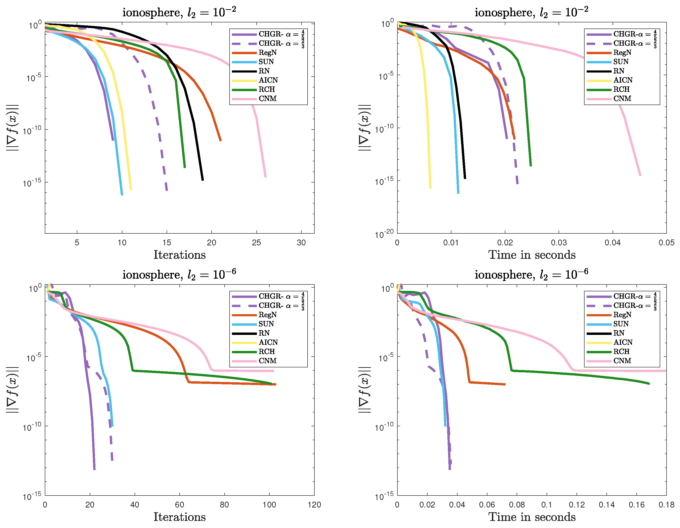
Figure 1, Figure 2, Figure 3 and Figure 4 illustrate the performance comparison of the methods on Problem 1. The detailed analysis is as follows:
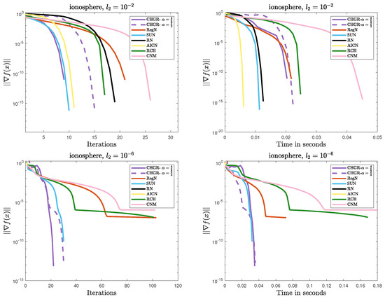
Figure 1.
Performance comparison of the methods on Problem 1 (ionosphere: ).

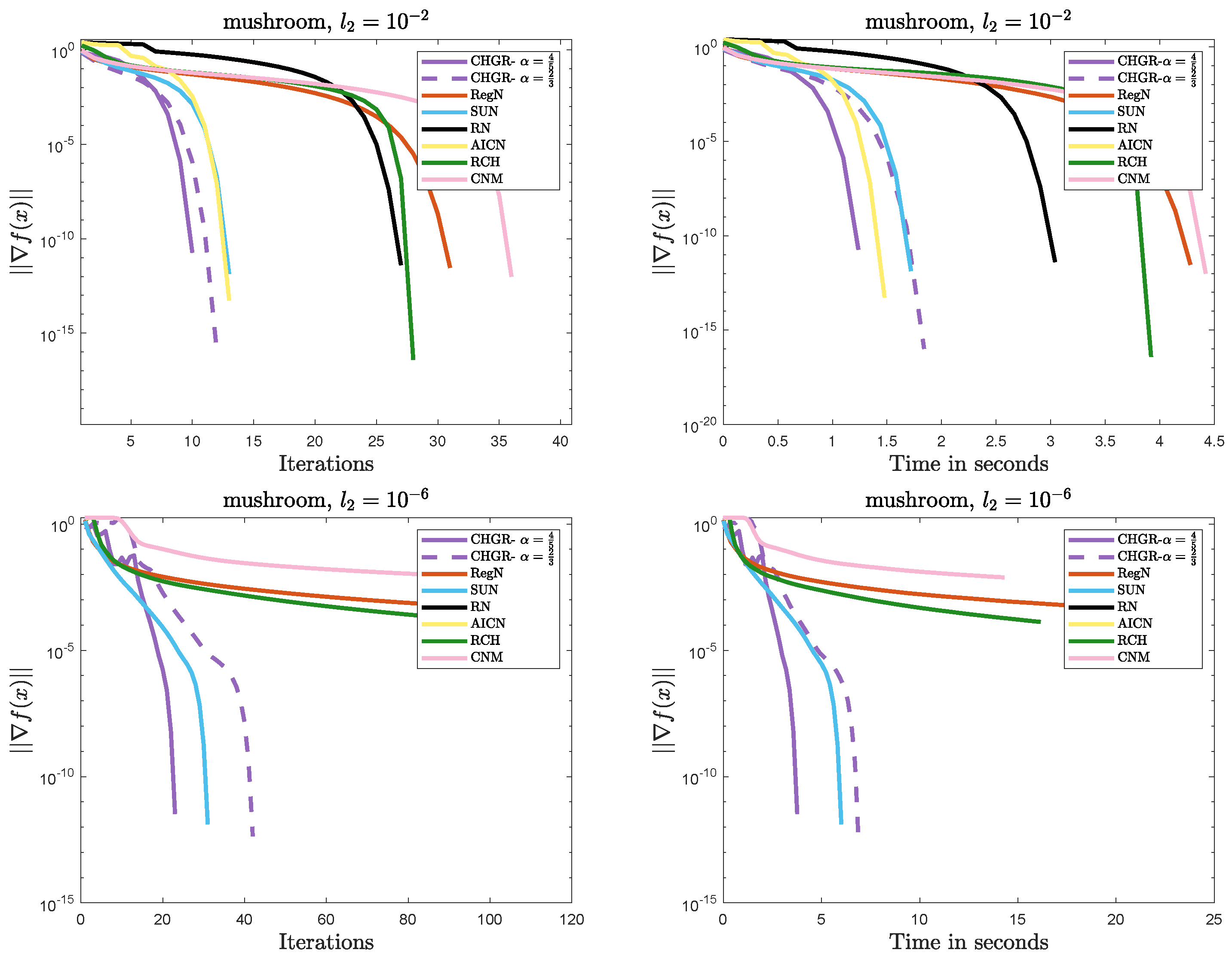
Figure 2.
Performance comparison of the methods on Problem 1 (mushroom: ).
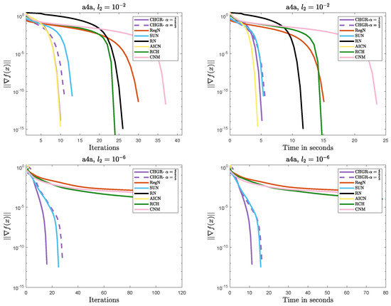
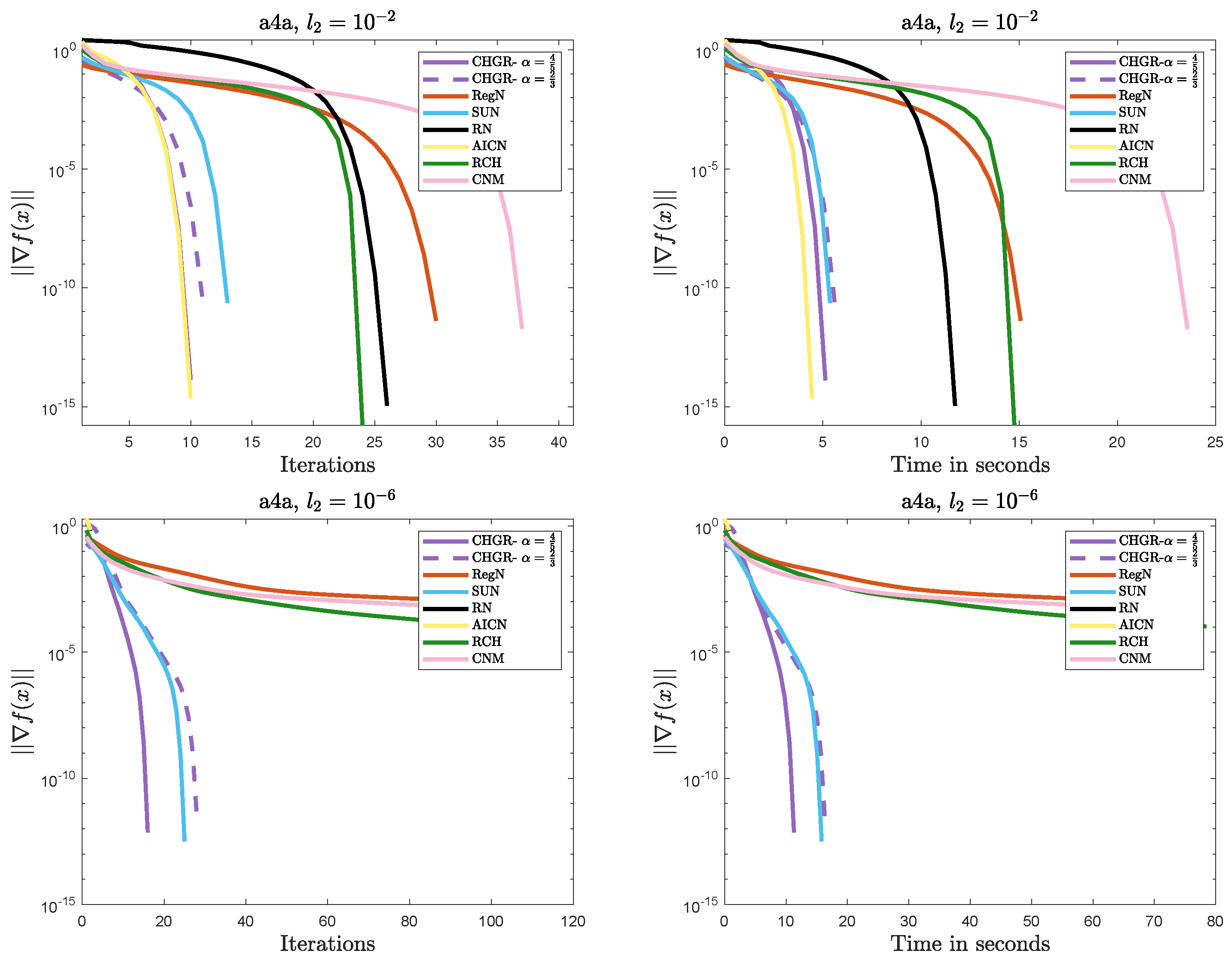
Figure 3.
Performance comparison of the methods on Problem 1 (a4a: ).
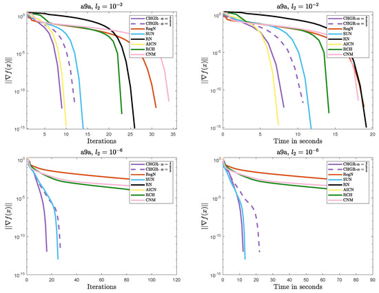
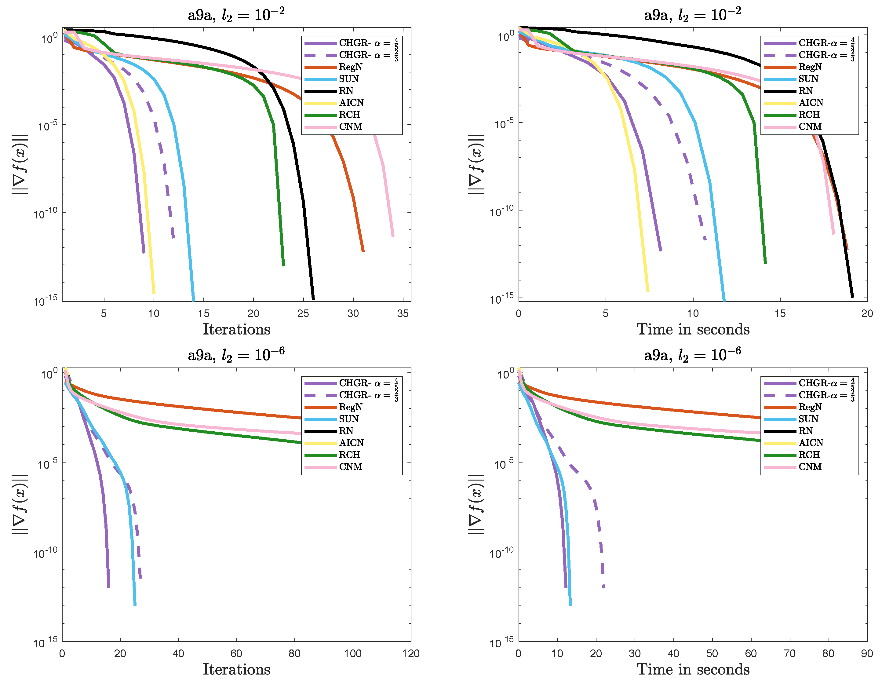
Figure 4.
Performance comparison of the methods on Problem 1 (a9a: ).
- Efficient Convergence
- –
- In most cases, CHGR performs best with , which is consistent with theoretical results. In terms of both iteration count and computational efficiency, CHGR significantly outperforms second-order methods such as AICN, RN, RegN, and CNM. This is due to its two-step iterative framework, which accelerates convergence by incorporating third-order derivative information while maintaining computational complexity comparable to that of second-order methods.
- –
- For , AICN has a slightly less or comparable computational time to CHGR, due to fewer matrix and vector multiplication operations. However, for , AICN fails after only two steps of a normal iteration due to its high sensitivity to parameters. A similar issue also occurs in RN.
- –
- For , CHGR outperforms SUN in terms of the computational time on a9a () but performs slightly worse on a4a (). SUN is a single-step Newton iteration with an adaptive update strategy for , and it can accelerate convergence in some cases. However, the need to verify the descent condition for the adaptive strategy introduces additional computational costs.
- Numerical Stability
- –
- CHGR maintains stable convergence across different regularization strengths, while CNM and RCH fail to achieve satisfactory solutions within 100 steps for . This may be due to the more flexible regularization strategy of CHGR, which dynamically adjusts the regularization parameter based on the gradient norm, thereby improving convergence.
- –
- For , AICN and CHGR exhibit comparable performance. However, for , the weaker regularization causes the problem to become ill-conditioned, leading to the failure of AICN and RN to converge. Additionally, these two methods are more sensitive to the initial point, often failing due to numerical instability when initialized with or a random initialization.
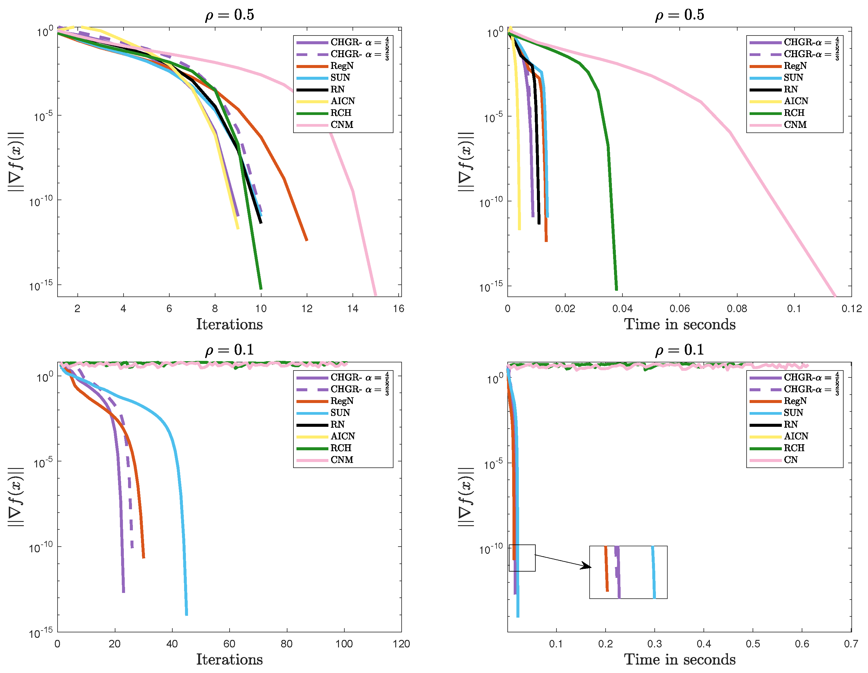
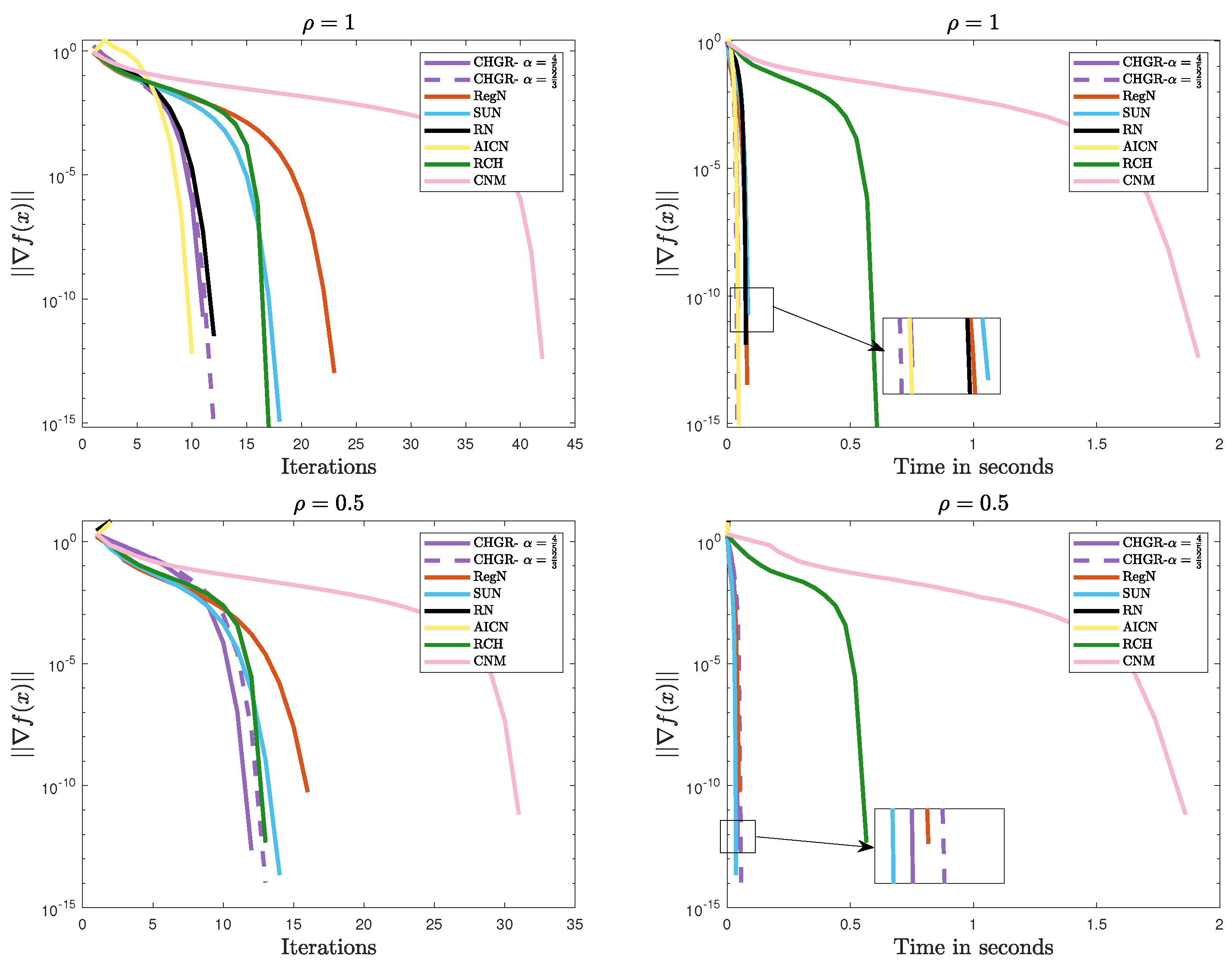
Figure 5 and Figure 6 present the comparative results of the methods on Problem 2. The experimental results demonstrate that CHGR consistently achieves fast and stable convergence, showcasing its excellent convergence performance and strong adaptability to various problems. In comparison, AICN and RN succeed only when the problem is well conditioned, failing to converge for ill-conditioned cases like or . Additionally, CNM and RCH also diverge for , , indicating their limitations in handling ill-conditioned problems.
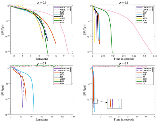
Figure 5.
Performance comparison of the methods on Problem 2 ().
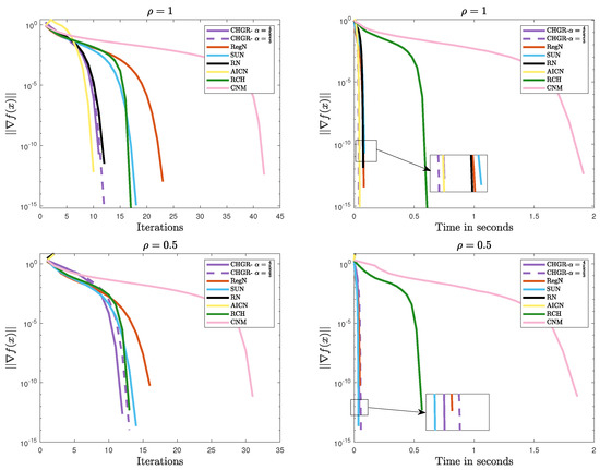
Figure 6.
Performance comparison of the methods on Problem 2 ().
In summary, CHGR demonstrates excellent convergence and numerical stability across various test problems and different regularization strengths, indicating its strong flexibility and applicability in handling complex problems.
5. Results
This paper proposes a Chebyshev–Halley method with gradient regularization, which demonstrates excellent global convergence properties while maintaining iteration simplicity. The method employs a third-order Taylor polynomial model with a quadratic regularization term and adjusts the regularization parameter based on a power of the gradient norm. In each iteration, the method requires only matrix inversion and vector products to obtain a closed-form solution, avoiding the complexity of nested sub-iterations for solving the polynomial model. Despite not incorporating acceleration techniques, the method theoretically achieves a global convergence rate of or and exhibits locally superlinear convergence for strongly convex problems. Numerical experiments show that the proposed method outperforms gradient-regularized Newton-type methods, such as RegN and SUN. Moreover, it exhibits greater adaptability than damped Newton methods like AICN and RN.
Author Contributions
Methodology, software, formal analysis and writing—original draft preparation: J.X.; methodology, funding Acquisition and supervision: H.Z.; formal analysis, writing—review and editing, funding acquisition: H.G. All authors have read and agreed to the published version of the manuscript.
Funding
This work was supported by the National Science Foundation of China (Grant No. 12471295, Grant No. 12171145) and the Training Program for Excellent Young Innovators of Changsha (Grant No. kq2209021).
Data Availability Statement
No new data were created or analyzed in this study.
Conflicts of Interest
The authors declare no conflicts of interest.
References
- Anandkumar, A.; Ge, R. Efficient approaches for escaping higher order saddle points in non-convex optimization. In Proceedings of the 29th Annual Conference on Learning Theory, New York, NY, USA, 23–26 June 2016; pp. 81–102. [Google Scholar]
- Chen, X.; Toint, P.L. High-order evaluation complexity for convexly-constrained optimization with non-Lipschitzian group sparsity terms. Math. Program. 2021, 187, 47–78. [Google Scholar] [CrossRef]
- Nesterov, Y.; Polyak, B.T. Cubic regularization of Newton method and its global performance. Math. Program. 2006, 108, 177–205. [Google Scholar] [CrossRef]
- Baes, M. Estimate Sequence Methods: Extensions and Approximations; Institute for Operations Research, ETH: Zürich, Switzerland, 2009; Volume 2. [Google Scholar]
- Gould, N.I.M.; Rees, T.; Scott, J.A. A Higher Order Method for Solving Nonlinear Least-Squares Problems; RAL Preprint RAL-P-2017–010; STFC Rutherford Appleton Laboratory: Oxfordshire, UK, 2017. [Google Scholar]
- Calandra, H.; Gratton, S.; Riccietti, E.; Vasseur, X. On high-order multilevel optimization strategies. SIAM J. Optimiz. 2021, 31, 307–330. [Google Scholar] [CrossRef]
- Jiang, B.; Wang, H.; Zhang, S. An optimal high-order tensor method for convex optimization. Math. Oper. Res. 2021, 46, 1390–1412. [Google Scholar] [CrossRef]
- Ahookhosh, M.; Nesterov, Y. High-order methods beyond the classical complexity bounds: Inexact high-order proximal-point methods. Math. Program. 2024, 208, 365–407. [Google Scholar] [CrossRef] [PubMed]
- Cartis, C.; Gould, N.I.M.; Toint, P.L. Adaptive cubic regularisation methods for unconstrained optimization. Part I: Motivation, convergence and numerical results. Math. Program. 2011, 127, 245–295. [Google Scholar] [CrossRef]
- Cartis, C.; Gould, N.I.M.; Toint, P.L. Adaptive cubic regularisation methods for unconstrained optimization. Part II: Worst-case function-and derivative-evaluation complexity. Math. Program. 2011, 130, 295–319. [Google Scholar] [CrossRef]
- Jiang, B.; Lin, T.; Zhang, S. A unified adaptive tensor approximation scheme to accelerate composite convex optimization. SIAM J. Optimiz. 2020, 30, 2897–2926. [Google Scholar] [CrossRef]
- Grapiglia, G.N.; Nesterov, Y. Adaptive third-order methods for composite convex optimization. SIAM J. Optimiz. 2023, 33, 1855–1883. [Google Scholar] [CrossRef]
- Chen, X.; Jiang, B.; Lin, T.; Zhang, S. Accelerating adaptive cubic regularization of Newton’s method via random sampling. J. Mach. Learn. Res. 2022, 23, 1–38. [Google Scholar]
- Lucchi, A.; Kohler, J. A sub-sampled tensor method for nonconvex optimization. IMA J. Numer. Anal. 2023, 43, 2856–2891. [Google Scholar] [CrossRef]
- Agafonov, A.; Kamzolov, D.; Dvurechensky, P.; Gasnikov, A.; Takáč, M. Inexact tensor methods and their application to stochastic convex optimization. Optim. Methods Softw. 2024, 39, 42–83. [Google Scholar] [CrossRef]
- Zhao, J.; Doikov, N.; Lucchi, A. Cubic regularized subspace Newton for non-convex optimization. In Proceedings of the 28th International Conference on Artificial Intelligence and Statistics, Phuket, Thailand, 3–5 May 2025. [Google Scholar]
- Nesterov, Y. Implementable tensor methods in unconstrained convex optimization. Math. Program. 2021, 186, 157–183. [Google Scholar] [CrossRef]
- Griewank, A. A mathematical view of automatic differentiation. Acta Numer. 2003, 12, 321–398. [Google Scholar] [CrossRef]
- Zhang, H.; Deng, N. An improved inexact Newton method. J. Glob. Optim. 2007, 39, 221–234. [Google Scholar] [CrossRef]
- Doikov, N.; Nesterov, Y.E. Inexact Tensor Methods with Dynamic Accuracies. In Proceedings of the 37th International Conference on Machine Learning, Virtual Event, 13–18 July 2020; pp. 2577–2586. [Google Scholar]
- Cartis, C.; Zhu, W. Cubic-quartic regularization models for solving polynomial subproblems in third-order tensor methods. Math. Program. 2025, 1–53. [Google Scholar] [CrossRef]
- Ahmadi, A.A.; Chaudhry, A.; Zhang, J. Higher-order newton methods with polynomial work per iteration. Adv. Math. 2024, 452, 109808. [Google Scholar] [CrossRef]
- Cartis, C.; Zhu, W. Global Convergence of High-Order Regularization Methods with Sums-of-Squares Taylor Models. arXiv 2024, arXiv:2404.03035. [Google Scholar]
- Xiao, J.; Zhang, H.; Gao, H. An Accelerated Regularized Chebyshev–Halley Method for Unconstrained Optimization. Asia Pac. J. Oper. Res. 2023, 40, 2340008. [Google Scholar] [CrossRef]
- Nesterov, Y. Accelerating the cubic regularization of Newton’s method on convex problems. Math. Program. 2008, 112, 159–181. [Google Scholar] [CrossRef]
- Nesterov, Y. Inexact accelerated high-order proximal-point methods. Math. Program. 2023, 197, 1–26. [Google Scholar] [CrossRef]
- Kamzolov, D.; Pasechnyuk, D.; Agafonov, A.; Gasnikov, A.; Takáč, M. OPTAMI: Global Superlinear Convergence of High-order Methods. arXiv 2024, arXiv:2410.04083. [Google Scholar]
- Antonakopoulos, K.; Kavis, A.; Cevher, V. Extra-newton: A first approach to noise-adaptive accelerated second-order methods. NeurIPS 2022, 35, 29859–29872. [Google Scholar]
- Monteiro, R.D.C.; Svaiter, B.F. An accelerated hybrid proximal extragradient method for convex optimization and its implications to second-order methods. SIAM J. Optimiz. 2013, 23, 1092–1125. [Google Scholar] [CrossRef]
- Birgin, E.G.; Gardenghi, J.L.; Martínez, J.M.; Santos, S.A.; Toint, P.L. Worst-case evaluation complexity for unconstrained nonlinear optimization using high-order regularized models. Math. Program. 2017, 163, 359–368. [Google Scholar] [CrossRef]
- Gould, N.I.M.; Rees, T.; Scott, J.A. Convergence and evaluation-complexity analysis of a regularized tensor-Newton method for solving nonlinear least-squares problems. Comput. Optim. Appl. 2019, 73, 1–35. [Google Scholar] [CrossRef]
- Huang, Z.; Jiang, B.; Jiang, Y. Inexact and Implementable Accelerated Newton Proximal Extragradient Method for Convex Optimization. arXiv 2024, arXiv:2402.11951. [Google Scholar]
- Polyak, R.A. Regularized Newton method for unconstrained convex optimization. Math. Program. 2009, 120, 125–145. [Google Scholar] [CrossRef]
- Ueda, K.; Yamashita, N. A regularized Newton method without line search for unconstrained optimization. Comput. Optim. Appl. 2014, 59, 321–351. [Google Scholar] [CrossRef]
- Doikov, N.; Nesterov, Y. Gradient regularization of Newton method with Bregman distances. Math. Program. 2024, 204, 1–25. [Google Scholar] [CrossRef]
- Mishchenko, K. Regularized Newton method with global O(1/k2) convergence. SIAM J. Optimiz. 2023, 33, 1440–1462. [Google Scholar] [CrossRef]
- Yamakawa, Y.; Yamashita, N. Convergence analysis of a regularized Newton method with generalized regularization terms for unconstrained convex optimization problems. Appl. Math. Comput. 2025, 491, 129219. [Google Scholar] [CrossRef]
- Jiang, Y.; He, C.; Zhang, C.; Ge, D.; Jiang, B.; Ye, Y. Beyond Nonconvexity: A Universal Trust-Region Method with New Analyses. arXiv 2023, arXiv:2311.11489. [Google Scholar]
- Doikov, N.; Mishchenko, K.; Nesterov, Y. Super-universal regularized newton method. SIAM J. Optimiz. 2024, 34, 27–56. [Google Scholar] [CrossRef]
- Gratton, S.; Jerad, S.; Toint, P.L. Yet another fast variant of Newton’s method for nonconvex optimization. IMA J. Numer. Anal. 2025, 45, 971–1008. [Google Scholar] [CrossRef]
- Zhou, Y.; Xu, J.; Bao, C.; Ding, C.; Zhu, J. A Regularized Newton Method for Nonconvex Optimization with Global and Local Complexity Guarantees. arXiv 2025, arXiv:2502.04799. [Google Scholar]
- Hanzely, S.; Kamzolov, D.; Pasechnyuk, D.; Gasnikov, A.; Richtárik, P.; Takác, M. A Damped Newton Method Achieves Global and Local Quadratic Convergence Rate. NeurIPS 2022, 35, 25320–25334. [Google Scholar]
- Hanzely, S.; Abdukhakimov, F.; Takáč, M. Damped Newton Method with Near-Optimal Global O(k−3) Convergence Rate. arXiv 2024, arXiv:2405.18926. [Google Scholar]
- Jackson, R.H.F.; McCormick, G.P. The polyadic structure of factorable function tensors with applications to high-order minimization techniques. J. Optimiz. Theory Appl. 1986, 51, 63–94. [Google Scholar] [CrossRef]
- Zhang, H. On the Halley class of methods for unconstrained optimization problems. Optim. Methods Softw. 2010, 25, 753–762. [Google Scholar] [CrossRef]
Disclaimer/Publisher’s Note: The statements, opinions and data contained in all publications are solely those of the individual author(s) and contributor(s) and not of MDPI and/or the editor(s). MDPI and/or the editor(s) disclaim responsibility for any injury to people or property resulting from any ideas, methods, instructions or products referred to in the content. |
© 2025 by the authors. Licensee MDPI, Basel, Switzerland. This article is an open access article distributed under the terms and conditions of the Creative Commons Attribution (CC BY) license (https://creativecommons.org/licenses/by/4.0/).