Price Decisions in a Two-Server Queue Considering Customer Retrial Behavior: Profit-Driven Versus Social-Driven

Abstract

This study investigates price decisions in a queue with two servers, where customers exhibit retrial behavior. There is no waiting space. Arrival customers have the option to either join the system or balk; when the two servers are occupied, those who decide to enter become repeat customers. Two scenarios where the waiting lines in orbit are unobservable and observable are considered. We analyze customers’ behavior and derive their Nash equilibrium strategies under both cases. Additionally, we examine optimal pricing decisions aimed at maximizing profit and social welfare, respectively. Moreover, we demonstrate that these objectives often lead to divergent outcomes. Compared to a single-server queue, the reduction in customers’ sojourn time is more obvious when the waiting line is unobservable. Under certain conditions—such as a large potential market size, high customer impatience, or a low retrial rate—increasing the number of service personnel can enhance both profit and social welfare. Notably, a profit-maximizing manager is more incentivized to increase servers than the social planner. These findings provide valuable insights for balancing operational efficiency, profitability, and customer satisfaction in queue management systems.

1. Introduction and Literature Review

Researchers have widely adopted a queuing model as a fundamental framework for modeling congested service/production systems, with extensive studies focusing on the development and analysis of operational strategies to enhance system performance optimization (e.g., Lai et al. [1], Samanta and Rashmi [2]). In congestion-prone service or production systems, it is common for servers or producers to be occupied when customers arrive. In such scenarios, the customers whose needs are not immediately met generally make an attempt after a stochastic waiting period. Aissani [3] highlights that the advancement of information technology has significantly amplified customers’ retrial behavior. This behavior can have profound implications, including increased energy consumption and a potential decline in service quality (Tapiero [4]). For theoretical research in such systems, the primary emphasis lies on assessing performance and tackling control issues by stochastic processes and dynamic programming methodologies (Dimitriou [5]). Artalejo and Gómez-Corral [6] as well as Falin and Templeton [7] provide comprehensive overviews.

1.1. Motivation

Generally, customers can make their own decisions. Several studies have explored retrial queues from an economic perspective (e.g., Economou and Kanta [8]; Cui et al. [9]), where managers address optimization problems by considering customer behavior. In queue systems, a widely adopted strategy to enhance retrial customers’ satisfaction and loyalty is to increase the number of service personnel. For instance, in call centers, deploying multiple servers can significantly reduce customer wait times and improve satisfaction levels (Armony and Maglaras [10]). However, since multi-server systems entail higher operational costs, managers often opt for a two-server configuration (Tang et al. [11]). A practical example can be observed in amusement parks, where two ticket check channels—server-assisted and self-checkout—are typically available. Customers who need to check receive immediate service if at least one channel is free. However, if both channels are occupied, the customer may leave temporarily, perhaps to grab a refreshment, and return later to retry. Given that pricing is a critical tool for managing demand and maximizing profit, how should a manager of a two-server system set prices when dealing with customers’ retrial behavior? Do socially optimal prices align with profit-maximizing prices? Furthermore, is increasing a server always advantageous for the system? A significant research gap exists in the literature regarding the interplay between customers’ queuing behavior and the economic analysis of these systems, which motivates this work.

1.2. Literature Review

Our research is in line with the economic analysis of service/production systems that are modeled as queuing systems. In the pioneering study of this area, Naor [12] assumes that customers strategically decide to join or balk. Through analysis, he obtains customers’ equilibrium thresholds under such observable circumstances. Similarly, Edelson and Hilderbrand [13] identify the corresponding equilibrium strategy for an unobservable case. Both studies also delve into pricing decisions. Naor [12] demonstrates that the revenue-maximizing price diverges from the welfare-maximizing one in an observable case, while Edelson and Hilderbrand [13] show that these prices coincide if the queue length is unobservable. For additional details, readers are directed to the exhaustive reviews by Hassin and Haviv [14] and Hassin [15].

Several researchers have conducted economic analyses of multi-server systems. Hassin and Haviv [16] explore a two-server system where customers strategically select the shorter queue based on available system state information or randomly select a queue without such information. This study derives equilibrium policies. Hassin [17] examines a two-server queuing configuration with dedicated queues. Customers can observe the queue length in one service channel, while the other remains unobservable. The study addresses whether an observable queue consistently attracts a higher share of demand compared to an unobservable one. In a two-server system, Zhao and Wang [18] reveal that introducing a line-sitting service can significantly enhance throughput. Zhou et al. [19] investigate the interactions between private and public service providers and derive their respective optimal pricing strategies. Cattani and Schmidt [20] find that in multi-server systems, concealing the queue length information and pooling dedicated queues can alleviate congestion, reducing metrics such as average waiting time and queue length. In a two-server system with a single queue, Tang et al. [11] establish the equilibrium queuing strategies for customers in an unobservable scenario involving two distinct customer types. In addition, Yechiali [21] and Wang et al. [22] analyze customers’ joining rules in multi-server queuing systems, providing further insights into customer behavior and system performance.

A queuing system that incorporates customer retrial behavior is referred to as a retrial queue, and several studies have examined it from an economic perspective. Early contributions to this field include Kulkarni [23], Elcan [24], and Hassin and Haviv [25]. These studies concentrate on a retrial queue where there is only one server, examining the equilibrium retrial rate by assuming that balking is prohibited. For scenarios where customers’ balking behavior is allowed, Economou and Kanta [8] derive customers’ equilibrium strategies for both unobservable and observable queues in the context of a single-server configuration. Furthermore, they tackle the associated pricing problems with the target of maximizing both profit and social welfare. In a retrial model, Wang and Zhang [26] examine the equilibrium strategies adopted by customers within the framework of the classic retrial policy. Cui et al. [9] show that, by incorporating retrial costs in an observable retrial queue, the availability of the retry option can result in a decrease in customer welfare when compared to a system where retrial behavior is absent. Further studies have investigated operational strategies for various retrial queuing systems by incorporating additional features, such as information heterogeneity (Wang and Zhang [27]) or customers’ bounded rationality (Zhang and Wang [28]). Nevertheless, all aforementioned studies investigate single-server systems. This gap in the literature motivates our investigation into the economic and operational analysis of two-server retrial systems.

Since pricing is a critical factor influencing customers’ decisions, a key operational question arises: How should a manager set prices in a two-server system to effectively respond to customer behavior? How do these pricing strategies differ from those in a single-server queue? Existing studies have not fully addressed these questions, leaving gaps in the literature. We extend the work of Economou and Kanta [8] to a two-server system. This study explores customers’ retrial behavior and derives their equilibrium strategies. Furthermore, it examines pricing strategies from both the perspective of a profit-seeking server as well as that of a social planner. By addressing these issues, our research provides valuable insights into managing operations in service or production systems that encounter retrial customers, offering practical guidance for balancing profitability and customer satisfaction.

The structure of this study is as follows: The assumptions are outlined in Section 2. Section 3 formulates customers’ equilibrium strategies and examines pricing decisions in the context of an unobservable queue, followed by a parallel analysis for the observable case. Section 4 provides numerical examples to illustrate the theoretical findings. Lastly, Section 5 concludes this study by summarizing the primary findings and insights obtained. All proofs are provided in Appendix A.

2. Introduction

There is a service or production system with two identical servers, i.e., the two servers have the same service speed. This system does not have any waiting areas. Arrivals of potential customers follow a Poisson process with a rate of $\lambda$. Upon arrival, the customers who find at least one available server immediately receive the service. However, if the two servers are busy, they can choose whether to retry or not. We suppose that those customers who decide to retry join an orbit. The server, once it becomes idle, will seek a customer from this orbit. The time required to find a customer in orbit is assumed to be exponentially distributed with rate $\theta$. During the seeking process, a new customer may arrive. In this case, the server interrupts the seeking process and serves the new customer. The service time is exponentially distributed with service rate $\mu$. It is assumed that all parameters are independent of each other. This model is referred to as a two-server constant retrial queue.

Denote R as the reward a customer receives upon completing the service. During the sojourn time—which includes both the time in the service area and orbit—customers have a waiting cost of c per unit of time, and they need to pay a price P after the service is completed. When there is an idle server, to encourage customers to join, we suppose

$$R-P-{\displaystyle \frac{c}{\mu }}>0.$$

(1)

If this fails to be met, all potential customers will decline to join, even when servers are idle; thus, the system’s profit will be zero. What is more, once a customer’s decision is made, it is irrevocable.

Let $I\left(t\right)$ denote the server state where

$$I\left(t\right)=\left\{\begin{array}{c}0,\mathrm{if}\mathrm{two}\mathrm{servers}\mathrm{are}\mathrm{idle}\mathrm{at}\mathrm{time}t;\hfill \\ 1,\mathrm{if}\mathrm{only}\mathrm{one}\mathrm{server}\mathrm{is}\mathrm{idle}\mathrm{at}\mathrm{time}t;\hfill \\ 2,\mathrm{if}\mathrm{two}\mathrm{servers}\mathrm{are}\mathrm{busy}\mathrm{at}\mathrm{time}t.\hfill \end{array}\right.$$

At an arbitrary time epoch t, $N\left(t\right)$ denotes the number of customers in the retrial orbit. The system states at any time t are described by a bi-variate stochastic process $\left\{I\right(t),N(t\left)\right\}$ with state space $\{0,1,2\}\times \{0,1,2,\cdots \}$.

3. Analysis of Customers’ Equilibrium Behavior and Optimal Price

We examine two distinct information scenarios: unobservable and observable. In both scenarios, incoming customers are informed about the current status of the servers (whether they are available or occupied). In the observable case, customers can also observe the exact number of customers waiting in orbit. By contrast, they will not obtain it in the unobservable case. This difference in information availability influences customers’ decisions.

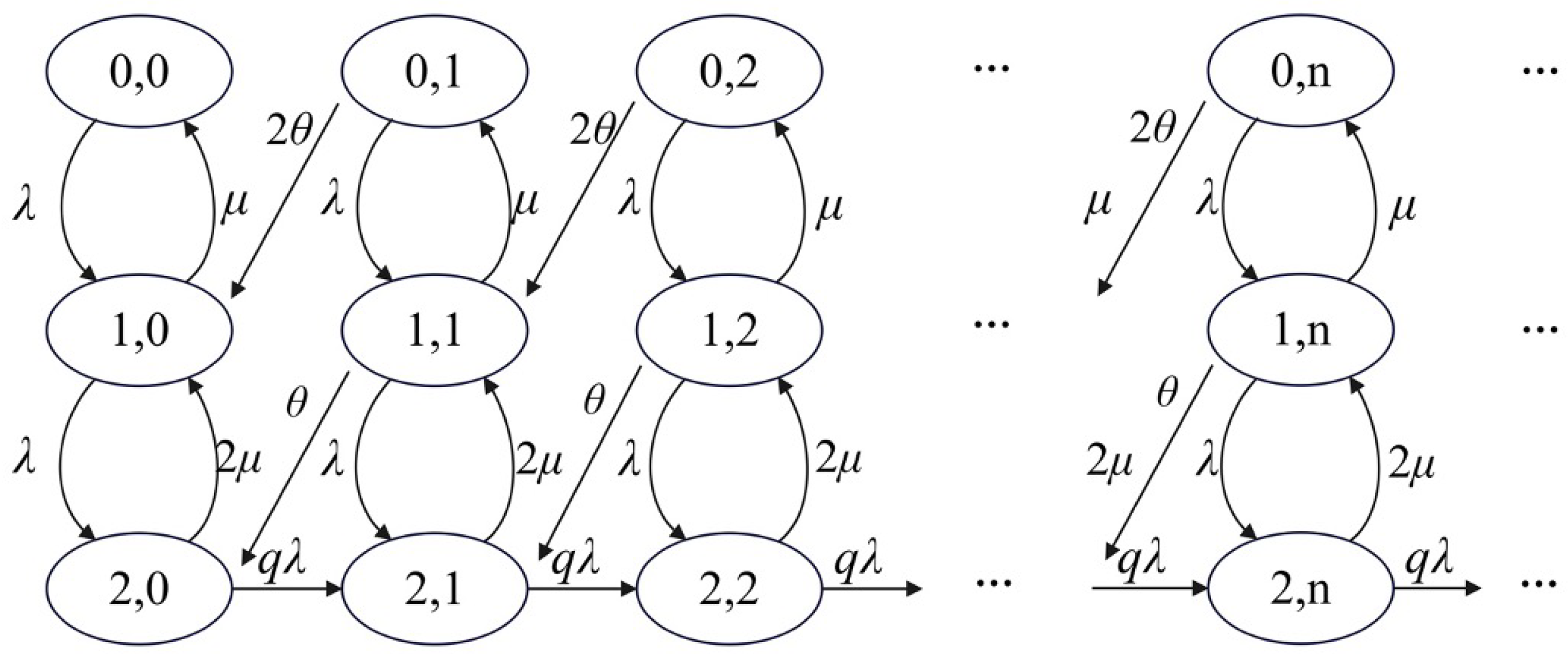
3.1. The Unobservable Case

In this information scenario, based on the model assumptions and Equation (1), arriving customers will join the system, provided that there is at least one idle server. We now concentrate on customers’ join-or-balk decisions when both servers are occupied. Since customers cannot observe the real-time queue length of retrial customers already in orbit, we assume that they opt to join the retrial orbit with a probability of q and balk with the complementary probability. The system operates similarly to the original one, but the arrival rate is $\lambda q$ when both servers are occupied. Figure 1 presents the transition diagram for this case.

Let $p(i,j)$ denote the steady-state probability for state $(i,j)$. We can define $p_i\left(z\right)={\displaystyle \sum _{j=0}^{\infty }}{z}^{j}p(i,j),i=0,1,2$ as its partial generating functions.

Lemma 1. 

In an unobservable two-server constant retrial queue, arriving customers will join the system if an idle server is available and will enter orbit with probability q if both servers are occupied. If $q\lambda (\lambda +\theta )(\lambda +2\theta )<2\theta \mu (\lambda +2\theta +2\mu )$, the system reaches a stable state. The stationary probabilities for the states—both servers are idle, only one server is idle, and both servers are busy—are as follows:

$$\begin{array}{cc}\hfill & p_0\left(1\right)={\displaystyle \frac{\theta [\psi \left(q\right)-2q{\lambda }^2]}{\sqrt{\varphi \left(q\right)}}}p(0,0),p_1\left(1\right)={\displaystyle \frac{\lambda \theta \psi \left(q\right)}{\mu \sqrt{\varphi \left(q\right)}}}p(0,0),p_2\left(1\right)={\displaystyle \frac{{\lambda }^2\theta (\lambda +2\theta +2\mu )}{\mu \sqrt{\varphi \left(q\right)}}}p(0,0),\hfill \end{array}$$

where $\varphi \left(q\right)={[2\theta \mu (\lambda +2\theta +2\mu )-q\lambda (\lambda +\theta )(\lambda +2\theta )]}^2$ and $\psi \left(q\right)=2\mu (\lambda +2\theta +2\mu )-q\lambda (\lambda +2\theta )$. The average number of customers in the retrial orbit for these three states are, respectively, given by

$$\begin{array}{cc}\hfill & N_0={\displaystyle \frac{2q{\lambda }^3\theta \mu (\lambda +2\theta +2\mu +q\lambda )}{\varphi \left(q\right)}}p(0,0),N_1={\displaystyle \frac{2q{\lambda }^3\theta (\lambda +2\theta )(\lambda +2\theta +2\mu +q\lambda )}{\varphi \left(q\right)}}p(0,0),\hfill \\ \hfill & N_2={\displaystyle \frac{q{\lambda }^3\theta (\lambda +2\theta +2\mu )[(\lambda +\theta )(\lambda +2\theta )+2\theta \mu ]}{\mu \varphi \left(q\right)}}p(0,0).\hfill \end{array}$$

Here, $p(0,0)={\displaystyle \frac{\mu \left[2\theta \mu \right(\lambda +2\theta +2\mu )-q\lambda (\lambda +\theta \left)\right(\lambda +2\theta \left)\right]}{\theta \{(\lambda +2\theta +2\mu )[{\lambda }^2(1-q)+2\lambda \mu +2{\mu }^2]-q\lambda \mu (\lambda +2\theta )\}}}$.

Customers make decisions relying on a function that takes into account the reward, the price they pay, and the expected waiting time. Initially, we derive customers’ expected sojourn time. When tagging a customer in orbit, $T(i,j)$ represents this customer’s expected sojourn time, given that they are at the j-th position in orbit and the server is in state $i(=0,1,2)$. The following lemma offers insights into their expected sojourn times.

Lemma 2. 

In the context of an unobservable two-server constant retrial queue, if $q\lambda (\lambda +\theta )(\lambda +2\theta )<2\theta \mu (\lambda +2\theta +2\mu )$ and there are $j-1$ other customers waiting in orbit, the expected sojourn times  $T(i,j)$ for state  $i(=0,1,2)$ until service begins for the tagged customer are provided by

$$\begin{array}{cc}\hfill & T(0,j)=\xi j+{\displaystyle \frac{(\lambda +2\theta )(\theta +\mu )}{\mu (\lambda +2\theta +2\mu )(\lambda +2\theta )}},T(1,j)=\xi j+{\displaystyle \frac{1}{\mu }},T(2,j)=\xi j+{\displaystyle \frac{3}{2\mu }}.\hfill \end{array}$$

Here,  $\xi ={\displaystyle \frac{2\mu (\lambda +2\theta +\mu )+(\lambda +\theta )(\lambda +2\theta )}{2\theta \mu (\lambda +2\theta +2\mu )}}$ . When both servers are occupied, the expected sojourn time for arriving customers, whose joining probability is q, is given by

$$\begin{array}{cc}\hfill W_u\left(q\right)=& {\displaystyle \frac{3}{2\mu }}-{\displaystyle \frac{1}{\lambda +2\theta +2\mu }}-{\displaystyle \frac{2\mu (\lambda +2\theta +\mu )}{(\lambda +2\theta +2\mu )(\lambda +\theta )(\lambda +2\theta )}}\hfill \\ \hfill & +\left[{\displaystyle \frac{2\mu (\lambda +2\theta +\mu )}{(\lambda +\theta )(\lambda +2\theta )}}+1\right]{\displaystyle \frac{2\theta \mu +(\lambda +\theta )(\lambda +2\theta )}{\sqrt{\varphi \left(q\right)}}}.\hfill \end{array}$$

Obviously, $W_u\left(q\right)$ is increasing in q.

Clearly, $T(i,j)$ varies with the server’s state i. If the stable condition changes into

$$\begin{array}{c}\hfill {\displaystyle \frac{\lambda (\lambda +\theta )(\lambda +2\theta )}{2\theta \mu (\lambda +2\theta +2\mu )}}<1,\end{array}$$

(2)

this indicates that the original system, which does not incorporate customers’ decision-making processes, is stable. Consequently, the system remains stable under any strategy q. The conclusions regarding the scenario where Condition (2) is not satisfied can be readily derived from this case, as we will elaborate later.

As discussed in Economou and Kanta [8], if the tagged customer finds that two servers are busy, his reward–cost function is

$$U_u\left(q\right)=R-P-c{W}_u\left(q\right).$$

Based on this, we can outline the strategies employed by customers.

Theorem 1. 

In the unobservable two-server constant retrial queue in which Conditions (1) and (2) hold, given price P, an incoming customer will enter certainly if an idle server is available, and they will enter with a probability $q_e$ if both servers are occupied. $q_e$ is

$$\begin{array}{c}\hfill q_e=\left\{\begin{array}{c}0,ifP\ge R-c{W}_u\left(0\right),\hfill \\ q^{*}\in (0,1),ifR-c{W}_u\left(1\right)<P<R-c{W}_u\left(0\right),\hfill \\ 1,ifP\le R-c{W}_u\left(1\right),\hfill \end{array}\right.\end{array}$$

where $q^{*}={\displaystyle \frac{2\theta \mu (\lambda +2\theta +2\mu )}{\lambda (\lambda +\theta )(\lambda +2\theta )}}-{\displaystyle \frac{\frac{2\theta \mu +(\lambda +\theta )(\lambda +2\theta )}{\lambda (\lambda +\theta )(\lambda +2\theta )}\left(\frac{2\mu (\lambda +2\theta +\mu )}{(\lambda +\theta )(\lambda +2\theta )}+1\right)}{\frac{R-P}{c}-\frac{3}{2\mu }+\frac{1}{\lambda +2\theta +2\mu }+\frac{2\mu (\lambda +2\theta +\mu )}{(\lambda +2\theta +2\mu )(\lambda +\theta )(\lambda +2\theta )}}}$.

As demonstrated in this theorem, price plays a critical role in influencing customers’ decisions. They may join or balk as the price varies.

Remark 1. 

If Condition (2) does not hold but $q\lambda (\lambda +\theta )(\lambda +2\theta )<2\theta \mu (\lambda +2\theta +2\mu )$ holds, the probability $q_e$ is

$$\begin{array}{c}\hfill q_e=\left\{\begin{array}{c}0,ifP\ge R-c{W}_u\left(0\right),\hfill \\ q^{*}\in (0,1),ifR-c{W}_u\left(1\right)<P<R-c{W}_u\left(0\right).\hfill \end{array}\right.\end{array}$$

3.1.1. Profit-Maximizing Price in the Unobservable Case

Theorem 1 delineates customers’ equilibrium strategies. In this subsection, we broaden our analysis to ascertain the price that maximizes profit. For a given price P, the system’s profit function per unit of time is formulated as

$$\begin{array}{c}\hfill {\Pi }_u\left(P\right)={\lambda }^{*}\left(P\right)P,\end{array}$$

(3)

where ${\lambda }^{*}\left(P\right)$ represents the effective arrival rate.

$$\begin{array}{cc}\hfill {\lambda }^{*}\left(P\right)& =\lambda \left(p_0\left(1\right)+p_1\left(1\right)\right)+q_e\left(P\right)\lambda p_2\left(1\right)\hfill \\ \hfill & ={\displaystyle \frac{\lambda \mu \left[2(\lambda +\mu )(\lambda +2\theta +2\mu )-q_e\left(P\right)\lambda (\lambda +2\theta )\right]}{(\lambda +2\theta +2\mu )\left[{\lambda }^2(1-q_e\left(P\right))+2\lambda \mu +2{\mu }^2\right]-q_e\left(P\right)\lambda \mu (\lambda +2\theta )}}.\hfill \end{array}$$

There is an extreme case where $q_e=0$. When $P\ge R-c{W}_u\left(0\right)$, $q_e=0$. The profit function of this scenario can be rewritten as

$$\begin{array}{c}\hfill {\Pi }_u\left(P\right)={\displaystyle \frac{2\lambda \mu (\lambda +\mu )}{{\lambda }^2+2\lambda \mu +2{\mu }^2}}P.\end{array}$$

(4)

We define the optimal price as $P^m$. According to (4), $P^m$ is determined by a value that closely approximates $R-{\displaystyle \frac{c}{\mu }}$.

To encourage customers to join the orbit, the price should fulfill $P<R-c{W}_u\left(0\right)$. Since $R-c{W}_u\left(1\right)$ may be less than 0, the analysis falls into $R-c{W}_u\left(1\right)\ge 0$ and $R-c{W}_u\left(1\right)<0$. If the price falls within the interval $\left[max\left\{0,R-c{W}_u\left(1\right)\right\},R-c{W}_u\left(0\right)\right)$, it always has $q_e>0$.

Theorem 2. 

In the unobservable two-server constant retrial queue where Conditions (1) and (2) hold, the optimal price $P_u=argmax\{{\Pi }_u\left(P\right), P\in \{max\left\{0,R-c{W}_u\left(1\right)\right\}, P^{*}, P^m\}\}$, where $P^{*}\in (max\{0,R-c{W}_u\left(1\right)\}, R-c{W}_u\left(0\right))$ is the unique solution of $P{\displaystyle \frac{d{\lambda }^{*}\left(P\right)}{dP}}+{\lambda }^{*}\left(P\right)=0$.

The optimal price may be achieved in three cases. When arriving customers find two servers busy, the three cases are all potential customers, part of the potential customers, and no customer choosing to retry. Different pricing structures create varying incentives for customer retrial decisions.

Remark 2. 

If Condition (2) does not hold but $q\lambda (\lambda +\theta )(\lambda +2\theta )<2\theta \mu (\lambda +2\theta +2\mu )$ holds, the optimal price $P_u=argmax\left\{{\Pi }_u\left(P\right),P\in \left\{P^{*},P^m\right\}\right\}$.

3.1.2. Welfare-Maximizing Price in the Unobservable Case

Social welfare encompasses both the surplus of customers and servers. Given a price P and a joining probability q when customers find two busy servers, the respective surpluses per unit time for customers and servers are as follows:

$$\begin{array}{cc}\hfill & {CS}_u\left(P\right)=\lambda \left(p_0\left(1\right)+p_1\left(1\right)\right)\left(R-P-{\displaystyle \frac{c}{\mu }}\right)+q\lambda p_2\left(1\right)\left(R-P-c{W}_u\left(q\right)\right),\hfill \\ \hfill & {SS}_u\left(P\right)=\lambda \left(p_0\left(1\right)+p_1\left(1\right)+q{p}_2\left(1\right)\right)P.\hfill \end{array}$$

Therefore, the social welfare per unit of time is

$$\begin{array}{c}\hfill {SW}_u\left(q\right)=\lambda \left(p_0\left(1\right)+p_1\left(1\right)\right)\left(R-{\displaystyle \frac{c}{\mu }}\right)+q\lambda p_2\left(1\right)\left(R-c{W}_u\left(q\right)\right).\end{array}$$

(5)

Theorem 3. 

In the unobservable two-server constant retrial queue in which Conditions (1) and (2) hold, an incoming customer will enter the system certainly (Probability 1) upon finding an idle server. If the two servers are busy, the socially optimal strategy $q_u$ is

$$\begin{array}{c}\hfill q_u=\left\{\begin{array}{c}0,ifR<c{H}_3,\hfill \\ x_1, ifc{H}_3\le R<cH,\hfill \\ 1, ifR\ge cH.\hfill \end{array}\right.\end{array}$$

In the above statements,

$$\begin{array}{cc}\hfill & x_1={\displaystyle \frac{-E-\sqrt{E^2-4DF}}{2D}},H_3={\displaystyle \frac{1}{\mu }}+{\displaystyle \frac{{\Delta }_3}{2\theta {\mu }^2[(\lambda +\theta )(\lambda +2\theta )+4\mu (\lambda +\mu )]}},\hfill \\ \hfill & H={\displaystyle \frac{1}{\mu }}+{\displaystyle \frac{{\lambda }^2{\Delta }_1-2\lambda \theta (\lambda +2\theta +2\mu ){\Delta }_2+2\theta \mu {(\lambda +2\theta +2\mu )}^2{\Delta }_3}{\mu [(\lambda +2\theta )(\lambda +2\mu )+4\mu (\lambda +\mu )]{[2\theta \mu a-\lambda (\lambda +\theta )(\lambda +2\theta )]}^2}},\hfill \\ \hfill & D={\lambda }^2\{(\lambda +\theta ){(\lambda +2\theta )}^2(R\mu -c)[(\lambda +2\theta )(\lambda +2\mu )+4\mu (\lambda +\mu )]-c{\Delta }_1\},\hfill \\ \hfill & E=-2\lambda \theta (\lambda +2\theta +2\mu )\{2\mu (\lambda +\theta )(\lambda +2\theta )(R\mu -c)[(\lambda +2\theta )(\lambda +2\mu )+4\mu (\lambda +\mu )]-c{\Delta }_2\},\hfill \\ \hfill & F=2\theta \mu {(\lambda +2\theta +2\mu )}^2\{2\theta \mu (R\mu -c)[(\lambda +2\theta )(\lambda +2\mu )+4\mu (\lambda +\mu )]-c{\Delta }_3\},\hfill \\ \hfill & {\Delta }_1=\lambda (\lambda +\theta ){(\lambda +2\theta )}^2\left({\displaystyle \frac{\lambda (\lambda +2\theta )}{2\mu }}-2\mu \right)\hfill \\ \hfill & -2\mu (\lambda +\theta )(\lambda +2\theta )(\lambda +2\theta +\mu )({\lambda }^2+2\lambda \mu +2{\mu }^2)\hfill \\ \hfill & -2\mu \left[\right(\lambda +\mu \left)\right(\lambda +2\theta )+2\lambda \mu ]\left[\right(\lambda +\theta \left)\right(\lambda +2\theta \left)\right(\lambda +3\theta +\mu )+2\theta \mu (\lambda +2\theta +\mu \left)\right],\hfill \\ \hfill & {\Delta }_2=({\lambda }^2+2\lambda \mu +2{\mu }^2)[(\lambda +\theta )(\lambda +2\theta )(\lambda +2\theta )-4{\mu }^2(\lambda +2\theta +\mu )],\hfill \\ \hfill & {\Delta }_3=({\lambda }^2+2\lambda \mu +2{\mu }^2)[(\theta +2\mu )(\lambda +2\theta +2\mu )+(\lambda +\theta )(\lambda +2\theta )-2{\mu }^2].\hfill \end{array}$$

We are now ready to characterize the socially optimal pricing strategy, which aims to maximize social welfare. This strategy is formally outlined in the theorem below.

Theorem 4. 

In the context of an unobservable two-server constant retrial queue where Conditions (1) and (2) hold, the socially optimal price is determined by

$$\begin{array}{c}\hfill P_u^{sw}=\left\{\begin{array}{c}c(H_3-W_u\left(0\right)),ifR<c{H}_3,\hfill \\ R-c{W}_u\left(x_1\right), ifc{H}_3\le R<cH,\hfill \\ c(H-W_u\left(1\right)), ifR\ge cH,\hfill \end{array}\right.\end{array}$$

where $x_1$, $H_3$ and H can be found in Theorem 3.

Remark 3. 

If Condition (2) fails to hold but $q\lambda (\lambda +\theta )(\lambda +2\theta )<2\theta \mu (\lambda +2\theta +2\mu )$ holds, the probability $q_u$ is

$$\begin{array}{c}\hfill q_u=\left\{\begin{array}{c}0, ifR<c{H}_3,\hfill \\ min\left\{x_1,{\displaystyle \frac{2\theta \mu (\lambda +2\theta +2\mu )}{\lambda (\lambda +\theta )(\lambda +2\theta )}}\right\},if c{H}_3\le R<cH.\hfill \end{array}\right.\end{array}$$

If $q_u\in (0,1)$, the socially optimal price $P_u^{sw}=R-c{W}_u\left(q_u\right)$.

A theoretical comparison between the profit-maximizing price and the welfare-maximizing price seems challenging. We employ a numerical analysis for a comparative evaluation.

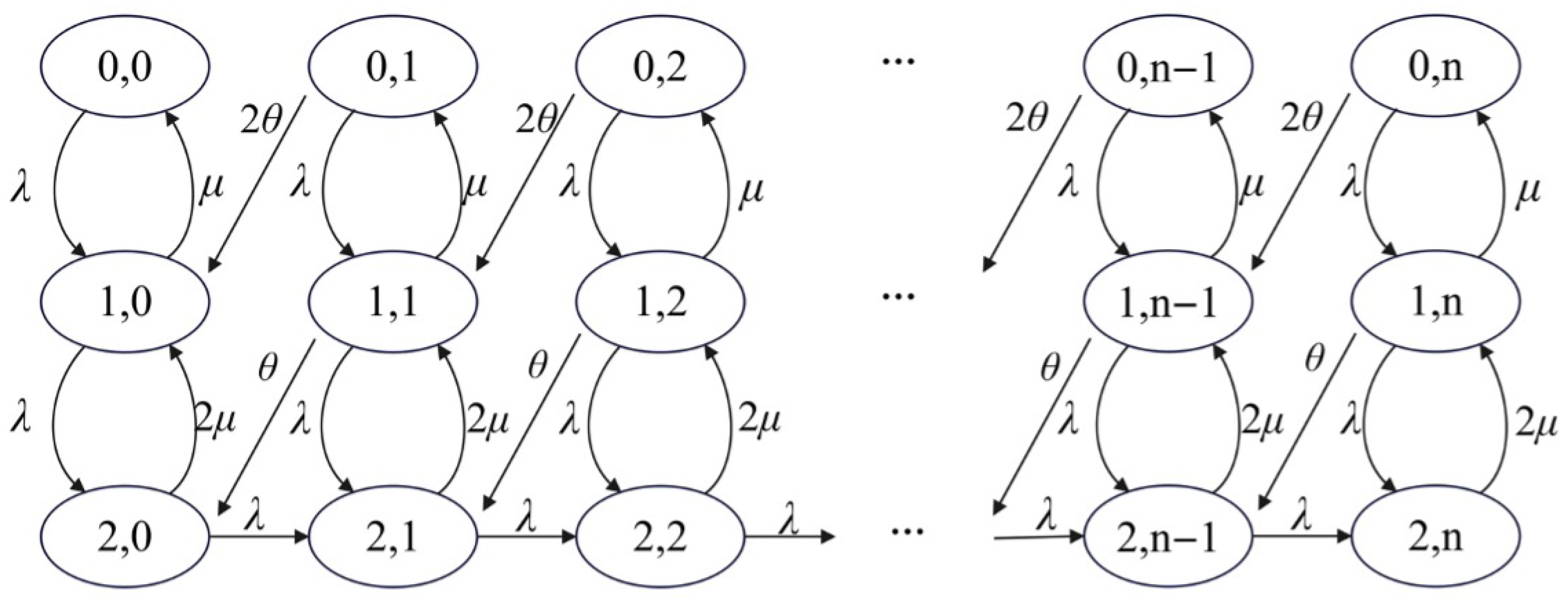
3.2. The Observable Case

Our analysis now centered on the observable case, where arriving customers can access real-time information concerning the exact number of customers waiting in an orbit. This additional information seems redundant for customers encountering idle servers, as they can be served immediately. Under the constant retrial policy, where customers in orbit are served on a first-come-first-served basis, those who find both servers occupied can leverage their precise orbital position knowledge to calculate their expected net benefit, making this information particularly valuable.

Analogous to the unobservable case, in the observable case, if arrivals find an idle server, they prefer to receive services at once. Therefore, our subsequent analysis concentrates on cases where both servers are occupied. In this observable case, customers employ a threshold-based retrial strategy: If a newly arriving customer observes that the number of customers in the retrial orbit is $n-1$ or fewer, they opt to join the orbit; otherwise, they balk. Correspondingly, the upper limit for the number of customers in orbit is n. Figure 2 presents the system transition diagram.

Given price P, in the observable case, we postulate that $n_e$ represents the equilibrium strategy adopted by customers. Under the assumption of Equation (1), it always has $n_e\ge 0$. We first examine the special case where $n_e=0$. If $R-P-cT(2,0)\le 0$, namely $P\ge R-{\displaystyle \frac{3c}{2\mu }}$, we have $n_e=0$. When $n_e>0$, the equilibrium strategy satisfies the following conditions:

$$\begin{array}{c}\hfill \left\{\begin{array}{c}R-P-cT(2,n_e)\ge 0,\hfill \\ R-P-cT(2,n_e+1)<0,\hfill \end{array}\right.\end{array}$$

where $T(2,n_e)={\displaystyle \frac{2\mu (\lambda +2\theta +\mu )+(\lambda +\theta )(\lambda +2\theta )}{2\theta \mu (\lambda +2\theta +2\mu )}}{n}_e+{\displaystyle \frac{3}{2\mu }}$. We obtain the threshold

$$\begin{array}{c}\hfill n_e=⌊\left({\displaystyle \frac{R-P}{c}}-{\displaystyle \frac{3}{2\mu }}\right){\displaystyle \frac{2\theta \mu (\lambda +2\theta +2\mu )}{2\mu (\lambda +2\theta +\mu )+(\lambda +\theta )(\lambda +2\theta )}}⌋.\end{array}$$

Before analyzing the optimal decision, we investigate the steady-state probability for a given threshold n.

Lemma 3. 

In the observable two-server constant retrial queue, if both servers are occupied, an arriving customer will opt to join the retrial orbit as long as the number of customers already waiting in orbit is $n-1$ or fewer. In other scenarios, customers enter without any restrictions. The steady-state probability $p_n(i,j)((i,j)\in \{0,1,2\}\times \{0,1,\cdots ,n\})$ is given by

$$\begin{array}{cc}\hfill & p_n(0,0)=\{{\lambda }^2+2\lambda \mu +2{\mu }^2\hfill \\ \hfill & +\left({\displaystyle \frac{1}{2\theta }}+{\displaystyle \frac{\epsilon }{\lambda }}\right)\left[(n+\epsilon -1){\lambda }^3+{\displaystyle \frac{\epsilon ({\lambda }^3-4\theta \mu (\lambda +\theta +\mu ))}{1-\epsilon }}\left(n-2-{\displaystyle \frac{{\epsilon }^2-{\epsilon }^n}{1-\epsilon }}\right)\right]{\}}^{-1},\hfill \\ \hfill & p_n(1,0)={\displaystyle \frac{\lambda }{\mu }}{p}_n(0,0),\hfill \\ \hfill & p_n(2,0)={\displaystyle \frac{{\lambda }^2(\lambda +2\theta +2\mu )}{4{\mu }^2(\lambda +\theta +\mu )}}{p}_n(0,0),\hfill \end{array}$$

$$\begin{array}{cc}\hfill & p_n(0,j)={\displaystyle \frac{p_n(0,0)}{4\theta \mu (\lambda +\theta +\mu )}}\left\{{\lambda }^3+\left[{\lambda }^3-4\theta \mu (\lambda +\theta +\mu )\right]{\displaystyle \frac{\epsilon -{\epsilon }^j}{1-\epsilon }}\right\},j=1,2,\cdots ,n-1,\hfill \\ \hfill & p_n(1,j)={\displaystyle \frac{\lambda +2\theta }{\mu }}{p}_n(0,j),j=1,2,\cdots ,n,\hfill \\ \hfill & p_n(2,j)={\displaystyle \frac{(\lambda +\theta +\mu )(\lambda +2\theta )-\lambda \mu }{2{\mu }^2}}{p}_n(0,j)-{\displaystyle \frac{\theta }{\mu }}{p}_n(0,j+1),j=1,2,\cdots ,n-1,\hfill \\ \hfill & p_n(0,n)=\epsilon p_n(0,n-1),\hfill \\ \hfill & p_n(2,n)={\displaystyle \frac{\epsilon \left[\right(\lambda +\theta \left)\right(\lambda +2\theta )+2\theta \mu ]}{2{\mu }^2}}{p}_n(0,n),\hfill \end{array}$$

where $\epsilon ={\displaystyle \frac{\lambda (\lambda +\theta +\mu )(\lambda +2\theta )-{\lambda }^2\mu }{4\theta \mu (\lambda +\theta +\mu )}}$.

3.2.1. Profit-Maximizing Price in the Observable Case

Given customers’ equilibrium threshold $n_e\left(P\right)$, similar to Section 3.1.1, profit-maximising manager aims to find an optimal price to maximize the profit, as shown below.

$$\begin{array}{c}\hfill {\Pi }_o\left(P\right)=\lambda (1-p_{n_e\left(P\right)}(2,n_e\left(P\right)))P.\end{array}$$

(6)

If the price $P\ge R-{\displaystyle \frac{3c}{2\mu }}$, then $n_e\left(P\right)=0$. In this case, the profit function becomes

$$\begin{array}{c}\hfill {\Pi }_o\left(P\right)=\lambda \left(1-{\displaystyle \frac{{\lambda }^2}{{\lambda }^2+2\lambda \mu +2{\mu }^2}}\right)P={\displaystyle \frac{2\lambda \mu (\lambda +\mu )}{{\lambda }^2+2\lambda \mu +2{\mu }^2}}P.\end{array}$$

(7)

Equation (7) is the same as Equation (4); hence, the optimal price is still $P^m$.

If the price $P<R-{\displaystyle \frac{3c}{2\mu }}$, the threshed satisfies $n_e\left(P\right)>0$. We denote the optimal price of this case by $P_o^{*}$ if it exists. In summary, the optimal price $P_o$ is either $P^m$ or $P_o^{*}$.

3.2.2. Welfare-Maximizing Price in the Observable Case

In the observable scenario, the social welfare function can be formulated as follows:

$$\begin{array}{cc}\hfill {SW}_o\left(n\right)=& \left[\sum _{j=0}^n{p}_n(0,j)+\sum _{j=0}^n{p}_n(1,j)\right]\left(R-{\displaystyle \frac{c}{\mu }}\right)+\sum _{j=0}^{n-1}{p}_n(2,j)(R-cT(2,j+1)).\hfill \end{array}$$

Arranging it, this function becomes

$$\begin{array}{cc}\hfill {SW}_o\left(n\right)=& \lambda \left(1-p_n(2,n)\right)\left(R-{\displaystyle \frac{c}{\mu }}\right)\hfill \\ \hfill & -c\lambda \sum _{j=0}^{n-1}{p}_n(2,j)\left({\displaystyle \frac{1}{2\mu }}+(j+1){\displaystyle \frac{2\mu (\lambda +2\theta +\mu )+(\lambda +\theta )(\lambda +2\theta )}{2\theta \mu (\lambda +2\theta +2\mu )}}\right).\hfill \end{array}$$

(8)

The socially optimal threshold $n_{sw}$ is an integer, and it must satisfy the following inequality:

$$\begin{array}{c}\hfill \left\{\begin{array}{c}S{W}_o\left(n_{sw}\right)\ge S{W}_o(n_{sw}-1),\hfill \\ S{W}_o\left(n_{sw}\right)\ge S{W}_o(n_{sw}+1).\hfill \end{array}\right.\end{array}$$

In the observable case, let $P_o^{sw}$ be the socially optimal price if it exists. Then, $P_o^{sw}=R-cT(2,n_{sw})$ if the social threshold is $n_{sw}$. Due to the complexity of $S{W}_o\left(n\right)$, deriving its analytic solution $n_{sw}$ for the general case appears to be extremely challenging. Consequently, obtaining a theoretical result for $P_o^{sw}$ is tough. Hence, we ultimately resort to finding it via numerical examples.

4. Numerical Results

A numerical analysis is performed in this section to provide some managerial insights.

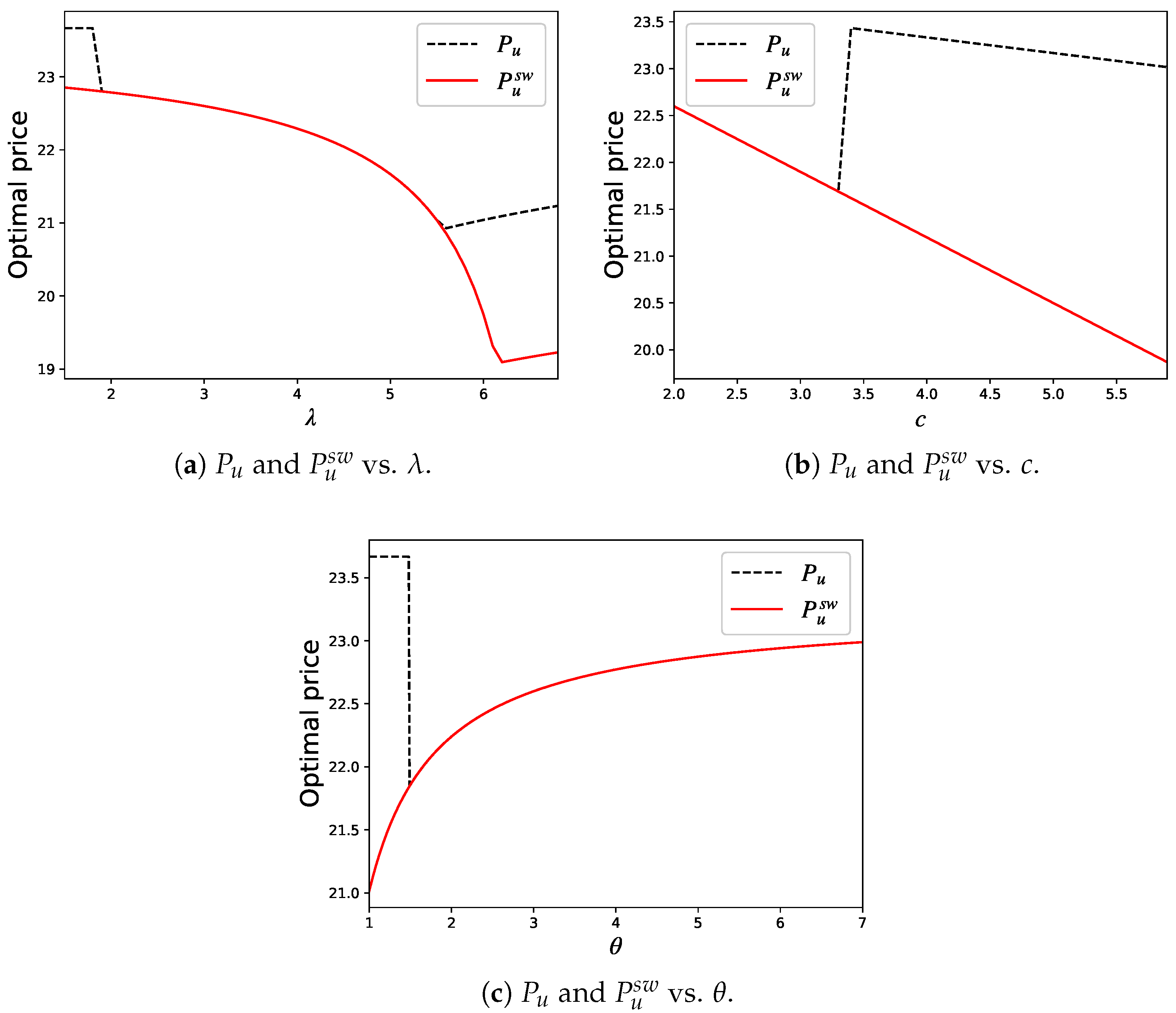
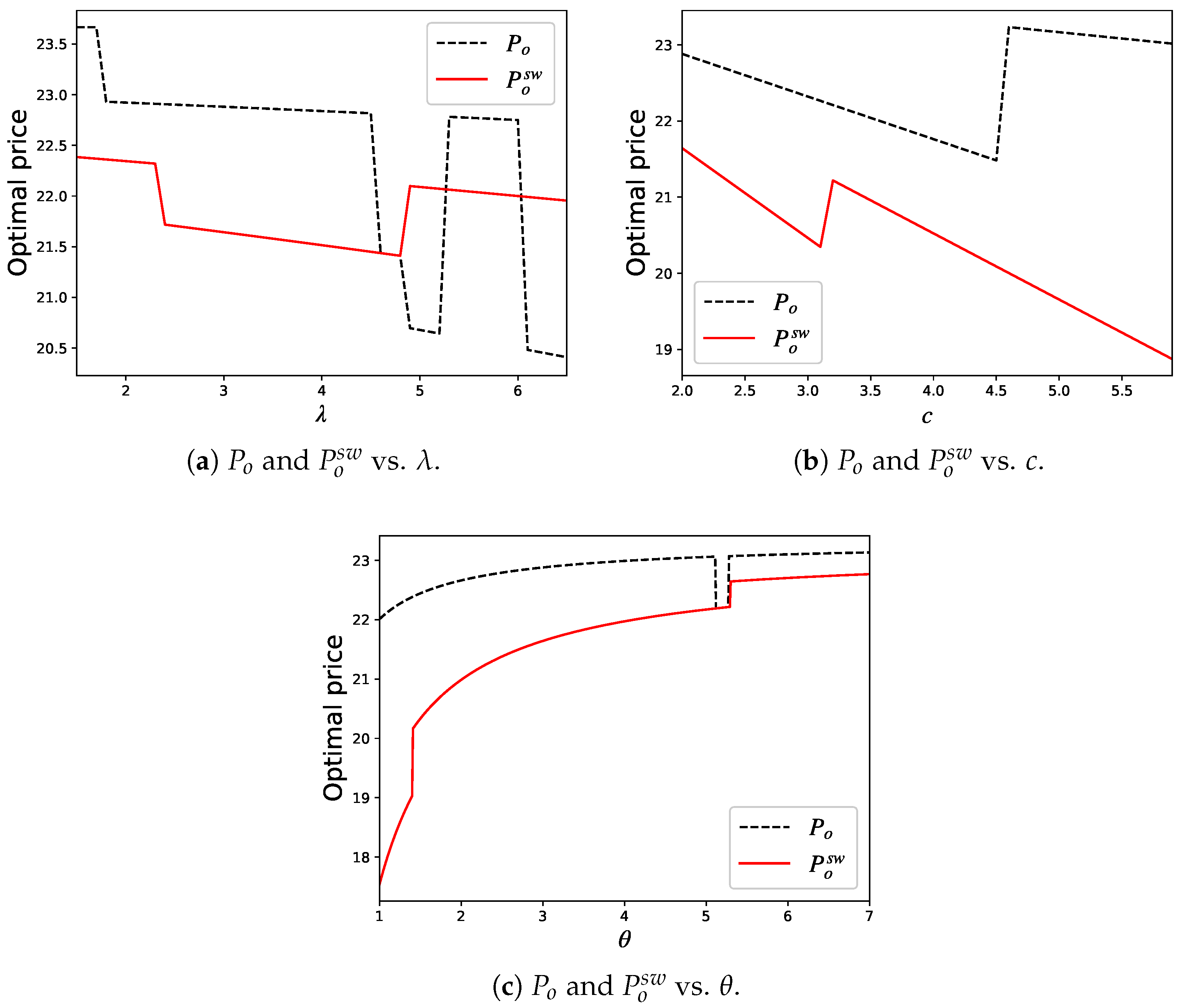
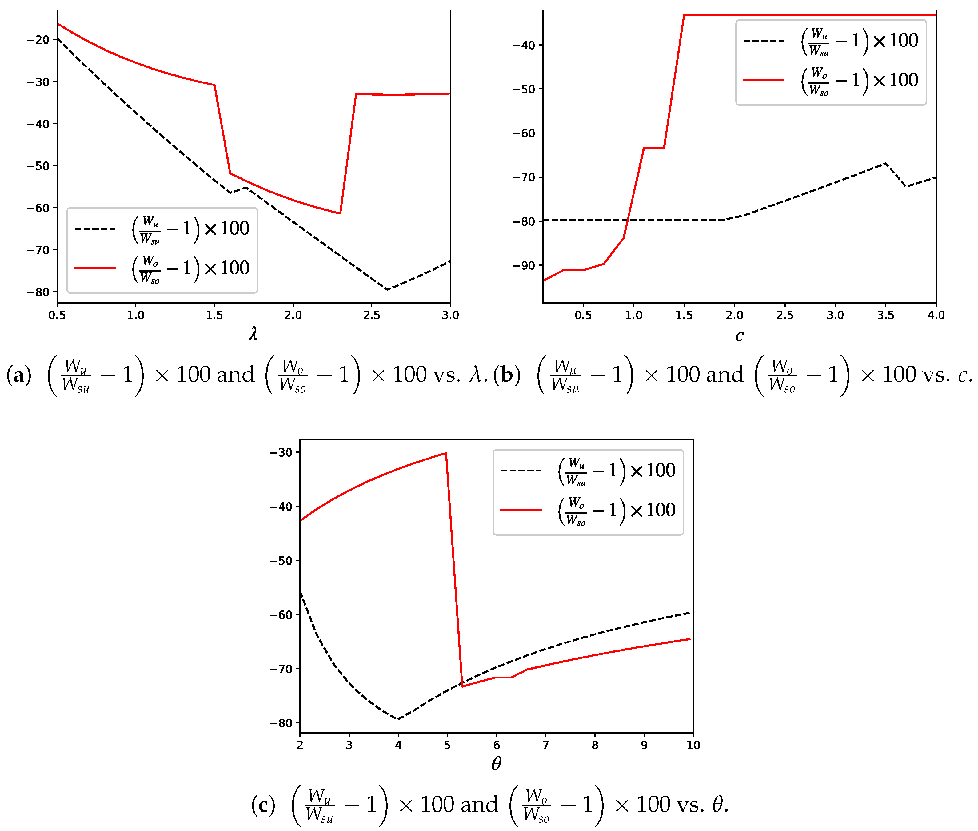
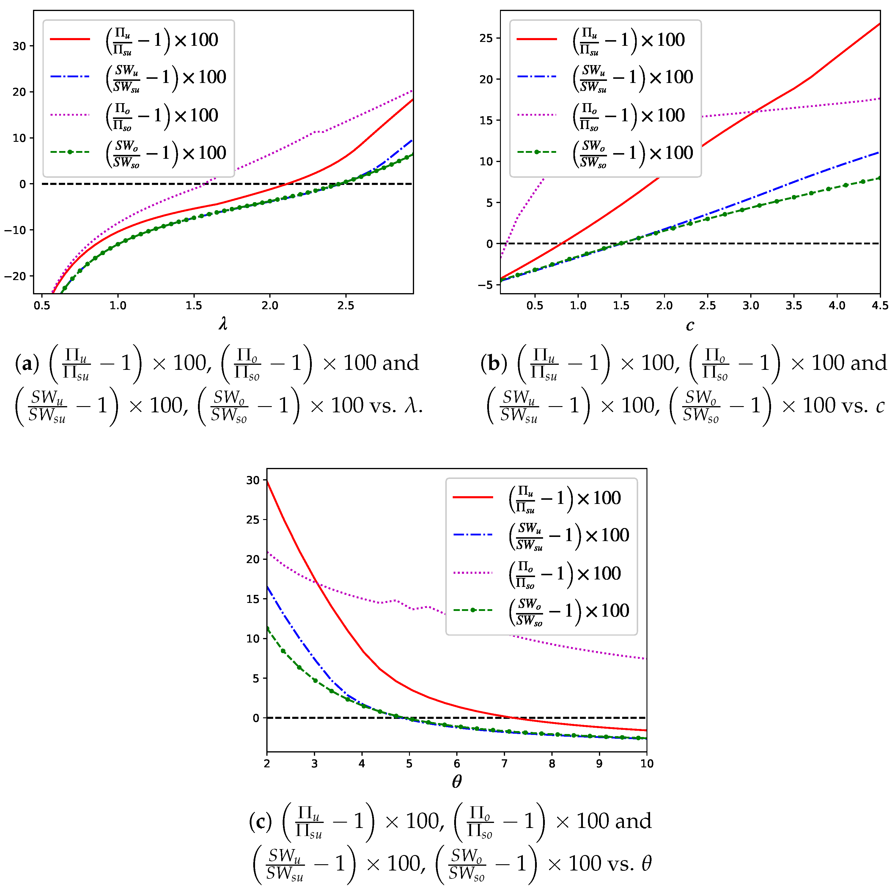
4.1. Sensitivity Analysis

This subsection explores the effect of the system utilization factor ${\displaystyle \frac{\lambda }{\mu }}$, the reward-to-cost ratio ${\displaystyle \frac{R}{\theta }}$, and the retrial rate $\theta$ of the optimal price, including the profit-maximizing price ($P_u$, $P_o$) and welfare-maximizing price ($P_u^{sw}$, $P_o^{sw}$). For brevity, in the first two sub-cases, we normalize $\mu =6$ and $R=24$. Unless otherwise specified, other parameters’ values are given as follows: $c=2$, $\lambda =3$, $\theta =3$.

From Figure 3, we observe that the profit-maximizing price consistently equals or exceeds the welfare-maximizing price. When the parameters fall within specific ranges, such as $\lambda \in [1.89, 5.50]$, $c\in [2.0, 3.2]$ and $\theta \in [1.5, 7.0]$, they are the same. In these situations, retrial customers obtain zero utility, no matter the profit or welfare maximization perspective. However, beyond these parameter ranges, the social planner strategically maintains positive utility to attract and retain customers. We notice that when the parameters change, profit-maximising manager and the social planner may adopt the same strategy to control prices. For example, when $\lambda$ increases, congestion in the orbit is increased, leading customers to be hesitant about joining. Consequently, the two maximisers reduce their prices to attract customers. However, when $\lambda$ is sufficiently large, they will increase the price to avoid the orbit from becoming more congested. In contrast, their strategies might also be different. When customers become impatient (i.e., c increases), the profit-maximising managers initially opt to lower prices, followed by a sharp increase, and then a subsequent decrease. In contrast, the social planner reduces prices, intending to retain a larger customer base. When the retrial rate $\theta$ changes, we observe that their strategies are different. This can be understood intuitively as follows: the social planner is inclined to provide positive utility to customers, whereas profit-maximizing managers do not have this inclination. These findings highlight the complex interplay between system parameters and decision-making objectives in pricing strategy formulations, particularly in balancing congestion management with customer behavior considerations.

When comparing Figure 3 to Figure 4, the availability of information considerably influences the pricing strategies adopted by the profit maximizer and the social planner. In scenarios where customers can access real-time queue length information in the orbit (i.e., the observable case), their behavior tends to become more rational, necessitating that both decision makers adjust their pricing strategies in response to this heightened level of customer rationality. These changes lead to distinct pricing strategies that differ from those in the unobservable case.

4.2. Comparative Analysis

This subsection examines the alterations in customers’ sojourn time, profit, and social welfare when the retrial queue comprises two servers, as compared to the corresponding outcomes in a single-server system. To facilitate this comparison, we incorporate the unit service capacity $\kappa$ in the objective function. Unless otherwise defined, the parameter values utilized in the analysis are $R=25$, $c=2$, $\lambda =2.6$, $\mu =6$, $\theta =4$, and $\kappa =0.5$.

(i) In the context of a single-server constant retrial queue (Economou and Kanta [8]), the expected sojourn times for a customer in both the unobservable and observable cases are given, respectively, by

$$\begin{array}{cc}\hfill & W_{su}=p_0{\mid }_{q=q_{se}}·{\displaystyle \frac{1}{\mu }}+p_1{\mid }_{q=q_{se}}·\left[{\displaystyle \frac{\lambda +\theta +\mu }{\mu \theta -q_{se}\lambda (\lambda +\theta )}}+{\displaystyle \frac{1}{\mu }}\right],\hfill \\ \hfill & W_{so}=\sum _{j=0}^{n_{se}+1}{p}_{0,j}·{\displaystyle \frac{1}{\mu }}+\sum _{j=0}^{n_{se}}{p}_{1,j}·\left[{\displaystyle \frac{\lambda +\theta +\mu }{\mu \theta }}(j+1)+{\displaystyle \frac{1}{\mu }}\right],\hfill \end{array}$$

where $p_i$ and $p_{i,j}$ can be found in Propositions 3.1 and 4.2. $q_{se}$ and $n_{se}$ are the customers’ equilibrium strategies, as outlined in Theorems 3.1 and 4.1. In our system, we compute the expected sojourn times for a customer for both the unobservable and observable cases, as outlined below.

$$\begin{array}{cc}\hfill & W_u=(p_0\left(1\right){\mid }_{q=q_e}+p_1\left(1\right){\mid }_{q=q_e})·{\displaystyle \frac{1}{\mu }}+q_e{p}_2\left(1\right){\mid }_{q=q_e}·W_u\left(q_e\right),\hfill \\ \hfill & W_o=\left(\sum _{j=0}^{n_e}{p}_{n_e}(0,j)+\sum _{j=0}^{n_e}{p}_{n_e}(1,j)\right)·{\displaystyle \frac{1}{\mu }}+\sum _{j=0}^{n_e-1}{p}_{n_e}(2,j)·T(2,j+1).\hfill \end{array}$$

Let $\left({\displaystyle \frac{W_u}{W_{su}}}-1\right)\times 100$ and $\left({\displaystyle \frac{W_o}{W_{so}}}-1\right)\times 100$ correspond to the percentage change measure in customers’ sojourn time of the unobservable and observable cases.

By examining Figure 5, we find that $\left({\displaystyle \frac{W_u}{W_{su}}}-1\right)\times 100<0$ and $\left({\displaystyle \frac{W_o}{W_{so}}}-1\right)\times 100<0$ as $\lambda$, c and $\theta$ vary. Sometimes, this measure increases up to 90%. This implies that, as expected, increasing the number of servers could relieve system congestion. Notably, most of the time, $\left({\displaystyle \frac{W_u}{W_{su}}}-1\right)\times 100$ is less than $\left({\displaystyle \frac{W_o}{W_{so}}}-1\right)\times 100$, which indicates that, compared to the observable case, the reduction in customers’ sojourn time is more obvious in the unobservable case. An explanation for this surprising result could be that in a two-server system, which is less congested, customers perhaps adjust their expectations and behavior based on their observations of the system state, behaving more rationally. However, if the queue length is unobservable, customers do not have the same level of information that can be used to influence their behavior.

(ii) We now present some findings related to profit and social welfare. Based on the work of Armony et al. [29], for both unobservable and observable scenarios, the profit functions outlined in Economou and Kanta [8] can be modified as follows:

$$\begin{array}{c}\hfill {\Pi }_{su}\left(P\right)={\displaystyle \frac{\lambda \mu }{\mu +\lambda (1-q_{se})}}P-\kappa \mu ,{\Pi }_{so}\left(P\right)={\lambda }^{*}\left(n_{se}\right)P-\kappa \mu ,\end{array}$$

where ${\lambda }^{*}\left(n\right)=\lambda -\theta {\rho }^{n+1}{\left({\displaystyle \frac{\theta \mu }{{\lambda }^2}}+{\displaystyle \sum _{i=0}^n}{\rho }^i+{\displaystyle \frac{\theta }{\lambda }}{\displaystyle \sum _{i=0}^{n+1}}{\rho }^i\right)}^{-1}$ and $\rho ={\displaystyle \frac{\lambda (\lambda +\theta )}{\mu \theta }}$. The social welfare functions of the two cases are, respectively,

$$\begin{array}{cc}\hfill S{W}_{su}\left(q\right)=& {\displaystyle \frac{(\lambda R+c)\mu }{\mu +\lambda (1-q)}}-{\displaystyle \frac{c\mu \theta }{\mu \theta -\lambda q(\lambda +\theta )}}-\kappa \mu ,\hfill \\ \hfill S{W}_{so}\left(n\right)=& {\lambda }^{*}\left(n\right)\left(R-{\displaystyle \frac{c}{\mu }}\right)-{\displaystyle \frac{\lambda c(\lambda +\theta +\mu )}{\mu \theta }}\sum _{j=0}^n(j+1)p_{1,j}-\kappa \mu .\hfill \end{array}$$

In our system, Equations (3) and (6) subtract $2\kappa \mu$, which are the profit functions of unobservable and observable cases when considering the service capacity costs. Equations (5) and (8) subtract $2\kappa \mu$, which are the social welfare functions of the two cases, when considering the service capacity costs. For the analysis, we define $\left({\displaystyle \frac{{\Pi }_u}{{\Pi }_{su}}}-1\right)\times 100$, $\left({\displaystyle \frac{{\Pi }_o}{{\Pi }_{so}}}-1\right)\times 100$ and $\left({\displaystyle \frac{S{W}_u}{S{W}_{su}}}-1\right)\times 100$, $\left({\displaystyle \frac{S{W}_o}{S{W}_{so}}}-1\right)\times 100$ as corresponding to the percentage change in profit and social welfare of the unobservable and observable cases, respectively (Figure 6).

An intriguing finding from each of these figures is that $\left({\displaystyle \frac{{\Pi }_u}{{\Pi }_{su}}}-1\right)\times 100>\left({\displaystyle \frac{S{W}_u}{S{W}_{su}}}-1\right)\times 100$ and $\left({\displaystyle \frac{{\Pi }_o}{{\Pi }_{so}}}-1\right)\times 100>\left({\displaystyle \frac{S{W}_o}{S{W}_{so}}}-1\right)\times 100$. This suggests that the manager aiming to maximize profits has a stronger incentive to deploy additional servers compared to the social planner.

5. Conclusions

This study delves into pricing decisions in a retrial queue comprising two servers. Under the unobservable and observable cases, we first investigate retrial customers’ sojourn time. Based on this, we examine their equilibrium strategies and find that different prices will lead to different retrial behaviors. Also, we analyze profit and welfare maximization prices, revealing that they may differ even in the unobservable scenario. Compared with the single-server queue, the reduction in expected sojourn times is more obvious in the unobservable case. Moreover, when the market size is substantial, customers are less willing to wait. Additionally, when the retrial rate is low, the two-server system outperforms the single-server system in terms of both profit and social welfare. The manager who seeks to maximize profits has a stronger incentive to arrange multiple servers than the social planner.

References

1. Lai, C.; Kasim, E.; Muhammadhaji, A. Dynamic Analysis of a Standby System with Retrial Strategies and Multiple Working Vacations. Mathematics 2024, 12, 3999. [Google Scholar] [CrossRef]
2. Samanta, S.K.; Rashmi, K.M. Analytical and computational aspects of a batch arrival retrial queue with a constant retrial policy. In Quality Technology & Quantitative Management; Taylor & Francis: Abingdon-on-Thames, UK, 2025; pp. 1–28. [Google Scholar]
3. Aissani, A. An MX/G/1 energetic retrial queue with vacations and control. IMA J. Manag. Math. 2011, 21, 13–32. [Google Scholar] [CrossRef]
4. Tapiero, C.S. Energy consumption and environmental pollution: A stochastic model. IMA J. Manag. Math. 2009, 20, 263–273. [Google Scholar] [CrossRef]
5. Dimitriou, I. A single server retrial queue with event-dependent arrival rates. Ann. Oper. Res. 2023, 331, 1053–1088. [Google Scholar] [CrossRef]
6. Artalejo, J.R.; Gómez-Corral, A. Retrial Queueing Systems: A Computational Approach; Springer: Berlin/Heidelberg, Germany, 2008. [Google Scholar]
7. Falin, G.; Templeton, J.G. Retrial Queues; CRC Press: Boca Raton, FL, USA, 1977. [Google Scholar]
8. Economou, A.; Kanta, S. Equilibrium customer strategies and social–profit maximization in the single-server constant retrial queue. Nav. Res. Log. 2011, 58, 107–122. [Google Scholar] [CrossRef]
9. Cui, S.; Su, X.; Veeraraghavan, S. A model of rational retrials in queues. Oper. Res. 2019, 67, 1699–1718. [Google Scholar] [CrossRef]
10. Armony, M.; Maglaras, C. Contact centers with a call-back option and real-time delay information. Oper. Res. 2004, 52, 527–545. [Google Scholar] [CrossRef]
11. Tang, Y.; Guo, P.; Wang, Y. Equilibrium queueing strategies of two types of customers in a two-server queue. Oper. Res. Lett. 2018, 46, 99–102. [Google Scholar] [CrossRef]
12. Naor, P. The regulation of queue size by levying tolls. Econometrica 1969, 37, 15–24. [Google Scholar] [CrossRef]
13. Edelson, N.M.; Hilderbrand, D.K. Congestion tolls for Poisson queuing processes. Econometrica 1975, 43, 81–92. [Google Scholar] [CrossRef]
14. Hassin, R.; Haviv, M. To Queue or Not to Queue: Equilibrium Behavior in Queueing Systems; Springer Science and Business Media: Berlin, Germany, 2003. [Google Scholar]
15. Hassin, R. Rational Queueing; CRC Press: Boca Raton, FL, USA, 2016. [Google Scholar]
16. Hassin, R.; Haviv, M. Equilibrium strategies and the value of information in a two line queueing system with threshold jockeying. Stoch. Model. 1994, 10, 415–435. [Google Scholar] [CrossRef]
17. Hassin, R. On the advantage of being the first server. Manage. Sci. 1996, 42, 618–623. [Google Scholar] [CrossRef]
18. Zhao, C.; Wang, Z. The impact of line-sitting on a two-server queueing system. Eur. J. Oper. Res. 2023, 74, 748–761. [Google Scholar] [CrossRef]
19. Zhou, W.; Huang, W.; Hsu, V.N.; Guo, P. On the benefit of privatization in a mixed duopoly service system. Manag. Sci. 2023, 69, 1486–1499. [Google Scholar] [CrossRef]
20. Cattani, K.; Schmidt, G.M. The pooling principle. Informs Trans. Edu. 2005, 5, 17–24. [Google Scholar] [CrossRef]
21. Yechiali. Customers’ optimal joining rules for the GI/M/s queue. Manag. Sci. 1972, 18, 434–443. [Google Scholar]
22. Wang, J.; Zhang, Y.; Zhang, Z.G. Strategic joining in an M/M/K queue with asynchronous and synchronous multiple vacations. J. Oper. Res. Soc. 2021, 72, 161–179. [Google Scholar] [CrossRef]
23. Kulkarni, V.G. On queueing systems by retrials. J. Appl. Probab. 1983, 20, 380–389. [Google Scholar] [CrossRef]
24. Elcan, A. Optimal customer return rate for an M/M/1 queueing system with retrials. Probab. Eng. Inform. Sci. 1994, 8, 521–539. [Google Scholar] [CrossRef]
25. Hassin, R.; Haviv, M. On optimal and equilibrium retrial rates in a queueing system. Probab. Eng. Inform. Sci. 1994, 10, 223–227. [Google Scholar] [CrossRef]
26. Wang, J.; Zhang, F. Strategic joining in M/M/1 retrial queues. Eur. J. Oper. Res. 2013, 230, 76–87. [Google Scholar] [CrossRef]
27. Wang, Z.; Wang, J. Information heterogeneity in a retrial queue: Throughput and social welfare maximization. Queueing Syst. 2019, 92, 131–172. [Google Scholar] [CrossRef]
28. Zhang, Y.; Wang, J. Managing retrial queueing systems with boundedly rational customers. J. Oper. Res. Soc. 2023, 74, 748–761. [Google Scholar] [CrossRef]
29. Armony, M.; Plambeck, E.; Seshadri, S. Sensitivity of optimal capacity to customer impatience in an unobservable M/M/S queue (Why you shouldn’t shout at the DMV). Manuf. Serv. Oper. Manag. 2009, 11, 19–32. [Google Scholar] [CrossRef]
30. Hanukov, G. Improving efficiency of service systems by performing a part of the service without the customer’s presence. Eur. J. Oper. Res. 2022, 302, 606–620. [Google Scholar] [CrossRef]
31. Neuts, M.F. Matrix-Geometric Solutions in Stochastic Models: An Algorithmic Approach; Courier Corporation: Chelmsford, MA, USA, 1994. [Google Scholar]
Figure 1. Transition diagram for the unobservable scenario.
Mathematics 13 01310 g001
Figure 2. Transition diagram of the observable scenario.
Mathematics 13 01310 g002
Figure 3. The optimal prices versus different parameters in the observable case.
Mathematics 13 01310 g003
Figure 4. The optimal prices versus different parameters in the observable case.
Mathematics 13 01310 g004
Figure 5. Two measures, W u W s u 1 × 100 and W o W s o 1 × 100 versus λ , c and θ , respectively.
Mathematics 13 01310 g005
Figure 6. Π u Π s u 1 × 100 , Π o Π s o 1 × 100 and S W u S W s u 1 × 100 , S W o S W s o 1 × 100 vs. λ , c and θ , respectively.
Mathematics 13 01310 g006
Disclaimer/Publisher’s Note: The statements, opinions and data contained in all publications are solely those of the individual author(s) and contributor(s) and not of MDPI and/or the editor(s). MDPI and/or the editor(s) disclaim responsibility for any injury to people or property resulting from any ideas, methods, instructions or products referred to in the content.