Application of Integrable Systems in Carbon Price Determination

Abstract

This paper examines carbon emission allowances and pricing mechanisms in the context of climate change, utilizing nonlinear evolution equation theory. Through empirical analysis of European Union EUA option data using the EGARCH model, the study identifies non-normal distribution characteristics in carbon market returns and explores how policy innovations influence price fluctuations. A key contribution is its application of soliton theory to analyze carbon price dynamics. By employing integrable systems like the (1 + 1)-dimensional Boussinesq equation, it aims to develop a mathematical model for carbon price stability. The research calculates the Lax pair for this system and uses Hirota’s bilinear method among other techniques to investigate whether carbon prices can exhibit soliton phenomena with consistent waveforms and amplitudes. This work provides insights into the carbon market’s dynamics and lays a theoretical foundation for better simulation, market behavior prediction, and optimization of climate policies.

1. Introduction

The increasing urgency of the global climate change issue has brought it to the forefront of international attention. A widespread scientific consensus points to human activities as the primary driver of climate change, manifested through the release of large amounts of greenhouse gases from fossil fuel combustion, pollution emitted during industrial production processes, and the depletion of carbon sinks due to extensive deforestation. Among these factors, the rise in carbon dioxide emissions stands out as a key driver of climate change. In response to this challenge, the international community has actively implemented a series of measures over the past few decades. This includes the signing of the United Nations Framework Convention on Climate Change (UNFCCC) and the adoption of landmark international legal instruments like the Kyoto Protocol and the Paris Agreement [1]. These agreements aim to limit the total global greenhouse gas emissions and strive to mitigate and adapt to the adverse impacts of climate change. Within the strategies to address climate change, the carbon emission rights system and carbon pricing mechanisms have increasingly played a pivotal role. Governments and international organizations establish carbon emission rights through laws, regulations, and policies to effectively manage and allocate emission quotas [2]. Enterprises and institutions operate within these quotas, trading carbon emission rights in the market. If actual emissions exceed the quota, additional allowances must be purchased. Conversely, if successful emission reductions result in emissions below the quota, the remaining allowances can be sold. The operation of the carbon emission trading market internalizes the cost of carbon emissions into production costs, effectively incentivizing businesses to adopt more environmentally friendly and energy-efficient practices in their production and operations. Additionally, carbon pricing, determined by governments or international organizations through taxation policies and emissions trading, reflects the actual environmental damage caused by carbon emissions and encourages businesses and individuals to take proactive measures to reduce emissions.

Since the late 19th century, nonlinear evolutionary equations (NLEEs) have emerged as a powerful theoretical tool, playing a crucial role in describing wave propagation phenomena in mixtures of liquids and gases. These complex mathematical models not only play a key role in revealing the essential features of nonlinear physical phenomena but also find extensive applications in various fields of engineering and basic science, such as fluid mechanics, acoustics, and even financial economics [3]. Particularly, research utilizing the Boussinesq equation and its related extended models [4] has allowed scholars to delve deeper into the intrinsic laws governing wave propagation in weakly nonlinear and weakly dispersive media. For many years, the research on nonlinear evolutionary equations has attracted the attention of many scientists, with a continuous stream of research outcomes demonstrating significant influence in the field. These outcomes encompass advancements in solution methods and the analysis of the integrability of equation systems. The introduction of mathematical principles and techniques, such as Lax pairs [5], Bäcklund transformations [6], and infinite conservation laws [7], has laid a solid foundation for determining and proving the integrability of systems. The study of soliton theory not only creates a new discipline in mathematical physics but also has applications in high-tech fields such as biosystems engineering [8,9], agriculture [10,11], and food chemistry [12,13].

Despite this, research exploring the interaction between carbon emission rights and carbon prices using integrable system theory remains insufficient. This paper aims to fill this gap by investigating the potential value of integrable systems in determining carbon prices [14]. By leveraging these mathematical models, the study seeks to provide a solid theoretical foundation and innovative policy recommendations to strengthen global climate governance mechanisms, promote the transformation of low-carbon economies, and contribute to achieving the United Nations Sustainable Development Goals. By integrating advanced mathematical theories with real-world economic practices, this research holds promise for opening up a new path to help the international community manage carbon emissions more scientifically and effectively, mitigate climate change, and foster the transition towards a sustainable global economy.

2. Sample Selection and Data Analysis

Considering the complexity and nonlinear characteristics of carbon emission-rights price volatility, this chapter selects the EGARCH model [15] for forecast analysis. The EGARCH model [16], i.e., exponential GARCH model, is an extension of the generalized autoregressive conditional heteroskedasticity model (GARCH model), which can better capture the asymmetry and leverage effect of time-series data. In the carbon emission-rights market, price fluctuations often exhibit asymmetric characteristics due to the psychological expectations of market participants, policy adjustments, and other factors, so the EGARCH model has a significant advantage in this type of research.

2.1. Sample Selection

Currently, China has not initiated carbon emission allowance option trading, and thus relevant data in this domain do not exist. The European Union Allowance Option (EUA Option) is the most prominent carbon emission rights option internationally, and it is considered the best research subject in terms of trading history and market turnover. Therefore, this paper selects the EUA Option as the sample for empirical research. To ensure the timeliness of the data, this paper chooses the carbon emission allowance option contract expiring on 13 December 2023 by the Intercontinental Exchange (ICE), named the Dec23 Option, as the research object. The option type is a put option with an exercise price of EUR 100. Correspondingly, its underlying asset is the carbon emission futures contract expiring on 18 December 2023, named the Dec23 Future. The closing price unit is in euros per ton of carbon dioxide equivalent.

To enhance the generalizability of the results, this paper selects historical data from the 18 months leading up to a certain day (inclusive of that day) to analyze the closing prices of carbon emission allowance options for the 10 trading days following that day. Consequently, the chosen data for options and futures spans from 1 August 2021 to 28 February 2023.

To make the model comparison results more credible, this paper has created two datasets from the closing prices of options and futures: Data1 and Data2. Data1 spans from 1 August 2021 to 14 February 2023, comprising 399 data points, while Data2 covers from 15 August 2021 to 28 February 2023, also with 399 data points. For Data1, the period from 1 August 2021 to 31 January 2023 is designated as the training set, and the period from 1 February 2023 to 14 February 2023 is used as the test set. The same approach is applied to Data2.

Additionally, for the sake of clarity in describing the data, this paper primarily focuses on the detailed description of Data1 while only presenting the results of Data2 briefly.

2.2. Carbon Emission Rights Futures Data Processing

Since the calculation of volatility and the Hurst exponent [17] are based on returns, it is necessary to process the closing price data of carbon emission futures to obtain a sequence of returns. This paper will adopt the following processing method: firstly, the natural logarithm of the daily closing price data will be taken, and then the data will be differenced to obtain the log returns, denoted as:

$$y_i=lni-ln(i-1).$$

(1)

where i represents an index in a time series, indicating different points in time.

2.2.1. Descriptive Statistical Analysis of Yield Series

Descriptive statistics analysis of the yield series obtained from Data1 yielded the following results (Figure 1):

From Figure 1, it can be observed that the returns of the futures contract closing prices do not follow a normal distribution. Moreover, the kernel density curve exhibits higher kurtosis and thicker tails compared to the normal density curve.

Moreover, the Kolmogorov–Smirnov test (K-S test) [18] was employed to quantitatively assess the non-normality of the return rate series. By comparing the sample cumulative distribution function (CDF) with that of the theoretical normal distribution, we calculated the maximum deviation D:

$$D=\underset{x}{sup}|F_n\left(x\right)-F\left(x\right)|,$$

(2)

where $F_n\left(x\right)$ is the empirical distribution function of the sample and $F\left(x\right)$ is the standard normal distribution function. Null hypothesis $H_0$ is that the data follow a normal distribution and the significance level is set as $\alpha =0.05$.

After verification, the K-S statistic $D=0.121>{\displaystyle \frac{1.36}{\sqrt{n}}}={\displaystyle \frac{1.36}{\sqrt{399}}}\approx 0.068$ and probability value $p<0.001$ provide strong evidence against the null hypothesis. This finding aligns with the pronounced peak and thick tail characteristics observed in the kernel density curve presented in Figure 1, further confirming that the yield of carbon futures exhibits a nonlinear fluctuation pattern that significantly deviates from a normal distribution.

2.2.2. Return to Baseline

The test of the innovativeness of carbon emission trading and investment policies is as follows (

Table 1. Innovative tests of carbon emission trading and investment policies.

Variant	−1	−2
	Innovation	Innovation
Region × Post	0.045 ***	-
	−0.017
Region × Year2021	-	0.005
		−0.023
Region × Year2022	-	0.001
		−0.024
Region × Year2023	-	0.048 ***
		−0.022
Control variable	Yes	Yes
Year fixed	Yes	Yes
City × industry fixed	Yes	Yes
Constant term (math.)	−4.217 ***	−4.158 ***
	−0.377	−0.38
Sample size	144,936	144,936
R2	0.897	0.897

*** indicates significance at the $1\%$ level.

). In Table 1, “−1” represents a model that incorporates solely the “Region × Post” variable, utilized to evaluate the overall impact of policy innovation on carbon price volatility. Conversely, “−2” includes additional interaction terms such as “Region × Year2021”, “Region × Year2022”, and “Region × Year2023”, which are employed to analyze the specific effects of policy innovation on carbon price volatility across different years. The comparison between these two variants reveals significant disparities in policy impacts across various time points and regions, thereby offering a more comprehensive understanding of the dynamic effects engendered by policy innovation.

Before modeling the return series, it is necessary to extract level information through techniques such as ARIMA modeling [19], which requires a benchmark regression to be performed on the returns. Additionally, the methods for regression testing include time series plots, unit root tests, and PP tests [20]. Since the unit root test assumes that the series satisfies homoscedasticity, whereas the PP test does not impose this constraint, the PP test is ultimately chosen for use.

2.2.3. Conduction Mechanism Test

The analysis of the transmission mechanism in the time series is closely related to the level modeling of the time series. We use an R language program to analyze the transmission mechanism of the return series, as indicated in the table below (see

Table 2. Conduction mechanism test.

Variant	(1)	(2)	Variant	(3)	Variant	(4)
	Inn. 1	Inn. 2		Inn.		Inn.
Bullish prices	2.496 (0.133)	1.931 (0.083)	Trend price 1	1.365 (0.067)	Product price 1	0.216 (0.013)
Bearish prices	0.575 (0.128)	0.533 (0.049)	Trend price 2	0.443 (0.007)	Product price 2	0.226 (0.003)

), where the first number in each cell represents the percentage effect and the number in parentheses represents the standard error. It can be observed that the transmission mechanism for lags 1 to 24 of the return series falls within two standard deviations, which is in line with the standard.

2.3. Data Analysis

By processing the historical closing price data from 1 August 2021 to 28 February 2023, which amounts to approximately 399 trading days, and using the natural logarithmic differencing method to generate a return series, the descriptive statistical analysis results indicate that the carbon emission futures returns exhibit strong non-normal characteristics, with significantly higher kurtosis than a normal distribution and fatter tails (Figure 1). The regression analysis results (Table 1) reveal that the implementation of innovative policies in carbon emission trading has a significant structural effect on the volatility of carbon prices across different regions and time periods. In specific years, policy innovation significantly boosted carbon prices while suppressing downturn trends. Simulation using an R language program (vision 4.4.0) found that the lag effect of carbon price changes is robustly distributed within two standard deviations (Table 2), visually uncovering the effective transmission of market price information in the short term. For instance, the impact of call and put option prices on their own returns in the first lag period reached 2.496% and 0.575%, respectively, highlighting the market’s immediate feedback on future price expectations.

3. Tests of the Nature of Carbon Price Solitons

According to soliton theory [21], for integrable partial differential equation systems, soliton waves can maintain their shape and velocity unchanged for a long time after collision and gradually return to their initial state. In the economic market, the price of financial assets always fluctuates around a specific value, known as the central value or intrinsic value of the commodity. Generally, the price of a stock always varies around this central value; even if the price on a given day is higher or lower than this standard, over the long term, it will always gradually stabilize to the central value. This phenomenon is known as the mean reversion of price series [22]. As an emerging financial market, carbon trading naturally follows this law, leading to the consideration of whether soliton waves can be used to describe the changes in carbon prices.

To achieve this goal, the key issue is to find an integrable partial differential equation system whose soliton wave solutions have amplitudes and waveforms that do not change over time. In the context of integrable systems [23], “integrability” generally means that a partial differential equation system possesses an infinite number of conserved quantities. As the theory of integrable systems has matured, there are now clear methods to determine whether a system is integrable, such as calculating the Lax pair [5], deriving infinite conservation laws [7], or verifying whether the system passes the Painlevé test [24]. Once the system’s integrability is established, various methods can be employed to solve the system, such as the Hirota bilinear method [25], Darboux transformation method [26], and Riemann-theta function method [27], among others, thereby verifying whether its soliton solutions possess the desired properties.

Consider such a (1 + 1)-dimensional system of nonlinear equations:

$$F(p,t,u,u_p,u_t,u_{pt},u_{pp},u_{tt}\cdots )=0,$$

(3)

where p and t represent the price and time of scaled carbon emissions, respectively, u is a function of p and t, and F is an implicit function of u and its derivatives of all orders.

The (1 + 1)-dimensional Boussinesq equation [28] describes wave propagation in weakly nonlinear and weakly dispersive media. Its form is as follows:

$$u_{tt}+{\left(u^2\right)}_{pp}-u_{pppp}=0.$$

(4)

Based on the empirical analysis presented in Section 2, the peak characteristics and thick tail behavior observed in the carbon price return series suggest that its fluctuations are non-linear and exhibit long memory. These dynamics can be effectively modeled through nonlinear terms (${\left(u^2\right)}_{pp}$) and dispersion terms ($u_{pppp}$) within the framework of the Boussinesq equation.

According to the various analysis methods mentioned above, we plan to calculate the Lax pair for the system to determine its integrability. Furthermore, we will use the Hirota bilinear method [25] to compute the soliton solutions of the system and assess whether these solutions maintain their waveform and amplitude over time. Based on this, we will determine whether the system can be used to describe the changes in carbon prices.

3.1. Bell Polynomial Theory and Hirota Bilinear Forms

In this section, the methods used are briefly described. Assuming that $F=F(x_1,\dots x_l)$ and $G=G(x_1^{\prime },\dots x_l^{\prime })$ are two multivariate functions, the classical Hirota bilinear operator [29] is defined as:

$$D_{x_1}^{n_1}\cdots D_{x_l}^{n_l}F·G={({\partial }_{x_1}-{\partial }_{x_l^{\prime }})}^{n_1}\cdots {({\partial }_{x_l}-{\partial }_{x_l^{\prime }})}^{n_l}F(x_1,\dots x_l)\times G(x_1,\dots x_l){|}_{x_1=x_1^{\prime },\dots ,x_l=x_l^{\prime }},$$

(5)

where $n_1,\dots n_l$ are arbitrary non-negative integers.

For example,

$$\begin{array}{cc}\hfill & D_x(F·G)=F_{x}G-F{G}_x,\hfill \\ \hfill & D_x^2(F·G)=F_{xx}G-2F_x{G}_x+F{G}_{xx},\hfill \\ \hfill & D_x{D}_t(F·G)=F_{xt}G-F_t{G}_x-F_x{G}_t+F{G}_{xt}.\hfill \end{array}$$

(6)

Taking $f=f(x_1,x_2,\dots x_n)$ to be an arbitrary $C^{\infty }$ function, the higher-dimensional Bell polynomial (Y-polynomial) is defined as:

$$Y_{n_1{x}_1,\dots ,n_l{x}_l}\left(f\right)\equiv Y_{n_1,\dots ,n_l}(f_{r_1{x}_1},\dots f_{r_l{x}_l})=exp(-f){\partial }_{x_1}^{n_1}\cdots {\partial }_{x_l}^{n_l}exp\left(f\right),$$

(7)

where

$$f_{r_1{x}_1,\dots ,r_l{x}_l}={\partial }_{x_1}^{r_1}\cdots {\partial }_{x_l}^{r_l}f,0\le r_i\le n_i,0\le i\le l.$$

(8)

For some special cases, consider the function $f=f(x,t)$, which is then a two-dimensional Bell polynomial, such as:

$$\begin{array}{cc}\hfill & Y_{x,t}\left(f\right)=f_{x,t}+f_x{f}_t,\hfill \\ \hfill & Y_{2x,t}\left(f\right)=f_{2x,t}+f_{2x}{f}_t+2f_{x,t}{f}_x+f_x^2{f}_t.\hfill \end{array}$$

(9)

Further, if $f=f\left(x\right)$, which is then a one-dimensional Bell polynomial, such as:

$$\begin{array}{cc}\hfill & Y_0\left(f\right)=1,Y_x\left(f\right)=f_x,\hfill \\ \hfill & Y_{2x}\left(f\right)=f_{2x}+f_x^2,\hfill \\ \hfill & Y_{3x}\left(f\right)=f_{3x}+3f_x{f}_{2x}+f_x^3.\hfill \end{array}$$

(10)

Now, considering two multivariate functions $(\nu =\nu (x_1,x_2,\dots ,x_n)$ and $u=u(x_1,x_2,$$\dots ,x_n)$, then the high-dimensional Bell polynomial can be generalized to a binary (high-dimensional) Bell polynomial, also known as a $\psi$-polynomial:

$$\begin{array}{cc}\hfill (\nu ,u)& =Y_{n_1{x}_1\cdots n_l{x}_l}\left(f\right){|}_{f_{r_1{x}_1\cdots r_l{x}_l}}\hfill \\ \hfill & =\left\{\begin{array}{cc}{\nu }_{r_1{x}_1\cdots r_l{x}_l},\hfill & \begin{array}{cc}\hfill & \sum _{i=1}^l{r}_i\mathrm{is}\mathrm{odd},\hfill \end{array}\hfill \\ u_{r_1{x}_1\cdots r_l{x}_l},\hfill & \begin{array}{cc}\hfill & \sum _{i=1}^l{r}_i\mathrm{is}\mathrm{even}.\hfill \end{array}\hfill \end{array}\right.\hfill \end{array}$$

(11)

Some lower-order $\psi$-polynomials are as follows:

$$\begin{array}{cc}\hfill & {\psi }_x\left(\nu \right)={\nu }_x,\hfill \\ \hfill & {\psi }_{2x}(\nu ,u)=u_{2x}+{\nu }_x^2,\hfill \\ \hfill & {\psi }_{x,y}(\nu ,u)=u_{xy}+{\nu }_x{\nu }_y,\hfill \\ \hfill & {\psi }_{3x}(\nu ,u)={\nu }_{3x}+3{\nu }_x{u}_{2x}+{\nu }_x^3.\hfill \end{array}$$

(12)

Further, introduce a new field quantity $q=u-v$ and construct the $\psi$-polynomial using the new function q and the constant function 0. We have a P-polynomial:

$$P_{2nx}\left(q\right)={\psi }_{2px}(0,q).$$

(13)

It is easy to see that the P-polynomial is defined by the $\psi$-polynomial by removing the odd terms. And then we have:

$$\begin{array}{cc}\hfill & P_0\left(q\right)=1,\hfill \\ \hfill & P_{2x}\left(q\right)=q_{2x},\hfill \\ \hfill & P_{4x}\left(q\right)=q_{4x}+3q_{2x}^2,\hfill \\ \hfill & P_{3x,t}\left(q\right)=q_{3x,t}+3q_{2x}{q}_{xt}.\hfill \end{array}$$

(14)

According to Equation (4), the connection between $\psi$-polynomials and Hirota bilinear operators can be illustrated by the following constant equation:

$${\psi }_{n_1{x}_1,\dots ,n_l{x}_l}(\nu ,u)={\left(FG\right)}^{-1}{D}_{x_1}^{n_1}\cdots D_{x_l}^{n_l}\left(FG\right),$$

(15)

where $n_1+n_2+\dots +n_l\ge 1$.

For a special case, if $F=G$, we have $\nu =f-g=ln{\displaystyle \frac{F}{G}}=0,u=f+g=lnFG=2lnF$. Equation (14) can be further simplified as:

$$F^{-2}{D}_{x_1}^{n_1}\cdots D_{x_l}^{n_l}{F}^2=P_{n_1{x}_1,\dots ,n_l{x}_l}(0,q=u-\nu )=\left\{\begin{array}{c}0,{\displaystyle \sum _{i=1}^l}{n}_i\mathrm{is}\mathrm{odd},\hfill \\ P_{n_1{x}_1,\dots n_l{x}_l}\left(q\right),{\displaystyle \sum _{i=1}^l}{n}_i\mathrm{is}\mathrm{even}.\hfill \end{array}\right.$$

(16)

That is, for a nonlinear partial differential equation that can be expressed as a combination of P-polynomials, the bilinear form of the equation can be written immediately based on the above conclusion. Further, the $\psi$-polynomial can be split into a combination of a P-polynomial and a Y-polynomial:

$$\begin{array}{cc}\hfill {\left(FG\right)}^{-1}{D}_{x_1}^{n_1}\cdots D_{x_l}^{n_l}\left(FG\right)& ={\psi }_{n_1{x}_1,\dots ,n_l{x}_l}\left(\nu ,u\right){|}_{\nu =lnF/G,u=lnFG}\hfill \\ \hfill & ={\psi }_{nx}{(\nu ,\nu +q)|}_{\nu =lnF/G,u=lnFG}\hfill \\ \hfill & =\sum _{n_1+\dots +n_l\mathrm{is}\mathrm{even}}\sum _{r_1=0}^{n_1}\dots \sum _{r_l=0}^{n_l}·\prod _{i=1}^l\left({\displaystyle \genfrac{}{}{0pt}{}{n_i}{r_i}}\right)P_{r_1{x}_1,\dots ,r_l{x}_l}\left(q\right)\hfill \\ \hfill & \times Y_{(n_1-r_1)x_1,\dots ,(n_l-r_l)x_l}.\hfill \end{array}$$

(17)

Applying the Hopf–Cole transform [30], $\nu =ln\phi$, where $\phi =F/G$, the $\psi$-polynomial can be further linearized:

$$Y_{n_1{x}_1,\dots ,n_l{x}_l}{\left(\nu \right)|}_{\nu =ln\phi }={\displaystyle \frac{{\phi }_{n_1{x}_1,\dots ,n_l{x}_l}}{\phi }},$$

(18)

which in turn is used to construct the Lax pairs of the system.

3.2. Verification of System Productability

Based on the above analysis, take $u=h·q_{pp}$, where h is a coefficient to be determined. Substitute it into the equation and we have:

$$h{q}_{2p,2t}+2h^2{q}_{3p}^2+2h^2{q}_{2p}{q}_{4p}+h{q}_{6p}=0.$$

(19)

The coefficients in Equation (19) can be calibrated using the volatility estimates derived from the EGARCH model, which correlates real market data with the dynamic parameters of the soliton solution, namely amplitude ${\mu }_i$ and phase ${\sigma }_i$.

Integrating this equation twice with respect to x, taking the constant of integration to be constant 0, and taking $h=3$ yields:

$$q_{2t}-(q_{4p}+3q_{2p}^2)=0,$$

(20)

and it means:

$$P_{2t}\left(q\right)-P_{4x}\left(q\right)=0.$$

(21)

Based on the connection of the P-polynomials to the Hirota bilinear operator, the bilinear representation of the (1 + 1)-dimensional Boussinesq equation is obtained as:

$$(D_t^2-D_x^4)f·f=0.$$

(22)

At this point, $q=2lnf$, and it means that the (1 + 1)-dimensional Boussinesq equation can be transformed into the above bilinear form when $u=-6{(lnf)}_{xx}$. To compute the Lax pair of the equation, let $q^{\prime }=2lnF$ and $q=2lnG$ be two different solutions to the original equation. Introduce two auxiliary variables, $w={\displaystyle \frac{q^{\prime }+q}{2}}=ln\left(FG\right)$, $\nu ={\displaystyle \frac{q^{\prime }-q}{2}}=ln\left({\displaystyle \frac{F}{G}}\right)$, and we have $q^{\prime }=w+\nu$, $q=w-\nu$. Then, we have the following two-field condition [31]:

$$2[2w{\nu }_{pp}+2\nu w_{pp}+4w_p{\nu }_p+{\nu }_{tt}-{\nu }_{pppp}]=0.$$

(23)

Further, the constraints of the two-field condition are given as:

$${\psi }_t(\nu ,w)+C{\psi }_{2x}(\nu ,w)=0,$$

(24)

where C is an arbitrary constant. According to the two-field condition, we have:

$$-{\psi }_{3x}(\nu ,w)-C{\psi }_{tx}(\nu ,w)=0.$$

(25)

Using the Hopf–Cole transform $\nu =ln\phi$, where $\phi =F/G$, the above constraints and two-field conditions can be linearized:

$$\left\{\begin{array}{c}{\phi }_t+C(-{\displaystyle \frac{1}{3}}u\phi +{\phi }_{2x})=0,\hfill \\ u{\phi }_x-{\phi }_{3x}-C(-{\displaystyle \frac{1}{3}}{\partial }_x^{-1}{u}_t\phi -{\phi }_{xt})=0,\hfill \end{array}\right.$$

(26)

which is the Lax pair of the (1 + 1)-dimensional Boussinesq equation. Thus, it is verified that this is an integrable system.

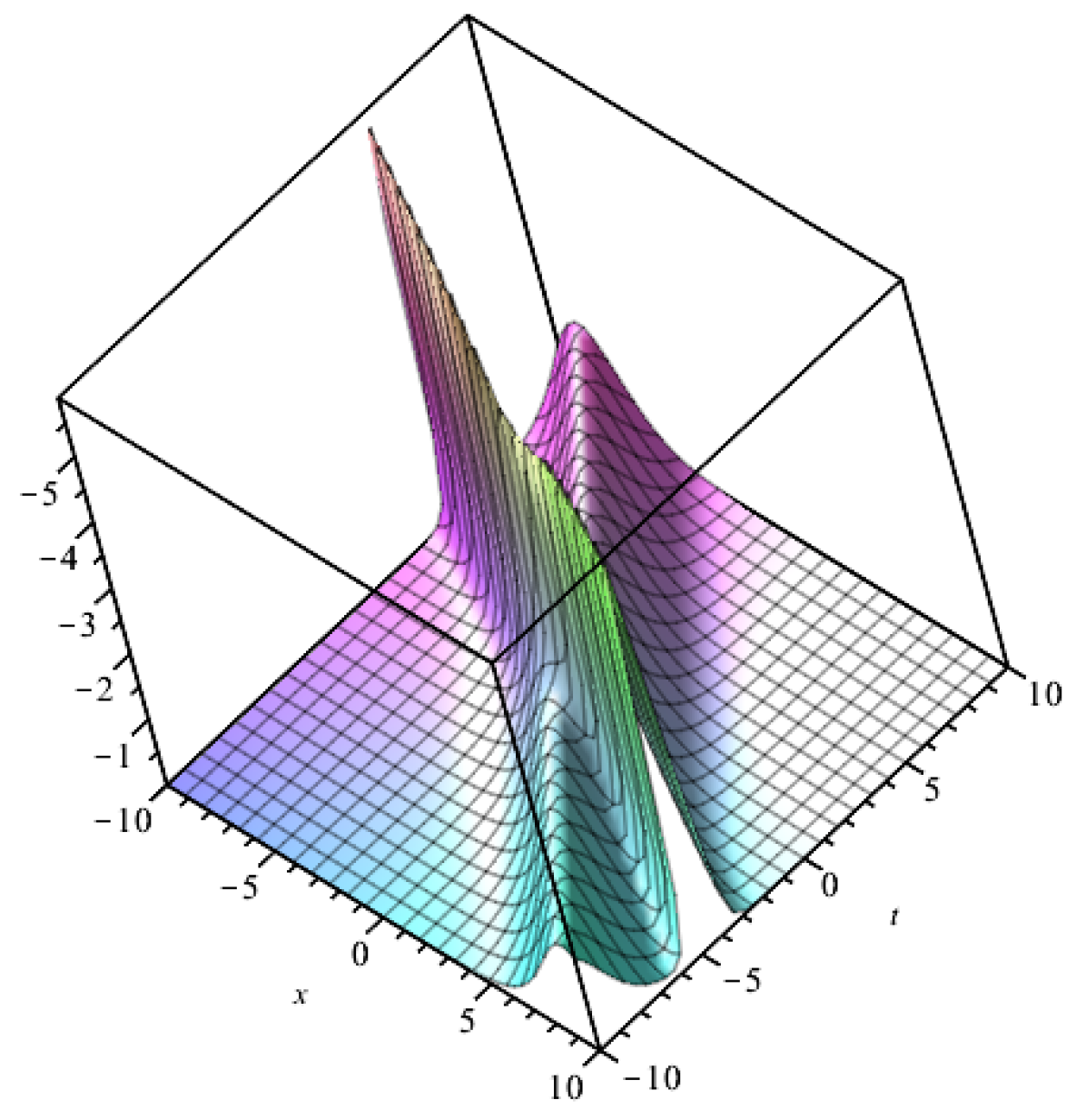
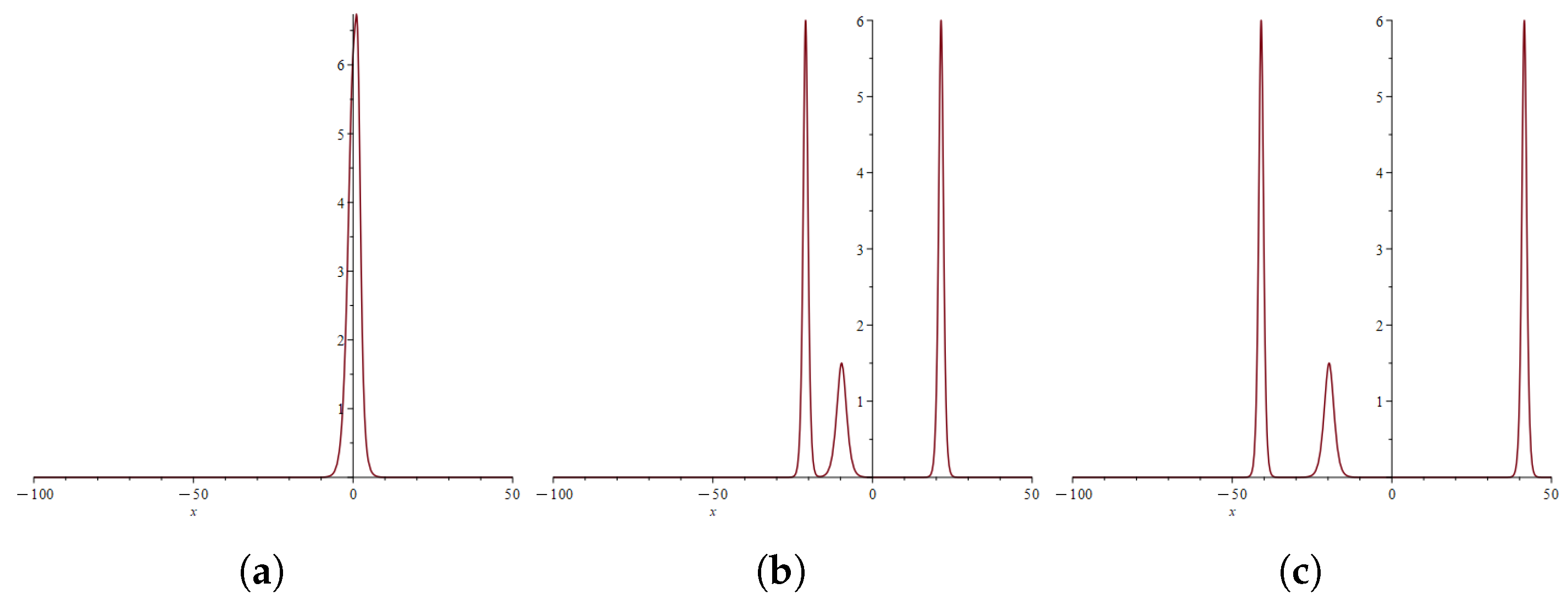
3.3. Verification of the Soliton Solution of the System

The Hirota bilinear method is now utilized to find the soliton solution to the (1 + 1)-dimensional Boussinesq equation. The Hirota bilinear form can be expressed as:

$$(D_t^2-D_x^4)f·f=2(f{f}_{xx}-f_x^2-f{f}_{xxxx}+4f_{xxx}{f}_x-3f_{xx}^2)=0.$$

(27)

Now do a perturbative expansion of f, we assume that:

$$f=1+\epsilon f_1+{\epsilon }^2{f}_2+{\epsilon }^3{f}_3+\cdots .$$

(28)

Bringing this into bilinear form and collecting the coefficients of each power of $\epsilon$ yields:

$$\begin{array}{cc}& {\epsilon }^0:(D_t^2-D_x^4)(1·1)=0,\hfill \\ & {\epsilon }^1:(D_t^2-D_x^4)(1·f_1+f_1·1)=0,\hfill \\ & {\epsilon }^2:(D_t^2-D_x^4)(1·f_2+f_2·1)=-(D_t^2-D_x^4)(f_1·f_1),\hfill \\ & {\epsilon }^3:(D_t^2-D_x^4)(1·f_3+f_3·1)=-(D_t^2-D_x^4)(f_1·f_2+f_2·f_1).\hfill \\ & \cdots \hfill \end{array}$$

(29)

The above system of partial differential equations is solved below. Since $(D_t^2-D_x^4)(1·f_1+f_1·1)=2f_{1xx}-2f_{1xxxx}=0$ is a linear partial differential equation with respect to $f_1$ which satisfies the superposition formula, it is assumed that:

$$f_1=\sum _{i=1}^N{e}^{{\xi }_i},{\xi }_i={\mu }_{i}x+{\omega }_{i}t+{\sigma }_i,i=1,2\dots ,N,$$

(30)

where ${\mu }_i,{\omega }_i,{\sigma }_i$ are parameters to be determined.

To obtain a one-soliton solution to the equation, taking $f_1=e^{{\xi }_1},{\xi }_1={\mu }_{1}x+{\omega }_{1}t+{\sigma }_1,$ and bringing it into the second equation yields:

$${\omega }_1={\mu }_1^2,$$

(31)

From this, we can conclude that $f_1=e^{{\mu }_{1}x+{\mu }_1^{2}t+{\sigma }_1}$, and bringing this into the coefficients of ${\epsilon }^2$ gives:

$$2f_{2xx}-2f_{2xxxx}=0,$$

(32)

and the equation has a zero solution $f_2=0$.

Similarly, taking $f_2$ and $f_3$ into the coefficients of ${\epsilon }^3$ yields $f_3=0$. By analogy, we obtain $f_n=0,n\ge 2$. Taking $\epsilon =1$ yields:

$$F_1=f=1+e^{{\xi }_1}=1+e^{{\mu }_{1}x+{\mu }_1^{2}t+{\sigma }_1}.$$

(33)

Bringing the above equation into the transformation $u=-6{(ln{F}_1)}_{xx}$, the one-soliton solution to the (1 + 1)-dimensional Boussinesq equation is obtained as:

$$u=-6{\displaystyle \frac{{\mu }_1^2{e}^{{\mu }_{1}x+{\mu }_1^{2}t+{\sigma }_1}}{{\left(1+e^{{\mu }_{1}x+{\mu }_1^{2}t+{\sigma }_1}\right)}^2}}.$$

(34)

The evolution of the one-soliton solution is further plotted (Figure 2) by selecting appropriate parameter values ${\mu }_1=1.5,{\sigma }_1=0.5$.

In order to investigate whether the waveform and amplitude of the one-soliton solution change with time, take the time t = 0, 10, 50 and obtain the two-dimensional plot as follows Figure 3:

It is not difficult to observe that the one-soliton solution of the (1 + 1)-dimensional Boussinesq equation possesses excellent properties: as time evolves, both its waveform and amplitude remain constant, with only a change in phase.

Next, the two-soliton solution to the equation is computed. When $N=2$, we take $f_1=e^{{\xi }_1}+e^{{\xi }_2},{\xi }_i={\mu }_{i}x+{\omega }_{i}t+{\sigma }_i,i=1,2,$ and taking it into the third equation yields:

$$f_{2tt}-f_{2xxxx}=[-{({\omega }_1-{\omega }_2)}^2+{({\mu }_1-{\mu }_2)}^4]e^{{\xi }_1+{\xi }_2}.$$

(35)

Then, we assume that $f_2=a_{12}{e}^{{\xi }_1+{\xi }_2}$, where $a_{12}$ is the coefficient to be determined. Substituting it into the Equation (35), we obtain:

$$a_{12}={\displaystyle \frac{-{({\omega }_1-{\omega }_2)}^2+{({\mu }_1-{\mu }_2)}^4}{{({\omega }_1+{\omega }_2)}^2-{({\mu }_1+{\mu }_2)}^4}}.$$

(36)

Similarly, we have ${\omega }_1={\mu }_1^2,{\omega }_2={\mu }_2^2$. Bringing the $f_1$ and $f_2$ obtained above into the coefficients of ${\epsilon }^3$ gives $f_3=0$ and similarly gives $f_n=0,n\ge 3$. Taking $\epsilon =1$ yields:

$$F_2=f=1+f_1+f_2=1+e^{{\xi }_1}+e^{{\xi }_2}+{\displaystyle \frac{-{({\omega }_1-{\omega }_2)}^2+{({\mu }_1-{\mu }_2)}^4}{{({\omega }_1+{\omega }_2)}^2-{({\mu }_1+{\mu }_2)}^4}}{e}^{{\xi }_1+{\xi }_2}.$$

(37)

Bringing the above equation into the transformation $u=-6{(ln{F}_1)}_{xx}$, the two-soliton solution to the (1 + 1)-dimensional Boussinesq equation can be obtained.

The evolution of the two-soliton solution is further plotted by selecting appropriate parameter values. By choosing ${\mu }_1=2,{\mu }_2=1,{\sigma }_1={\sigma }_2=0.5$, the results are obtained as follows (Figure 4).

In order to investigate whether the waveform and amplitude of the two-soliton solution change with time, take the time $t=0,10,50$ and obtain the two-dimensional plots as follows Figure 5:

From the above figures, it can be observed that at $t=0$, a one-soliton state is presented, followed by a collision between two soliton waves. This collision is manifested as two one-soliton solutions with different amplitudes and waveforms, moving towards the same direction at different speeds. Unlike the one-soliton solution, the case of the two-soliton solution is less stable.

Similarly, the three-soliton solutions of the equation can be found. When $N=3$, the three-soliton solution is $u=-6{(ln{F}_3)}_{xx}$, where

$$\begin{array}{cc}\hfill & F_3=f=1+f_1+f_2+f_3=1+e^{{\xi }_1}+e^{{\xi }_2}+e^{{\xi }_2}+a_{12}{e}^{{\xi }_1+{\xi }_2}+a_{13}{e}^{{\xi }_1+{\xi }_3}+a_{23}{e}^{{\xi }_2+{\xi }_3}+a_{123}{e}^{{\xi }_1+{\xi }_2+{\xi }_3},\hfill \\ \hfill & {\xi }_i={\mu }_{i}x+{\omega }_{i}t+{\sigma }_i,{\omega }_i={\mu }_i^2,i=1,2,3,a_{ij}={\displaystyle \frac{-{\left({\omega }_i-{\omega }_j\right)}^2+{\left({\mu }_i-{\mu }_j\right)}^4}{{\left({\omega }_i+{\omega }_j\right)}^2-{\left({\mu }_i+{\mu }_j\right)}^4}},a_{123}=a_{12}{a}_{13}{a}_{23}.\hfill \end{array}$$

(38)

Bringing the above equation into the transformation $u=-6{(ln{F}_1)}_{xx}$, the three-soliton solution to the (1 + 1)-dimensional Boussinesq equation can be obtained. The evolution of the three-soliton solution is plotted by further choosing appropriate parameter values (Figure 6).

In order to investigate whether the waveform and amplitude of the two-soliton solution change with time, take the time $t=0,10,20$ and obtain the two-dimensional plots as follows Figure 7:

From the above figures, it can be observed that at $t=0$, a one-soliton state is presented, followed by a collision between three soliton waves. This collision is manifested as two one-soliton solutions with the same amplitudes and waveforms and one one-soliton solution with a smaller amplitude, all moving towards the same direction at different speeds. Similar to the case of the two-soliton solution, the three-soliton solution is also less stable.

Similarly, we can derive the N-soliton solution of the (1 + 1)-dimensional Boussinesq equation as:

$$u=2[ln(\sum _{\eta =0,1}exp(\sum _{i=1}^n{\eta }_i{\xi }_i+\sum _{1\le i\le j}^n{\eta }_i{\eta }_j{a}_{ij})){]}_{xx},$$

(39)

where ${\sum }_{\eta =0,1}$ is all possible combinations of ${\eta }_i=0,1(i=1,2\cdots N)$ and ${\xi }_i={\mu }_{i}x+{\omega }_{i}t+{\sigma }_i$, and we obtain

$$a_{ij}={\displaystyle \frac{-{\left({\omega }_i-{\omega }_j\right)}^2+{\left({\mu }_i-{\mu }_j\right)}^4}{{\left({\omega }_i+{\omega }_j\right)}^2-{\left({\mu }_i+{\mu }_j\right)}^4}}.$$

(40)

When delving into the nonlinear dynamical characteristics of the (1 + 1)-dimensional Boussinesq equation, it is noteworthy for its unique mathematical structure in describing solitary wave phenomena. To verify the applicability of the model, this paper utilizes volatility data from Data1 (${\sigma }_{EGARCH}$) to estimate the parameter ${\mu }_i$ in the Boussinesq equation. Through least squares optimization, a value of ${\mu }_1=1.5$ is obtained (see Figure 2), which aligns with the observed price fluctuations in the empirical data. Furthermore, the solution to Equation (34) successfully reproduces the mean reversion phenomenon of carbon prices around their equilibrium value, thereby affirming the potential explanatory power of soliton theory within the carbon market. Specifically, the one-soliton solution of this equation exhibits high stability and conservation, manifesting as the physical parameters of the soliton, such as waveform, amplitude, and velocity, remaining constant during propagation. This property is referred to as “shape preservation” or “conservative evolution” in physics. Such dynamic consistency provides an ideal model framework for analyzing persistent wave patterns in complex systems.

Mapping this phenomenon to the financial sector, particularly in the study of carbon price fluctuations in the carbon trading market, reveals a profound analogy. Similar to how the one-soliton of the (1 + 1)-dimensional Boussinesq equation maintains its characteristic shape unchanged, the carbon price, after undergoing a period of changes, may exhibit a stable trend towards an equilibrium price. Even when subjected to short-term disturbances, it can recover to a certain determined price trajectory, reflecting a strong inherent self-regulating capability.

However, in scenarios involving the interaction of multiple solitons, the Boussinesq equation reveals a more complex dynamical behavior: collisions between solitons often result in their initial waveforms not being completely restored. This symbolizes the nonlinear responses and long-term effects that may arise from the intertwining influences of various factors in the carbon market, such as policy changes and shifts in supply/demand relationships. It indicates that the evolution path of carbon prices is not a simple superposition process but rather exhibits rich nonlinear dynamical characteristics.

4. Conclusions

Through the organic integration of empirical analysis and nonlinear system theory, this study provides an in-depth examination of the internal mechanisms driving fluctuations in carbon market prices. Utilizing data from the EU carbon quota (EUA) options market, we first apply the EGARCH model to demonstrate that the yield series of carbon futures exhibits a significant non-normal distribution (K-S test statistic $D=0.121,p<0.001$). This empirical finding serves as a crucial data foundation for subsequent development of nonlinear dynamic models.

In terms of theoretical modeling, we have innovatively incorporated the (1 + 1)-dimensional Boussinesq equation into our investigation of carbon price dynamics. Notably, it is essential to emphasize that the calibration process for model parameters is entirely grounded in the empirical analysis results presented earlier: volatility parameters estimated via the EGARCH model are directly mapped onto the coefficients of nonlinear terms within the Boussinesq equation, while characteristics such as thick tails in the yield series dictate the strength of dispersion terms within this framework. This data-driven modeling approach ensures a robust correlation between theoretical constructs and empirical findings.

The results indicate that nonlinear evolution equation theory effectively captures complex dynamics within carbon markets. Specifically, stability observed in soliton solutions aligns closely with mean reversion behaviors exhibited by carbon prices; additionally, amplitude conservation reflects underlying equilibrium mechanisms present within these markets. Furthermore, multi-soliton interactions accurately simulate nonlinear responses to price fluctuations triggered by policy shocks. These findings not only affirm the applicability of nonlinear system theory within financial environmental science but also offer a novel theoretical perspective on understanding operational patterns inherent to carbon markets.

Future research directions include further refining the data calibration methods for model parameters while considering the influence of additional market microstructure factors; exploring the potential applications of other types of nonlinear evolution equations in carbon market modeling; and developing a more accurate price prediction model based on this theoretical framework. These studies will enhance our understanding of carbon market operations and provide more robust scientific support for relevant policy-making.

References

1. Zhang, L.; Bai, E. The Regime Complexes for Global Climate Governance. Sustainability 2023, 15, 9077. [Google Scholar] [CrossRef]
2. Wang, A.L. Regulating domestic carbon outsourcing: The case of China and climate change. UCLA L. Rev. 2013, 61, 2018. [Google Scholar]
3. Fokas, A.S. Integrable nonlinear evolution equations in three spatial dimensions. Proc. R. Soc. A 2022, 478, 20220074. [Google Scholar] [CrossRef] [PubMed]
4. Liu, M.M.; Yu, J.P.; Ma, W.X.; Khalique, C.M.; Sun, Y.L. Dynamic analysis of lump solutions based on the dimensionally reduced generalized Hirota bilinear KP-Boussinesq equation. Mod. Phys. Lett. B 2023, 37, 2250203. [Google Scholar] [CrossRef]
5. Zhang, J.; Zhu, M.; Liu, S.; Li, C.; Wang, X. Bäcklund transformation, Lax pair, infinite conservation laws and exact solutions to a generalized (2+1)-dimensional equation. Int. J. Mod. Phys. B 2022, 36, 2250146. [Google Scholar] [CrossRef]
6. Yasmin, H.; Alshehry, A.S.; Ganie, A.H.; Mahnashi, A.M.; Shah, R. Perturbed Gerdjikov–Ivanov equation: Soliton solutions via Backlund transformation. Optik 2024, 298, 171576. [Google Scholar] [CrossRef]
7. Liu, Z.; Madhavan, V.; Tegmark, M. Machine learning conservation laws from differential equations. Phys. Rev. E 2022, 106, 045307. [Google Scholar] [CrossRef] [PubMed]
8. Chai, X.; Xu, L.; Sun, Y.; Liang, Z.; Lu, E.; Li, Y. Development of a cleaning fan for a rice combine harvester using computational fluid dynamics and response surface methodology to optimise outlet airflow distribution. Biosyst. Eng. 2020, 192, 232–244. [Google Scholar] [CrossRef]
9. Tang, P.; Li, H.; Issaka, Z.; Chen, C. Impact forces on the drive spoon of a large cannon irrigation sprinkler: Simple theory, cfd numerical simulation and validation. Biosyst. Eng. 2017, 159, 1–9. [Google Scholar] [CrossRef]
10. Jiang, Y.; Li, H.; Chen, C.; Xiang, Q. Calculation and verification of formula for the range of sprinklers based on jet breakup length. Int. J. Agric. Biol. Eng. 2018, 11, 49–57. [Google Scholar] [CrossRef]
11. Lu, E.; Ma, Z.; Li, Y.; Xu, L.; Tang, Z. Adaptive backstepping control of tracked robot running trajectory based on real-time slip parameter estimation. Int. J. Agric. Biol. Eng. 2020, 13, 178–187. [Google Scholar] [CrossRef]
12. Kang, W.; Lin, H.; Adade, S.; Wang, Z.; Ouyang, Q.; Chen, Q. Advanced sensing of volatile organic compounds in the fermentation of kombucha tea extract enabled by nano-colorimetric sensor array based on density functional theory. Food Chem. 2023, 405, 134193. [Google Scholar] [CrossRef]
13. Wang, J.; Chen, Q.; Belwal, T.; Lin, X.; Luo, Z. Insights into chemometric algorithms for quality attributes and hazards detection in foodstuffs using raman/surface enhanced raman spectroscopy. Compr. Rev. Food Sci. Food Saf. 2021, 20, 2476–2507. [Google Scholar] [CrossRef] [PubMed]
14. Yang, X.; Mi, J.; Zeng, Y.; Wei, W. Bilinear Integrable soliton solutions and carbon emission rights pricing. Int. J. Low-Carbon Technol. 2023, 18, 131–143. [Google Scholar] [CrossRef]
15. Dash, R.; Dash, P.K. An evolutionary hybrid Fuzzy Computationally Efficient EGARCH model for volatility prediction. Appl. Soft Comput. 2016, 45, 40–60. [Google Scholar] [CrossRef]
16. Liu, Z.; Huang, S. Research on pricing of carbon options based on GARCH and BS model. J. Appl. Sci. Eng. Innov. 2019, 6, 109–116. [Google Scholar]
17. Stoev, S.; Taqqu, M.S.; Park, C.; Marron, J.S. On the wavelet spectrum diagnostic for Hurst parameter estimation in the analysis of Internet traffic. Comput. Netw. 2005, 48, 423–445. [Google Scholar] [CrossRef]
18. Massey, F.J., Jr. The Kolmogorov-Smirnov test for goodness of fit. J. Am. Stat. Assoc. 1951, 46, 68–78. [Google Scholar] [CrossRef]
19. Jaiswal, S.; Jaiswal, T. Review on machine learning techniques for stock-market forecasting. Artif. Intell. Evol. 2020, 1, 34–47. [Google Scholar] [CrossRef]
20. Tapkın, S.; Çevik, A.; Uşar, Ü. Accumulated strain prediction of polypropylene modified marshall specimens in repeated creep test using artificial neural networks. Expert Syst. Appl. 2009, 36, 11186–11197. [Google Scholar] [CrossRef]
21. Dong, H.; Zhao, K.; Yang, H.; Li, Y. Generalised (2+1)-dimensional super MKdV hierarchy for integrable systems in soliton theory. East Asian J. Appl. Math. 2015, 5, 256–272. [Google Scholar] [CrossRef]
22. Jiang, J.; Li, W.; Cai, X.; Wang, Q. Empirical study of recent Chinese stock market. Phys. Stat. Mech. Its Appl. 2009, 388, 1893–1907. [Google Scholar] [CrossRef]
23. Lou, S.Y.; Jia, M. From one to infinity: Symmetries of integrable systems. J. High Energy Phys. 2024, 2024, 1–10. [Google Scholar] [CrossRef]
24. Xu, G.; Li, Z. Symbolic computation of the Painlevé test for nonlinear partial differential equations using Maple. Comput. Phys. Commun. 2004, 161, 65–75. [Google Scholar] [CrossRef]
25. Wang, C. Lump solution and integrability for the associated Hirota bilinear equation. Nonlinear Dyn. 2017, 87, 2635–2642. [Google Scholar] [CrossRef]
26. Yan, S.; Li, C. Explicit solutions from Darboux transformation for the two-component nonlocal Hirota and Maxwell-Bloch system. Int. J. Geom. Methods Mod. Phys. 2023, 20, 2350062. [Google Scholar] [CrossRef]
27. Gaillard, P. Degenerate Riemann theta functions, Fredholm and wronskian representations of the solutions to the KdV equation and the degenerate rational case. J. Geom. Phys. 2021, 161, 104059. [Google Scholar] [CrossRef]
28. Dong, P.; Ma, Z.Y.; Fei, J.X.; Cao, W. The shifted parity and delayed time-reversal symmetry-breaking solutions for the (1 + 1)-dimensional Alice-Bob Boussinesq equation. Front. Phys. 2023, 11, 1137999. [Google Scholar] [CrossRef]
29. Ma, W.X.; Zhang, Y.; Tang, Y.; Tu, J. Hirota bilinear equations with linear subspaces of solutions. Appl. Math. Comput. 2012, 218, 7174–7183. [Google Scholar] [CrossRef]
30. Léger, F.; Li, W. Hopf-Cole transformation via generalized Schrödinger bridge problem. J. Differ. Equ. 2021, 274, 788–827. [Google Scholar] [CrossRef]
31. Nolte, B.; SchäFer, I.; Ehrlich, J.; Ochmann, M.; Marburg, R.B.A.S. Numerical methods for wave scattering phenomena by means of different boundary integral formulations. J. Comput. Acoust. 2007, 15, 495–529. [Google Scholar] [CrossRef]
Figure 1. Descriptive statistical analysis of yield.
Mathematics 13 01304 g001
Figure 2. Three-dimensional plot of the one-soliton solution.
Mathematics 13 01304 g002
Figure 3. Two-dimensional plot of one-soliton solution.
Mathematics 13 01304 g003
Figure 4. Three-dimensional plot of two-soliton solution.
Mathematics 13 01304 g004
Figure 5. Two-dimensional plots of two-soliton solution when: (a) t = 0, (b) t = 10, (c) t = 50.
Mathematics 13 01304 g005
Figure 6. Three-dimensional plot of the three-soliton solution.
Mathematics 13 01304 g006
Figure 7. Two-dimensional plots of three-soliton solution when: (a) t = 0, (b) t = 10, (c) t = 20.
Mathematics 13 01304 g007