1. Introduction
Longitudinal data are characterized by repeated and correlated measurements across multiple covariates. Such data are ubiquitous in disciplines such as biomedical research, econometrics, and social sciences [
1]. In [
2], the authors highlighted prominent applications in these domains and discussed specialized statistical methodologies for analyzing longitudinal data. Conventional approaches are designed primarily for independent observations, and often fail to account for the intrinsic dependencies in longitudinal settings, resulting in biased parameter estimates and compromised inferential validity. Thus, advancing robust techniques that explicitly model the correlation structures of longitudinal data remains a critical methodological priority.
The generalized estimating equation (GEE) method [
3] represents a cornerstone approach for longitudinal data analysis, offering consistent estimation through the incorporation of a working correlation structure. While this framework provides robustness against misspecification of the within-cluster correlation matrix, its validity critically depends on the mechanism used for missing data. Specifically, the GEE estimator may exhibit substantial bias when observations are missing not at random or missing at random, rather than missing completely at random. This limitation underscores the necessity of developing more sophisticated methodologies capable of addressing non-random missingness in longitudinal studies. In longitudinal data analysis, informative cluster size (ICS) occurs when the conditional expectation of the response variable depends on the cluster size [
4], a phenomenon also termed nonignorable cluster size. This issue arises frequently in applied settings. For example, the number of patient follow-up visits in clinical studies may correlate with disease severity. Formally, we can let
X denote the covariates,
Y represent the response variable (e.g., disease status), and
M indicate the cluster size (e.g., number of visits). The ICS condition be formulated as
, which implies that standard analyses ignoring
M may yield biased inferences. Similarly, observation frequency at sampling sites in ecological studies may depend on environmental factors. Another example arises in toxicology experiments where pregnant dams are randomly exposed to toxicants. Sensitive dams may produce litters with a higher rate of birth defects and experience more fetal resorptions, resulting in smaller litter sizes.
To address these challenges, Ref. [
4] proposed the within-cluster resampling (WCR) method for marginal analysis of longitudinal data. This approach involves randomly selecting a single observation per cluster (with replacement) and applying standard inference techniques for independent data. The WCR method offers two key advantages over conventional GEE method. First, it is robust against correlation misspecification. By analyzing resampled independent observations, WCR inherently accommodates within-cluster correlations, thereby avoiding biases arising from misspecified working correlation structures. In contrast, the GEE method can produce unreliable estimates when the assumed correlation matrix is incorrect [
5] or when the true dependence structure is complex or unknown. Second, WCR maintains validity in the presence of nonignorable cluster size. Unlike GEE, which implicitly weights observations by cluster size, WCR eliminates this weighting scheme by treating each cluster equally through resampling. This property ensures consistent estimation even when cluster sizes are informative about the response variable, as WCR’s resampling mechanism inherently adjusts for ICS. Thus, WCR provides a principled framework for valid inference in settings where traditional GEE may fail due to either correlation misspecification or nonignorable cluster sizes.
Recent methodological developments have significantly advanced the analysis of high-dimensional longitudinal data, particularly in addressing the dual challenges of variable selection and parameter estimation. In [
6], the authors introduced a Bayesian information criterion (BIC)-based selection approach using quadratic inference functions, while Ref. [
7] developed corresponding asymptotic theory for binary outcomes when the number of predictors grows with cluster size. Building on this foundation, Ref. [
8] proposed penalized generalized estimating equations (PGEE) with the smoothly clipped absolute deviation (SCAD) penalty [
9], enabling simultaneous variable selection and estimation under specified moment conditions and working correlation structures. Parallel innovations include [
10]’s quadratic decorrelated inference function for high-dimensional inference and [
11]’s one-step debiased estimator via projected estimating equations, which facilitates hypothesis testing for linear combinations of high-dimensional coefficients. These contributions collectively provide a robust statistical framework for analyzing complex longitudinal data, helping to bridge critical gaps between theoretical development and practical application.
However, these GEE-based approaches critically depend on accurate estimation of within-cluster correlations, rendering them vulnerable to performance inconsistencies when informative cluster size (ICS) is present. To address this limitation, researchers have developed estimation techniques within the WCR framework. For instance, Ref. [
12] introduced a modified WCR approach aimed at improving estimation efficiency, though requiring clusters of size greater than one and imposing further constraints on the correlation structure. Additionally, Ref. [
13] developed a resampling-based cluster information criterion for finite-dimensional semiparametric marginal mean regression. A naive yet essential strategy is to generate the final estimation by averaging a substantial quantity of resampled estimators. Specifically, when
R resamplings are conducted, the WCR estimator is calculated as
, where
is obtained from the
rth resampled data set for
. Nevertheless, this averaging strategy presents significant theoretical limitations in high-dimensional settings. On one hand, the method provides no formal guarantees for consistent model selection in high-dimensional regression problems; On the other, the unregularized averaging process may retain noise variables, potentially leading to model overfitting [
14].
In this study, we introduce a novel model selection procedure tailored for high-dimensional longitudinal data in the presence of ICS. The dimension of covariates, denoted as
, is permitted to grow exponentially with the number of clusters
n. Leveraging the stability that the WCR framework provides in finite-dimensional settings under ICS, we aim to extend its applicability to scenarios where the number of covariates surpasses the total number of clusters while ensuring both model selection and estimation consistency. Our proposed penalized likelihood via WCR approach (abbreviated as
) combines penalized likelihood with WCR through three key steps. For resampling, following [
4], we draw one observation per cluster (with replacement), creating
n independent samples. For regularized estimation, we perform simultaneous variable selection and parameter estimation for each of
R resamples via penalized likelihood maximization, utilizing the resulting
n independent observations of resampling data sets. Finally, for stable aggregation, we prevent overfitting from naive averaging by applying component-wise penalized mean regression across the
R estimates, producing a sparse final model. This integrated framework maintains WCR’s robustness to ICS while addressing high-dimensional challenges through proper regularization.
Our approach offers three distinct improvements over existing longitudinal data approaches. (i) Correlation-robust inference: naturally handles intracluster dependence without explicit correlation modeling while avoiding estimation bias from misspecified correlation structures, This is especially crucial in higher dimensions. (ii) ICS-robust estimation: Our method maintains robustness even when dependencies exist between the response variables and cluster sizes, effectively addressing the challenges associated with ICS. (iii) Stable sparse recovery: By incorporating penalized mean regression during aggregation, ensures sparse solutions and significantly reduces overfitting risk versus naive averaging These advantages collectively enhance the reliability and applicability of the proposed method in complex longitudinal data analyses.
The rest of this paper is structured as follows.
Section 2 presents the model framework, examines the limitations of GEE estimation, and details our methodology. Theoretical guarantees of the proposed estimator under mild regularity conditions are established in
Section 3. Comprehensive simulation results appear in
Section 4, followed by an application to yeast cell-cycle gene expression data in
Section 5. We conclude with discussion of broader implications in
Section 6, while technical proofs are collected in the
Appendix A.
Below, we introduce the notation commonly used throughout this paper. For any constant a, its integer part is denoted by . For any vector and , we define , , , , and . For any subset of the row index set of , denotes the cardinality of and represents the subvector of corresponding to the indices in , with the indicator function denoted by . Let be an matrix and let be its inverse. For subsets , denotes the submatrix of formed by column indices in and represents the submatrix with rows and columns indexed by and , respectively. The maximum and minimum eigenvalues of a matrix are denoted by and , respectively, while the spectral norm is provided by .
3. Theoretical Properties
In this section, we establish the consistency of model selection and parameter estimation.
For convenience, we first introduce some notation. Let be the index set corresponding to the nonzero components in . We define , , and . We denote and . Let and .
The following regularity conditions are required for establishing asymptotic results.
- (A1)
Let for . Assume that is increasing and concave in and that it has a continuous derivative with . In addition, is independent of ; for simplicity, we write it as .
- (A2)
(i) for some positive constants and .
(ii) for any , where .
- (A3)
Assume that for any there exist some positive constants and such that and holds with probability going to one.
- (A4)
Assume that , and .
- (A5)
Define the supremum of the local concavity of
as
and suppose that
.
Condition (A1) is satisfied by commonly used folded concave penalty functions such as LASSO [
15], SCAD [
9], and MCP [
16] (with
). In [
9], the authors state that an ideal estimator should be equipped with three desirable properties: unbiasedness, sparsity, and continuity. However, the LASSO penalty fails to reach an unbiased estimator, the
penalty with
does not produce a sparse solution, and the
penalty with
does not satisfy the continuous condition. In our study, SCAD penalty is chosen to conduct variable selection. Its derivative is defined as
for some
and
. This penalty satisfies both Condition (A1) and the three desirable properties within the penalized likelihood framework.
Condition (A2) restricts the moment of errors and the sub-Gaussian distribution of the predictors to satisfy this condition, which is commonly used for high-dimensional penalized regression [
17,
18,
19]. Condition (A2)(i) holds for the exponential generalized linear model family (1).
In Condition (A3), the singular value constraint
and
is the same as
and
in [
17], which has been proven for the family of exponential generalized linear models in [
18] when the covariate vector follows from a sub-Gaussian distribution. Furthermore,
is the unrepresentable condition [
20], which is commonly assumed for penalized regression.
Condition (A4) restricts the strength of signals, number of nonzero covariates, dimension of the feature space, and tuning parameter, which is commonly used in [
17,
18]. From Condition (A4), we allow
,
, which is a common condition for ultra-high-dimensional feature spaces in the literature. Finally, Condition (A5) is assumed by [
17] in order to ensure the second-order condition.
The following theorem establishes the oracle property of the penalized likelihood estimator via WCR.
Theorem 1. Assume that Conditions (A1)–(A5) hold. Then, we have and as , where .
Theorem 1 establishes model selection sparsity and the estimation consistency of . It also holds for the ultra-high-dimensional feature space regardless of whether or not the cluster size is informative.
In the following, we establish the oracle property of the penalized likelihood estimator via WCR.
Theorem 2. Assume that the conditions in Theorem 1 all hold. If satisfies and , then we have and as , where .
Compared to the penalized GEE method proposed by [
8], our
method demonstrates several significant advantages in handling high-dimensional longitudinal data with informative cluster sizes.
First,
substantially improves model selection accuracy, particularly in the presence of ICS. By adopting the WCR framework described in [
4], our method assigns equal weights to observations from clusters of varying sizes, thereby ensuring robustness when the cluster sizes are related to outcomes. Repeated marginal analyses conducted on resampled datasets allow us to fully utilize sample information while maintaining consistent screening results. The subsequent aggregation of
R candidate models through component-wise penalized least squares further enhances the reliability of our approach. Importantly, this aggregation process ensures that occasional omissions of important covariates in individual analyses do not substantially affect the final estimates, while repeated misidentification of noise variables is effectively suppressed. As a result,
achieves a higher true positive rate while simultaneously reducing false positives. This represents a distinct advantage over the PGEE method, which relies on a single model fitting that provides each variable with only one selection opportunity, and is consequently more vulnerable to selection errors.
Second, offers superior handling of within-cluster correlations without requiring explicit specification of the correlation structure. Though computationally intensive, the WCR approach effectively circumvents the need to estimate potentially complex intracluster correlation structures. This represents a significant improvement over the PGEE method, where accurate estimation critically depends on within-cluster correlations. This requirement often proves problematic, particularly in nonlinear cases where correlation estimates may be invalid. The implicit treatment of correlation in not only simplifies implementation but also enhances the method’s robustness across diverse data scenarios. These combined advantages position as a more reliable and versatile tool for high-dimensional longitudinal data analysis compared to existing penalized GEE approaches.
4. Simulation Studies
In this section, we describe a series of numerical experiments evaluating the performance of the proposed
method in model selection for longitudinal data. The tuning parameter within the penalized likelihood is selected by minimizing the extended Bayesian information criterion (BIC) [
21], ensuring an optimal balance between model complexity and goodness of fit. In the aggregation step, we investigate several different choices of resampling time (
), providing sensitivity analyses to demonstrate the robustness and tradeoffs between computational efficiency and stability, on the basis of which we choose
times resampling for the most robust and reliable results. Furthermore, with the exception of LASSO, we explore the SCAD penalty as an alternative sparse penalty function in order to elucidate potential improvements or limitations. We use five-fold cross-validation to select
in (
8) for each
. In addition, we compare the aggregation performance of the simple averaging method. Specifically, we take the average of the resulting
R estimated values for each covariate component. These experiments aimed to validate the effectiveness and stability of our
approach in handling high-dimensional longitudinal data with informative cluster sizes.
In this study, we compare our proposed method with two competing approaches. The first is the penalized GEE (PGEE) method introduced by [
8], which is implemented using the R package
PGEE. Three commonly used working correlation structures are considered: independence, exchangeable (equally correlated), and autoregressive of order 1 (AR-1). To facilitate a clear comparison of these methods under different correlation scenarios, we append the suffixes “.indep”, “.exch”, and “.ar1” to denote the independence, exchangeable, and AR-1 correlation structures, respectively. As recommended by [
8], the PGEE method is executed over 30 iterations and a fourfold cross-validation procedure is employed to select the tuning parameter in the SCAD penalty function. Additionally, following [
8], a coefficient is identified as zero if its estimated magnitude falls below the threshold value of
. This comparative framework ensures a rigorous evaluation of the proposed method’s performance relative to established approaches. Additionally, we consider a simplified approach that neglects within-cluster correlation and applies a penalized maximum likelihood with the
-penalty, referred to as naive LASSO. This method serves as a baseline for comparison, particularly in scenarios where intracluster dependencies are ignored. Our investigations encompass both correlated continuous and binary response variables.
Notably, the penalized generalized estimating equations (PGEE) method requires approximately 4 h to fit a single generated dataset, even when the covariate dimension is as low as 50. In contrast, our proposed method completes the same task in just 5 min, demonstrating significantly improved computational efficiency. Due to the substantial time demands of PGEE, we exclude its performance evaluation for datasets with . This omission highlights the practical advantages of our approach in high-dimensional settings where computational efficiency is critical.
We generate 100 longitudinal datasets for each setup. To evaluate the screening performance, we calculate the following criteria: (1) true positive (TP), the average number of true variables that are correctly identified; (2) false positive (FP), the average number of unimportant variables that are selected by mistake; (3) coverage rate (CR), the probability that the selected model covers the true model; and (4) mean square error (MSE), calculated as , where is the estimate obtained on the rth generated dataset. All algorithms were run on a computer with an Intel(R) Xeon(R) Gold 6142 CPU and 256 GB RAM.
Example 1. In this example, we consider the underlying model asfor correlated normal responses with ICS, where and . The random cluster size takes a value in the set , with the probability distribution as , , and . Here, we define . The -dimensional vector of covariates are independently generated from a multivariate normal distribution, which has mean 0 and an autoregressive covariance matrix with marginal variance 1 and autocorrelation . The coefficient vector presents a homogeneous effect. The random errors obey a multivariate normal distribution with marginal mean 0, marginal variance 1, and an exchangeable correlation matrix with parameter . In Example 1, we control the ICS severity by introducing a univariable
, leading to
which is not equal to
Since the distribution of
depends on the cluster size
, the marginal expectation of the responses is also influenced by
. By adjusting the distributions of
and
, the severity of informative cluster size (ICS) can be modified.
Table 1 presents a comparative summary of model selection performance and estimation accuracy for the three competing methods in Example 1. While all methods successfully identify the TPs, only our
method consistently selects a model that closely approximates the true sparse structure. For
, the PGEE method incorporates a small number of redundant variables under the three commonly used working correlation structures. Similarly, the naive LASSO approach selects a moderately sized model, particularly when the within-cluster correlation increases to
. Notably,
method achieves the smallest mean squared error (MSE) while demonstrating robustness against increases in both model dimension and intracluster correlation. In contrast, PGEE exhibits significant inconsistency in the presence of ICS, with estimation errors nearly doubling as the within-cluster correlation intensifies. Furthermore, naive LASSO produces biased estimates and displays sensitivity to the dimension of the covariates, resulting in a substantially larger MSE. These findings underscore the superior performance of our
method in high-dimensional longitudinal data analysis under ICS.
Table 2 provides model selection and parameter estimation results at
and
for Example 1 with varying resampling times, two alternative aggregation penalties, and the simple averaging method. For linear regression, LASSO exhibits decreasing FPs and relatively robust MSE with increased resampling times. SCAD retains zero FPs and equally efficient estimates to LASSO. When compared with conventional
regularization, the SCAD penalty possesses a superior sparsity-inducing property. However, simple averaging aggregation yields non-sparse models. With increasing sampling frequency, a growing number of redundant variables with weak signals are identified.
Example 2. In this example, we consider correlated binary responses with marginal mean satisfyingwhere and . To account for ICS, we let the random cluster size follow the probability distribution as , , and . The components of the covariates vector are jointly normal distributed with mean 0 and an autoregressive covariance matrix. The covariance matrix has marginal variance 1 and autocorrelation 0.4. We set . The correlated binary responses were generated using the R package
SimCorMultRes
using an exchangeable within-cluster correlation parameter . Correlated binary outcomes inherently contain less information than continuous data, posing greater challenges when seeking to accurately identify significant variables and obtain precise estimates. The model selection and estimation results for Example 2 are summarized in
Table 3. Notably, the proposed
method consistently identifies all relevant features while maintaining model sparsity across all scenarios. In contrast, the PGEE method struggles to identify the true model under an independent correlation structure, with the CR rate dropping below 60%. Although PGEE achieves asymptotic consistency under the other two intracluster correlation structures, this comes at the expense of higher FPs compared to our method. Furthermore, naive LASSO exhibits some deficiencies in identifying TPs when the covariates are autoregressively correlated with a coefficient of
. In the presence of ICS, the MSE of our
method experiences minor adverse effects but remains the lowest among the three competing methods. For
, PGEE produces severely biased estimates when the observations are assumed to be independent. Even when the working correlation structure is correctly specified, the MSE of PGEE is approximately three times higher than that of
. Meanwhile, naive LASSO demonstrates significant bias and yields the largest MSE, highlighting its limitations in handling correlated binary outcomes under ICS. These results underscore the robustness and precision of our
method in high-dimensional longitudinal data analysis with binary responses.
Sensitivity analyses of Example 2 at
and
are presented in
Table 4. Obviously, LASSO shows slight FPs in contrast to SCAD’s constant zero FPs. For binary outcomes, the SCAD penalty demonstrates negligible estimation deviations compared with LASSO at
. The estimation errors plateau as
R increases, indicating that the aggregation effect becomes independent of the penalty function when the resampling times reach 500. This demonstrates that our proposed
method exhibits asymptotic robustness with respect to the number of resamplings. Unlike binary models, simple averaging aggregation generates a substantial number of redundant variables, which severely compromises estimation efficiency and doubles the MSE of the estimates.
The performance of the penalized GEE approach varies under different working correlation structures (independence, exchangeable, and autoregressive), particularly in the presence of informative cluster size (ICS). Even when the working correlation structure is correctly specified, the resulting estimates can still show substantial bias, as illustrated in
Table 1 and
Table 3. The naive LASSO method is also affected by both intracluster correlations and ICS. In practice, the true within-cluster correlation structure is often complex and challenging to identify. To address these issues, our proposed
method leverages within-cluster resampling to simultaneously account for intricate correlation patterns and ICS, leading to more robust model selection and parameter estimation. Moreover, the proposed
method maintains its robustness across different levels of dimensionality from
to 500 thanks to the stabilizing effect of aggregation. In contrast, the penalized GEE fails to produce a sparse model, while naive LASSO suffers from considerable estimation bias even at moderate dimensionality
.
In Examples 3 and 4, we intentionally exclude ICS in order to evaluate the robustness of the proposed method under scenarios where ICS is not a factor. This design allows us to isolate and examine the method’s performance in handling high-dimensional longitudinal data without the confounding influence of ICS, providing a clearer assessment of its general applicability and stability. By focusing on these examples, we aim to demonstrate that our method remains effective even in the absence of ICS, thereby further validating its utility across diverse longitudinal data settings.
Example 3. We consider the linear modelfor correlated normal responses, where , . The values of are generated following the same procedure as in Example 1. The coefficient vector is specified as , representing a homogeneous effect. The covariates are generated according to the method described in Example 1. The random errors follow a multivariate normal distribution with marginal mean 0, marginal variance 1, and exchangeable correlation matrix characterized by a parameter . Table 5 summarizes the model selection and estimation results for continuous correlated responses in Example 3. Overall, the proposed
method successfully identifies all relevant covariates while achieving the most parsimonious model size among the competing methods. Under the data generation mechanism specified in Example 3, the PGEE method also provides a sparse selected model and optimal estimation, particularly when assuming a pairwise equal correlation structure. This is because the generalized estimating equations (GEE) approach provides consistent and efficient estimates of regression coefficients while accounting for within-cluster dependencies. GEE utilizes all available observations and adjusts for intracluster correlation. When the a priori specified working correlation structure approximates the true dependence, the GEE estimator achieves optimal efficiency, minimizing the asymptotic variance of parameter estimates. Our simulation results demonstrate that GEE maintains type I error control and statistical power. In comparison, the MSEs of the
method are comparable to those of PGEE, indicating that our method also enjoys robust performance regardless of ICS. In contrast, naive LASSO selects moderately sized models but produces biased estimates, with the bias becoming more pronounced at
.
When combined with the results from Example 1, it is apparent that the proposed method demonstrates robust model selection performance and accurate estimation regardless of whether ICS is ignorable. These findings highlight the versatility and reliability of our approach in handling high-dimensional longitudinal data across diverse scenarios.
In
Table 6, it can be seen that the results of the sensitivity analyses for Example 3 are similar to those in Example 1 at
and
. After eliminating the influence of ICS, all three aggregation methods exhibit significant improvements in estimation efficiency. Although simple averaging substantially reduces the FPs in the absence of nonignorable cluster sizes, the selected model remained non-sparse. The model selection performance of the linear models exhibits little sensitivity to variations in the sampling frequency.
Example 4. In this example, we model the correlated binary responses with the marginal mean defined aswhere and . The random cluster sizes and covariates are generated following the procedure described in Example 2. The coefficient vector is set as . The observations within each cluster exhibit an exchangeable correlation structure with parameter . Table 7 provides a summary of the model selection results and estimation accuracy for the competing methods in Example 4. When the correlated binary responses are independent of the cluster size, our proposed
method consistently outperforms alternative approaches in both signal identification and parameter estimation. While the PGEE method exhibits instability in terms of TPs and FPs across different working correlation matrices, it demonstrates improvement in identifying significant features compared to its performance in Example 2. Although the naive LASSO method is able to achieve model sparsity, its performance is inferior to the proposed approach due to its biased parameter estimation. As the number of covariates increases to
, our
method continues to excel, selecting an oracle model with the smallest MSE. These results underscore the robustness and precision of our
method in handling high-dimensional longitudinal data with binary responses even in the absence of ICS.
Table 8 summarizes the results of the sensitivity analyses for Example 4 at
and
. While increasing
R reduces parameter estimation errors, this improvement comes at the cost of elevated computational demands. Notably, our experiments demonstrate nearly equivalent performance between
and
, suggesting diminishing returns beyond
. When combined, the results from
Table 2,
Table 3,
Table 4,
Table 5,
Table 6,
Table 7 and
Table 8 show that 500 times resampling for our
method achieves good robustness and tradeoffs between computational efficiency and stability.
5. Yeast Cell-Cycle Gene Expression Data Analysis
In this section, we assess the performance of our proposed
method using a subset of the yeast cell-cycle gene expression dataset compiled by [
22]. This dataset comprises 292 cell-cycle-regulated genes with expression levels monitored across two complete cell-cycle periods. Repeated measurements were collected for these 292 genes at intervals of 7 min over a span of 119 min, yielding a total of 18 time points. This dataset provides a valuable opportunity to evaluate the efficacy of our method in analyzing high-dimensional longitudinal data with inherent temporal dependencies.
The cell-cycle process is typically divided into a number of distinct stages: M/G1, G1, S, G2, and M. The M (mitosis) stage involves nuclear events such as chromosome separation as well as cytoplasmic events such as cytokinesis and cell division. The G1 (GAP 1) stage precedes DNA synthesis, while the S (synthesis) stage is characterized by DNA replication. The G2 (GAP 2) stage follows synthesis, and prepares the cell for mitosis. Transcription factors (TFs) play a crucial role in regulating the transcription of a subset of yeast cell-cycle-regulated genes. In [
23], the authors utilized ChIP data from [
24] to estimate the binding probabilities for these 292 genes, covering a total of 96 TFs.
To identify the TFs that are potentially involved in the yeast cell-cycle, we consider the following model:
where
represents the log-transformed gene expression level of gene
i measured at time point
j for
and
. The variable
denotes the matching score of the binding probability of the
dth TF for gene
i at time point
j. Previous studies have highlighted the importance of interaction effects among certain TFs, such as HIR1:HIR2 [
25], SWI4:SWI6 [
26], FKH2:NDD1 [
27], SWI5:SMP1 [
28], MCM1:FKH2 [
29], MBP1:SWI6 [
26], and FKH1:FKH2 [
29,
30]. Given this evidence, the model in (
9) is well justified, resulting in a total of 4656 covariates for analysis.
As discussed in
Section 4, we compare the variable selection performance of the proposed
method with that of the PGEE and naive LASSO methods.
Table 9 summarizes the identification results for 21 transcription factors (TFs) that have been experimentally verified and are known to be associated with the yeast cell cycle (referred to as “true” TFs) [
23]. This comparison highlights the ability of each method to accurately identify biologically relevant TFs, providing insights into their respective strengths and limitations in the context of high-dimensional longitudinal data analysis. The proposed
method demonstrates superior performance in identifying true TFs while maintaining model sparsity, further validating its utility in biological applications. Overall, the proposed
method selects the smallest number of TFs while identifying 17 “true” TFs, which is the highest count among all competing methods. In contrast, PGEE exhibits variable performance depending on the assumed within-cluster correlation structures. When observations are modeled as independent or equally correlated, PGEE identifies 11 “true” TFs out of 60 and 61 selected TFs, respectively. Under an autoregressive correlation structure, PGEE improves slightly, identifying 15 “true” TFs among 60 selected TFs. These results underscore the strong dependence of PGEE’s performance on the choice of working correlation structure. Meanwhile, the naive LASSO method identifies 12 “true” TFs from a comparable total number of selected TFs. These findings highlight the robustness and precision of our
method in accurately identifying biologically relevant TFs while maintaining model sparsity, even in the presence of complex correlation structures.
Next, we examine the identification of specific ”true” TFs in more detail. All of the competing methods successfully select ACE2, CBF1, FKH1, MBP1, NDD1, REB1, STB1, SWI4, and SWI5.
- •
BAS1: BAS1 is known to regulate the synthesis of histidine, purines, and pyrimidines [
31], and also plays a role in preparing yeast cells for division. However, the penalized GEE method fails to identify it as important.
- •
MCM1: This TF primarily exerts its regulatory effects during the M/G1, S, and early G2 stages, indicating its critical role in the yeast cell cycle. Although it is identified as one of the three major TF types by [
22], MCM1’s vital impact is overlooked by the penalized GEE method.
- •
MET31: MET31 is required for interactions with the activator MET4 to bind DNA. It regulates sulfur metabolism [
32], a process linked to the initiation of cell division [
33]. Notably, only our
method identifies the importance of MET31.
Despite achieving sparsity, the naive LASSO method fails to select several significant TFs with substantial biological roles:
- •
FKH2, which plays a dominant role in regulating genes associated with nuclear migration and spindle formation [
34].
- •
SWI6, which coordinates gene expression at the G1-S boundary of the yeast cell cycle, as noted by [
35].
These results highlight the superior performance of the proposed
method in reliably identifying critical TFs associated with the yeast cell cycle. However, a few TFs were not successfully detected by
.
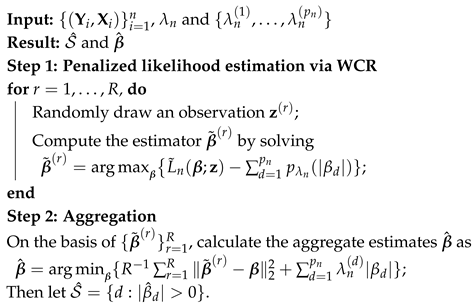
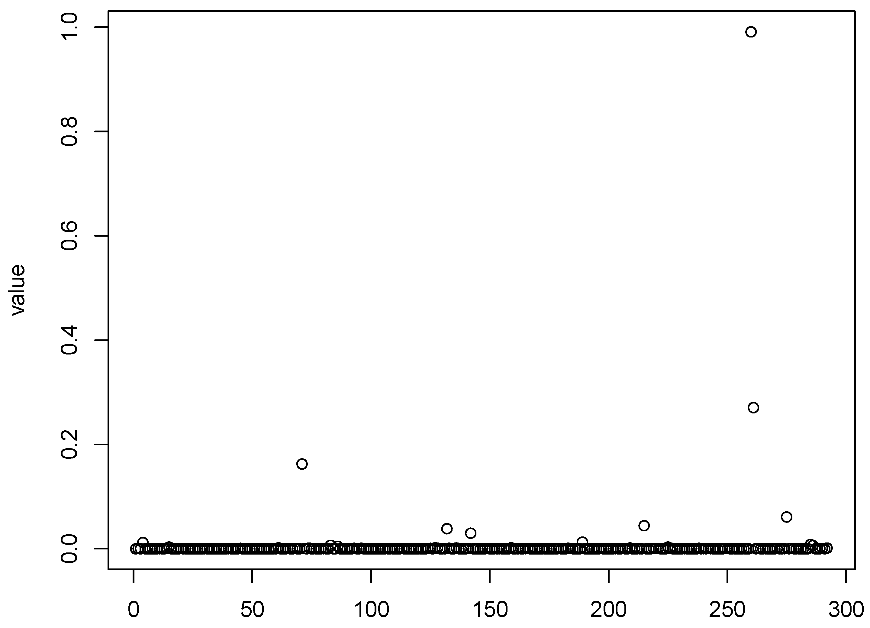
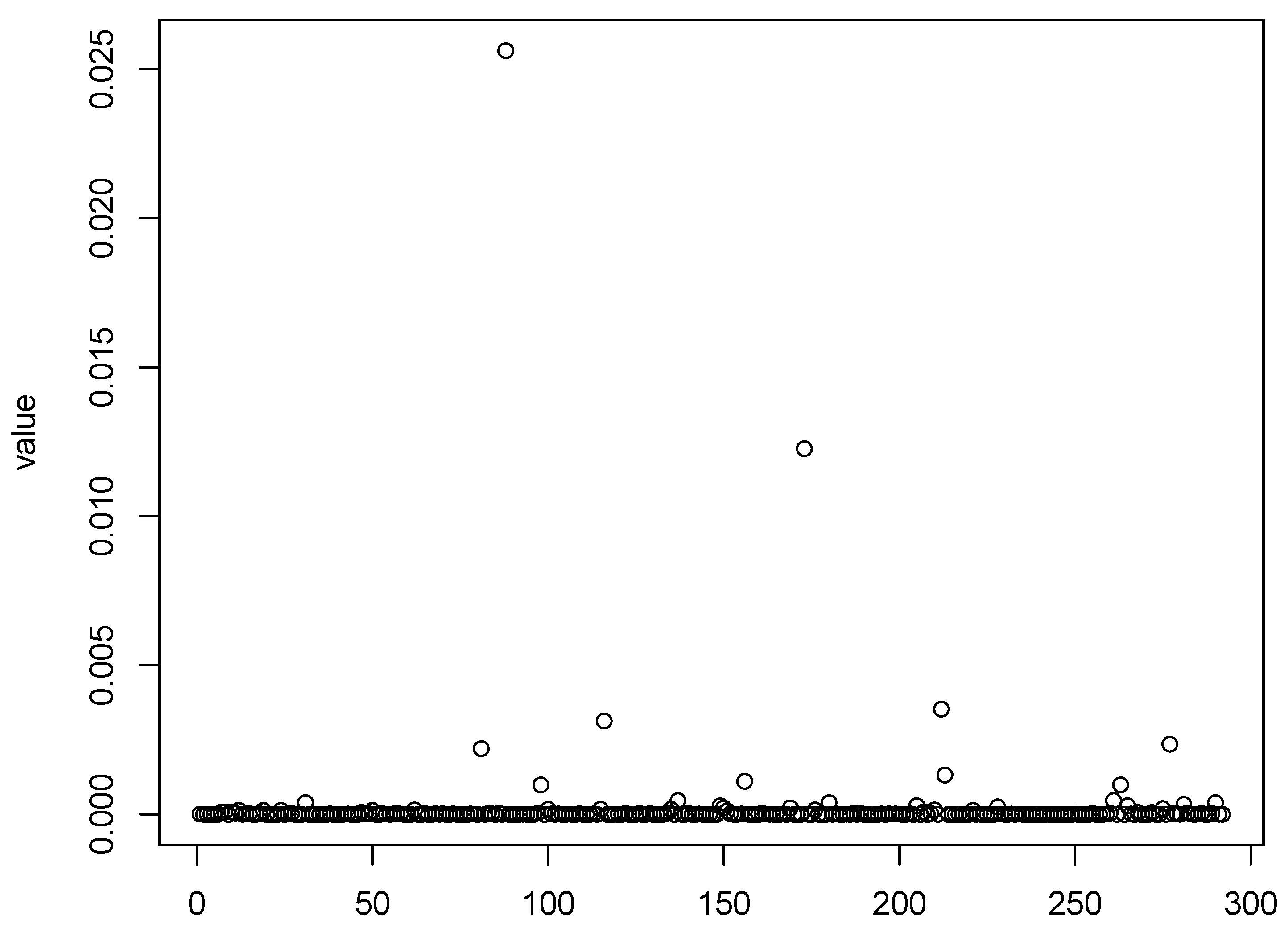
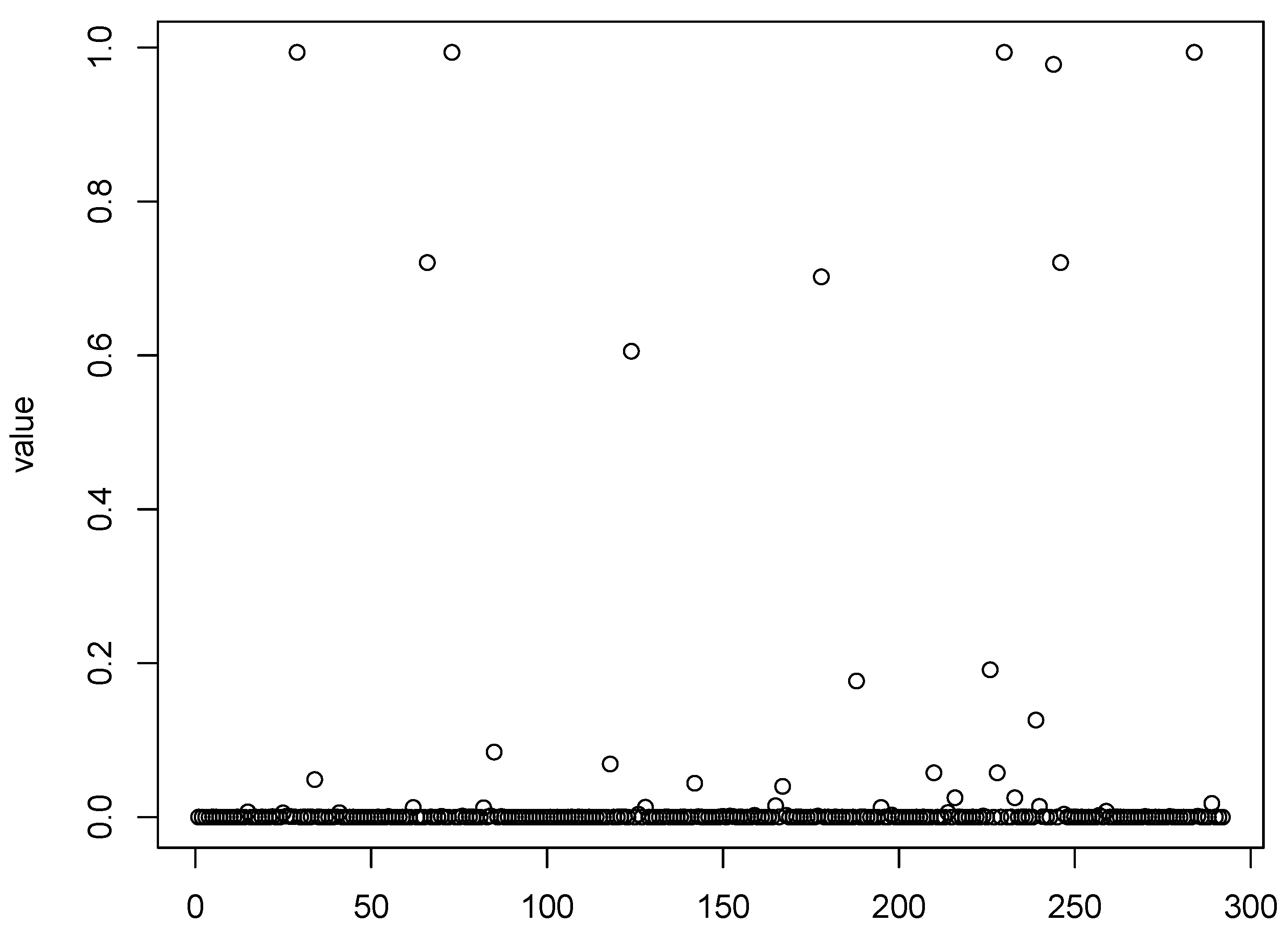
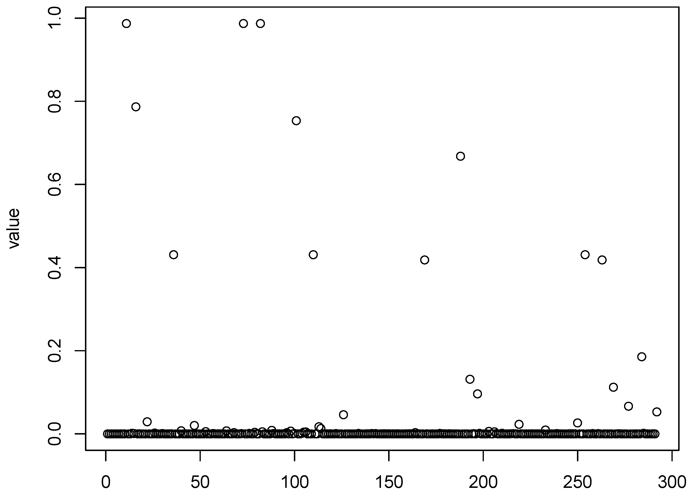
Figure 1,
Figure 2,
Figure 3 and
Figure 4 show scatter plots of the matching score of the binding probability of four missing “true” TFs: GCN4, GCR1, SKN7, and STE12, respectively. A common characteristic can be observed among these TFs in that the majority of observations are clustered near zero, with only a limited number of outliers exhibiting deviations. This phenomenon results in our resampling-based penalized estimation approach misclassifying these TFs as invariant constants rather than as variables, causing their exclusion from the identified set. In particular, GCR1 displayed an exceptionally low variance (on the order of
), effectively approximating a constant zero expression level.
Notably, GCN4 was not identified as significant by any of the considered methods. The naive LASSO method was the only approach to select GCR1, while SKN7 and STE12 were recognized as cell cycle regulators exclusively by the PGEE method. To better understand these discrepancies, we turn to relevant biological research for plausible explanations. First, GCN4, which was not detected by any method, may play a regulatory role under specific conditions or stress responses that are not fully captured in the current dataset. Similarly, GCR1 was identified only by naive LASSO, and might exhibit weak or context-dependent regulatory effects that are more challenging to detect using methods that account for within-cluster correlations. The identification of SKN7 and STE12 by PGEE but not by could be attributed to the sensitivity of PGEE to specific correlation structures, which may align more closely with the regulatory patterns of these TFs.
Relevant biological research can offer plausible explanations that may aid in better understanding these discrepancies. First, the heterogeneous regulatory effects of TFs during the yeast cell cycle likely contribute to these observations. Different TFs exhibit varying levels of regulatory involvement at distinct stages of the cycle. Furthermore, certain TFs regulate the cell cycle in a periodic manner, with their effects confined to specific intervals. Because our
method samples observations at arbitrary time points, it tends to prioritize TFs with consistent regulatory effects across the two observed periods. For example, STE12 is known to regulate the cyclic expression of certain genes specifically during the early G1 phase, as documented by [
36]. This phase represents a relatively narrow time window, resulting in a low sampling probability and an estimated coefficient close to zero. However, if observations were specifically sampled during the G1 phase, STE12 could be successfully identified. This highlights the importance of considering temporal dynamics and stage-specific regulatory mechanisms when analyzing cell-cycle-related gene expression data.
Additionally, the complex interactions between transcription factors (TFs) may influence the identification results. For instance, SKN7 exhibits several genetic interactions with MBP1 during the G1-S transition, including mutual inhibition [
37]. Despite this interaction, our
method identified MBP1 as significant, potentially overshadowing SKN7. This suggests that the regulatory influence of MBP1 as captured by the model may dominate or mask the effects of SKN7 due to their antagonistic relationship. Such intricate interaction between TFs underscores the challenges in disentangling their individual contributions and highlights the need for more sophisticated modeling approaches.
In addition to the 21 experimentally verified TFs, our
method also identified additional regulatory TFs with biological evidence supporting their roles in the yeast cell cycle. For example, HIR1 is known to be involved in the cell cycle-dependent repression of histone gene transcription [
38]. Similarly, [
39] demonstrated that PHD1 contributes to centriole duplication and centrosome maturation, playing a critical role in regulating cell cycle progression. These findings not only validate the accuracy of our
method in identifying biologically relevant TFs but also highlight its potential to uncover additional regulatory factors that may have been overlooked by other approaches. This underscores our proposed method’s utility in advancing the understanding of complex biological processes such as cell cycle regulation.


