Event-Based Quantized Dissipative Filtering for Nonlinear Networked Systems

Abstract

This article investigates the event-based dissipative filtering problem for nonlinear networked systems with dynamic quantization. The nonlinear plant is represented using a discrete-time Takagi–Sugeno (T–S) fuzzy model. The main idea of this article is that a novel dynamic event-triggered mechanism as well as a dynamic quantization strategy combined with a general online adjustment rule are introduced to comprehensively decrease the amount of data involved in network communication and realize the rational utilization of limited communication resources. This article aims to design an event-based quantized filter such that the asymptotic stability and the specified dissipative filtering performance of the filtering error system can be ensured. The design conditions for the desired filter are provided in the form of linear matrix inequalities. Lastly, the effectiveness of the proposed filter design method is demonstrated through the simulation results of a practical example.

1. Introduction

Over the last fifteen years, research on networked systems has garnered attention from numerous scholars. Compared to traditional control systems, networked systems offer advantages such as lower cost, easier maintenance, and convenient scalability. Networked systems have been widely used in the fields of unmanned driving, aerospace, robotics, and so on [1]. In the real world, the bandwidth of communication networks is limited, and excessive redundant data transmission can lead to significant wastage of communication resources. Therefore, reducing the network communication burden without compromising system performance is a key problem to be addressed by scholars and engineers. After continuous research, the event-triggered strategy and quantization scheme have emerged as two of the most effective approaches to addressing the limited bandwidth of communication networks. Moreover, many noteworthy results on networked systems featuring the event-triggered strategy or quantization scheme have been published. The design issues associated with networked systems based on the event-triggered strategy have been studied by many scholars and a number of valuable papers have been published, such as [2,3,4,5]. According to the quantization scheme, the design issues for networked systems have been studied by researchers in [6,7,8].

On the other hand, in industrial production, the vast majority of systems are nonlinear. Compared to linear systems, nonlinear systems exhibit higher complexity, require more intricate stability analysis, and imply more challenging control design [9,10]. Therefore, many scholars have studied nonlinear systems. Among them, as an effective method for addressing the design problems of nonlinear systems, the Takagi–Sugeno (T–S) fuzzy model strategy has become a research focus in the field of control [11,12,13,14]. Consequently, many articles addressing design problems of nonlinear systems based on the T–S fuzzy model strategy have been published. For example, fuzzy controller design issues have been discussed for nonlinear networked systems based on the event-triggered strategy in [15,16] and according to the quantization scheme in [17,18,19,20,21]; issues pertaining to control in nonlinear networked systems based on the event-triggered strategy and the quantization scheme have been studied in [22,23,24].

In addition to the aforementioned issues, the study of filtering is both theoretically and practically important in the control area [25,26]. As a result, many interesting results have been published over the past two decades. For linear networked systems, the authors in [27] studied the quantized filtering issue, the authors in [28,29] discussed the event-triggered filtering issue, and the authors in [30,31] addressed the issue of event-triggered filtering with quantization. Similarly, the filtering issue for T–S fuzzy systems has also received significant attention from researchers, and many valuable research results have been published (see, e.g., [32,33] and references therein). For nonlinear networked systems, the quantized fuzzy filtering issue was addressed in [34,35,36,37,38] and the issue of event-triggered fuzzy filtering was discussed in [39,40]. However, as two of the most significant methods for utilizing limited communication resources reasonably and effectively, the event-triggered strategy and the quantization scheme were not considered in the above results simultaneously. However, the event-triggered strategy and the quantization scheme were employed to deal with the fuzzy filtering issue for nonlinear networked systems in [41,42,43,44]. It is worth noting that the event-triggered strategy or the quantization scheme used in [41,42,43,44] cannot be adjusted dynamically. By introducing the threshold function and the online adjustment rule, the event-triggered strategy and quantization strategy can be improved, thereby enabling efficient utilization of limited communication resources. As a result, it is important to investigate the fuzzy filtering issue for nonlinear networked systems based on the dynamic event-triggered strategy and dynamic quantization scheme, which motivates our study.

In contrast with the published research results, this article contributes the following:

(1) In this article, the dissipative filtering problem is studied for nonlinear networked systems based on a dynamic event-triggered strategy and dynamic quantization scheme.

(2) A modified dynamic event-triggered strategy and a dynamic quantization scheme combined with an improved adjusting scheme are employed to reduce the communication burden.

The remainder of this article is composed of the following sections. The main content of Section 2 focuses on the problem formulation. Section 3 presents the design results. Simulation examples are presented in Section 4 of this article. In Section 5 of the article, the entire article is summarized.

2. Problem Formulation

A block diagram of the nonlinear networked systems considered in this article is given in Figure 1. Subsequently, the considered dissipative filtering problem is formulated in detail.

2.1. Nonlinear Plant

The discrete-time T–S fuzzy model will be utilized to model the nonlinear plant studied in this article and the j-th rule is presented as follows.

Plant Rule j: If $m_1\left(k\right)$ is $N_{1j}$ and $m_2\left(k\right)$ is $N_{2j}$ … and $m_{\partial \left(k\right)}$ is $N_{\partial j}$, then

$$\begin{array}{c}x(k+1)=A_{j}x\left(k\right)+B_{j}w\left(k\right)\hfill \\ y\left(k\right)=C_{j}x\left(k\right)+D_{j}w\left(k\right)\hfill \\ z\left(k\right)=E_{j}x\left(k\right)+F_{j}w\left(k\right)\hfill \end{array}$$

(1)

where $N_{pj}$ with $p=1,2,\dots ,\partial$ and $j=1,2,\dots ,i$ stand for the fuzzy sets, i is the number of fuzzy rules, and $m\left(k\right)=[m_1\left(k\right),m_2\left(k\right),\dots ,m_{\partial }\left(k\right)]$ is the premise variable. $x\left(k\right)\in {\mathfrak{R}}^{n_x}$ is the system state and $y\left(k\right)\in {\mathfrak{R}}^{n_y}$ is the measurement output. $w\left(k\right)\in {\mathfrak{R}}^{n_w}$ denotes the noise signal belonging to $l_2[0,\infty )$ and $z\left(k\right)\in {\mathfrak{R}}^{n_z}$ denotes the performance output. $A_j\in {\mathfrak{R}}^{n_x\times n_x}$, $B_j\in {\mathfrak{R}}^{n_x\times n_w}$, $C_j\in {\mathfrak{R}}^{n_y\times n_x}$, $D_j\in {\mathfrak{R}}^{n_y\times n_w}$, $E_j\in {\mathfrak{R}}^{n_z\times n_x}$, and $F_j\in {\mathfrak{R}}^{n_z\times n_w}$ represent system matrices.

Denote

$${\mu }_j\left(m\left(k\right)\right)={\displaystyle \prod _{p=1}^{\partial }}{N}_{pj}\left(m_p\left(k\right)\right),j=1,2,\dots ,i$$

(2)

where $N_{pj}\left(m_p\left(k\right)\right)$ represents the grade of membership of $m_p\left(k\right)$ in $N_{pj}$.

This assumes that

$${\mu }_j\left(m\left(k\right)\right)>0,{\displaystyle \sum _{j=1}^i}{\mu }_j\left(m\left(k\right)\right)>0,j=1,2,\dots ,i.$$

(3)

Let

$${\theta }_j\left(m\left(k\right)\right)={\displaystyle \frac{{\mu }_j\left(m\left(k\right)\right)}{{\sum }_{\nu =1}^i{\mu }_{\nu }\left(m\left(k\right)\right)}},j=1,2,\dots ,i.$$

(4)

Then

$${\theta }_j\left(m\left(k\right)\right)\ge 0,{\displaystyle \sum _{j=1}^i}{\theta }_j\left(m\left(k\right)\right)=1,j=1,2,\dots ,i.$$

(5)

Furthermore, the T–S fuzzy model in (1) can be further described as

$$\begin{array}{c}x(k+1)=A\left(\theta \right)x\left(k\right)+B\left(\theta \right)w\left(k\right)\hfill \\ y\left(k\right)=C\left(\theta \right)x\left(k\right)+D\left(\theta \right)w\left(k\right)\hfill \\ z\left(k\right)=E\left(\theta \right)x\left(k\right)+F\left(\theta \right)w\left(k\right)\hfill \end{array}$$

(6)

where

$$\begin{array}{c}A\left(\theta \right)={\displaystyle \sum _{j=1}^i}{\theta }_j\left(m\left(k\right)\right)A_j,B\left(\theta \right)={\displaystyle \sum _{j=1}^i}{\theta }_j\left(m\left(k\right)\right)B_j,\hfill \\ C\left(\theta \right)={\displaystyle \sum _{j=1}^i}{\theta }_j\left(m\left(k\right)\right)C_j,D\left(\theta \right)={\displaystyle \sum _{j=1}^i}{\theta }_j\left(m\left(k\right)\right)D_j,\hfill \\ E\left(\theta \right)={\displaystyle \sum _{j=1}^i}{\theta }_j\left(m\left(k\right)\right)E_j,F\left(\theta \right)={\displaystyle \sum _{j=1}^i}{\theta }_j\left(m\left(k\right)\right)F_j.\hfill \end{array}$$

2.2. Dynamic Event-Triggered Mechanism and Dynamic Quantizer

It can be observed from Figure 1 that both the event-triggered strategy and the dynamic quantizer will be employed to reduce the communication burden and realize the rational and efficient utilization of limited communication resources in this article.

According to the results developed in [3,4,44], a modified dynamic event-triggered strategy will be proposed, where the event-triggered condition is defined as follows:

$$\begin{array}{c}{\displaystyle \frac{1}{\omega }}\kappa \left(k\right)\le v^T\left(k\right){\varphi }_{1}v\left(k\right)-\lambda y^T\left(k_m\right){\varphi }_{2}y\left(k_m\right)\hfill \end{array}$$

(7)

where $0\le \lambda \le 1$ and $\omega >0$ are used to denote two predetermined parameters. $v\left(k\right)=y\left(k\right)-y\left(k_m\right)$ with $y\left(k_m\right)$ indicating the last transmitted measurement output. ${\varphi }_1>0$ and ${\varphi }_2>0$ represent two weighting matrices to be determined. In addition, $\kappa \left(k\right)$ is utilized to stand for the threshold function and the definition of $\kappa \left(k\right)$ is presented as

$$\begin{array}{c}\begin{array}{c}\kappa (k+1)=\varrho \kappa \left(k\right)-v^T\left(k\right){\varphi }_{1}v\left(k\right)+\lambda y^T\left(k_m\right){\varphi }_{2}y\left(k_m\right)\end{array}\hfill \end{array}$$

(8)

where $\kappa \left(0\right)={\kappa }_0$ denotes the initial condition of the threshold function and ${\kappa }_0\ge 0$. $0<\varrho <1$ stands for a predetermined parameter. Moreover, based on the results in [3,4], it can be obtained that $\kappa \left(k\right)\ge 0$ for all k as long as $\omega \varrho \ge 1$ is satisfied.

Remark 1. 

In contrast with the well-known static event-triggered strategy employed in [30,41,43]—i.e., a predefined event-triggered condition is utilized to determine whether the related data should be transmitted—the dynamic one proposed in this article is more general. The main reason for this is that the dynamic event-triggered strategy in this paper is able to adjust the event-triggered condition in (7) dynamically based on the threshold function in (8) with the parameters ω, λ, and ϱ to further reduce the communication burden. More specifically, it can be obtained from (7) and (8) that if the parameter λ increases and the parameters ω and ϱ decrease, fewer measurement outputs will satisfy the event-triggered condition in (7)—i.e., the communication burden will be reduced. Furthermore, it should be noted that the modified dynamic event-triggered strategy proposed in this article will reduce to the static one utilized in [41,43] by assuming $\omega \to \infty$ and ${\varphi }_1$ = ${\varphi }_2$; the dynamic event-triggered strategy employed in [44] can also be obtained from the one developed one herein by supposing ${\varphi }_1$ = ${\varphi }_2$.

The dynamic quantization scheme proposed in [8] will be adopted in this article, based on the results in [8]; a static quantizer will be defined that satisies the following two constraints:

$$\begin{array}{c}\left|g\right(\wp )-\wp |\le \Delta ,\mathrm{IF}|\wp |\le \mathcal{M}\hfill \end{array}$$

(9)

$$\begin{array}{c}\left|g\right(\wp )-\wp |>\Delta ,\mathrm{IF}|\wp |>\mathcal{M}\hfill \end{array}$$

(10)

where $\Delta >0$ indicates the quantization error bound of the quantizer and $\mathcal{M}>0$ indicates the quantization range of the quantizer. Then, the employed dynamic quantizer herein can be expressed as

$$\begin{array}{c}\tilde{y}\left(k\right)=\alpha g\left({\displaystyle \frac{y\left(k_m\right)}{\alpha }}\right)\hfill \end{array}$$

(11)

with $\alpha >0$ indicating the dynamic parameter.

Remark 2. 

As mentioned in [1,22,23], the main idea of the quantization scheme is to discretize the quantized signal in the sense of amplitude. In this way, only a small amount of data after discretization will be transmitted, which means that the communication burden will be partly reduced. In addition, it should be noted that the dynamic quantization scheme adopted in this article is more general than the static one employed in [27,30,36]. The main reason is that only a finite amount of quantization levels will be necessary to ensure the asymptotic stability of the filtering error system.

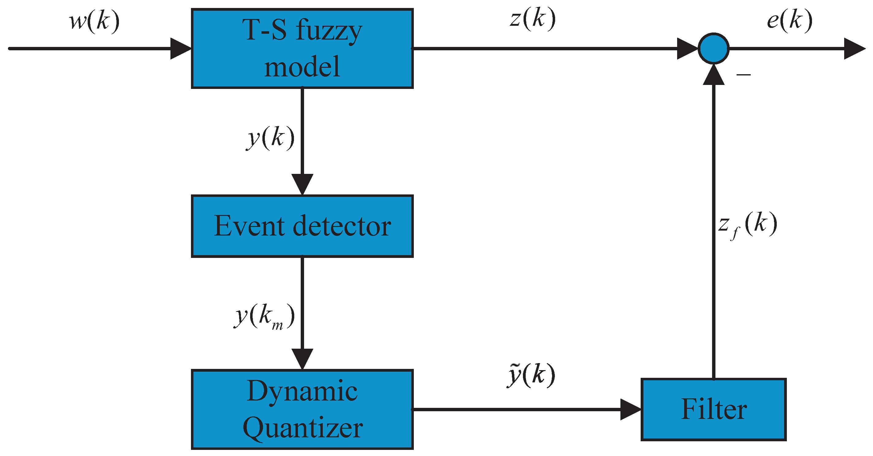
2.3. Filtering Error Systems

In order to realize the objective of estimating the system state, a filter will be constructed as follows:

$$\begin{array}{c}{x}_f(k+1)={\Psi }_A{x}_f\left(k\right)+{\Psi }_B\tilde{y}\left(k\right)\hfill \\ z_f\left(k\right)={\Psi }_E{x}_f\left(k\right)\hfill \end{array}$$

(12)

where $x_f\left(k\right)$ signifies the state of the filter and $z_f\left(k\right)$ indicates the output of the filter. ${\Psi }_A\in {\mathfrak{R}}^{n_x\times n_x}$, ${\Psi }_B\in {\mathfrak{R}}^{n_x\times n_y}$, and ${\Psi }_E\in {\mathfrak{R}}^{n_z\times n_x}$ are the parameters of the filter to be designed.

Remark 3. 

For the study of the control/filtering problem of fuzzy systems, the most effective approach is the parallel distributed compensation (PDC) scheme. As is well known, the precondition of the PDC scheme in [11,12,13] is that the membership functions are measurable. However, by considering the effects of the event-triggered mechanism and quantization, the PDC scheme is infeasible in this article. The main reason is that the membership functions will also be affected by the event-triggered mechanism and quantization before being transmitted to the filter. As a result, the membership functions in the filter and the plant will be different even though we assume that the membership functions are measurable. In summary, a quadratic filter is adopted herein rather than a fuzzy filter based on the PDC scheme.

Based on the equations in (6), (7), (11), and (12), the filtering error system can be obtained as follows:

$$\begin{array}{c}\psi (k+1)={\widehat{\mathbb{A}}}_{\chi }\psi \left(k\right)+{\widehat{\mathbb{B}}}_{\chi }w\left(k\right)+{\widehat{\mathbb{C}}}_{\chi }{\beta }_y\left(k\right)-{\widehat{\mathbb{C}}}_{\chi }v\left(k\right)\hfill \\ e\left(k\right)={\widehat{\mathbb{E}}}_{\chi }\psi \left(k\right)+{\widehat{\mathbb{F}}}_{\chi }w\left(k\right)\hfill \end{array}$$

(13)

where

$$\begin{array}{c}{\widehat{\mathbb{A}}}_{\chi }=\left[\begin{array}{cc}A\left(\theta \right)& 0\\ {\Psi }_{B}C\left(\theta \right)& {\Psi }_A\end{array}\right],{\widehat{\mathbb{B}}}_{\chi }=\left[\begin{array}{c}B\left(\theta \right)\\ {\Psi }_{B}D\left(\theta \right)\end{array}\right],\hfill \\ {\widehat{\mathbb{C}}}_{\chi }=\left[\begin{array}{c}0\\ {\Psi }_B\end{array}\right],{\widehat{\mathbb{E}}}_{\chi }=\left[\begin{array}{cc}E\left(\theta \right)& -{\Psi }_E\end{array}\right],\hfill \\ {\widehat{\mathbb{F}}}_{\chi }=F\left(\theta \right),{\beta }_y\left(k\right)=\alpha \left(g\left({\displaystyle \frac{y\left(k_m\right)}{\alpha }}\right)-{\displaystyle \frac{y\left(k_m\right)}{\alpha }}\right),\hfill \\ e\left(k\right)=z\left(k\right)-z_f\left(k\right),{\psi }^T\left(k\right)=\left[x^T\left(k\right)x_f^T\left(k\right)\right].\hfill \end{array}$$

Before proposing the dissipative filtering problem studied in this article, the following definition is given.

Definition 1 

([41]). Suppose that $L_1=L_1^T\in {\mathfrak{R}}^{n_e\times n_e}\le 0$, $L_2\in {\mathfrak{R}}^{n_e\times n_w}$, and $L_3=L_3^T\in {\mathfrak{R}}^{n_w\times n_w}$ are given matrices and $-L_1=L_{11}^T{L}_{11}$ with $L_{11}\in {\mathfrak{R}}^{n_e\times n_e}\ge 0$. Then, for $\varsigma \ge 0$ and the zero initial condition, the filtering error system in (13) is strict dissipativity with the dissipativity performance bound $\gamma >0$ as long as the inequality

$$\begin{array}{c}{\displaystyle \sum _{k=0}^{\varsigma }}\left(e^T\left(k\right)L_{1}e\left(k\right)+e^T\left(k\right)L_{2}w\left(k\right)+w^T\left(k\right)L_2^{T}e\left(k\right)\right.\hfill \\ \left.+w^T\left(k\right)(L_3-\gamma I)w\left(k\right)\right)\ge 0\hfill \end{array}$$

(14)

is satisfied.

Remark 4. 

It is worth noting that the definition for dissipative filtering performance in Definition 1 includes the following special cases.

(1) If $L_{11}=I$, $L_2=0$, and $L_3=({\gamma }^2+\gamma )I$, the definition for the $H_{\infty }$ filtering performance can be obtained from Definition 1.

(2) If $L_{11}=0$, $L_2=I$, and $L_3=2\gamma I$, the definition for the passive filtering performance can be obtained from Definition 1.

(3) If $L_{11}=\sqrt{b}I$, $L_2=(1-b)I$, and $L_3=(b({\gamma }^2-\gamma )+2\gamma )I$ with $0\le b\le 1$, the definition for the mixed passive/$H_{\infty }$ filtering performance can be derived from Definition 1.

In this article, the objective is to design the filter in (12) to guarantee the asymptotic stability as well as the dissipative filtering performance defined in Definition 1 of the filtering error system in (13).

3. Main Results

3.1. Filtering Performance Analysis

In this section, the analytic problem of the dissipative filtering performance for the filtering error system in (13) will be considered. Specifically, if the parameters of the filter in (12) are known, an analytic criterion of the dissipative filtering performance will be established in the following theorem characterized by two inequalities such that the asymptotic stability and the specified dissipative filtering performance of the filtering error system in (13) can be guaranteed.

Theorem 1. 

For given scalars $0<{\ell }_1\le {\ell }_2$ and $0<{𝚤}_1\le {𝚤}_2$, satisfying $1\le {𝚤}_1{\ell }_1$, $0\le \lambda \le 1$, $\omega >0$, $0<\varrho <1$, the quantization range $\mathcal{M}>0$, the quantization error bound $\Delta >0$, and matrices $L_1=L_1^T\le 0$, $L_2$, and $L_3=L_3^T$, if there exist scalars $\eta >1$, $\phi >0$, and ${\zeta }_1>0$ and matrices $P>0$, ${\varphi }_1>0$, and ${\varphi }_2>0$ that satisfy

$${\displaystyle \frac{{\ell }_1}{\mathcal{M}}}\le \phi \le {\displaystyle \frac{{\ell }_2}{\mathcal{M}}}$$

(15)

$$\left[\begin{array}{cccc}{\Phi }_{11}& \ast & \ast & \ast \\ {\Phi }_{21}& -P^{-1}& \ast & \ast \\ {\Phi }_{31}& 0& -I& \ast \\ {\Phi }_{41}& 0& 0& -{\zeta }_1^{-1}I\end{array}\right]<0$$

(16)

where

$$\begin{array}{c}{\Phi }_{11}=\left[\begin{array}{cccc}{\Gamma }_{11}& \ast & \ast & \ast \\ {\Gamma }_{12}& {\Gamma }_{22}& \ast & \ast \\ 0& 0& -{\zeta }_{1}I& \ast \\ -\lambda l{\varphi }_2\overline{C}& -\lambda l{\varphi }_2\overline{D}& 0& {\Gamma }_{44}\end{array}\right],\hfill \\ {\Phi }_{21}=\left[\begin{array}{cccc}{\widehat{\mathbb{A}}}_{\chi }& {\widehat{\mathbb{B}}}_{\chi }& {\widehat{\mathbb{C}}}_{\chi }& -{\widehat{\mathbb{C}}}_{\chi }\end{array}\right],\hfill \\ {\Phi }_{31}=\left[\begin{array}{cccc}{L}_{11}{\widehat{\mathbb{E}}}_{\chi }& L_{11}{\widehat{\mathbb{F}}}_{\chi }& 0& 0\end{array}\right],\hfill \\ {\Phi }_{41}=\left[\begin{array}{cccc}\tau \overline{C}& \tau \overline{D}& 0& -\tau I\end{array}\right],\hfill \end{array}$$

${\Gamma }_{11}=-\eta P+\lambda l{\overline{C}}^T{\varphi }_2\overline{C}$, ${\Gamma }_{12}=\lambda l{\overline{D}}^T{\varphi }_2\overline{C}-L_2^T{\widehat{\mathbb{E}}}_{\chi }$, ${\Gamma }_{22}=\lambda l{\overline{D}}^T{\varphi }_2\overline{D}-L_2^T{\widehat{\mathbb{F}}}_{\chi }-{\widehat{\mathbb{F}}}_{\chi }^T{L}_2-(L_3-\gamma I)$, ${\Gamma }_{44}=\lambda l{\varphi }_2-l{\varphi }_1$, $\overline{C}=\left[C\left(\theta \right)0\right]$, $\overline{D}=D\left(\theta \right)$, $l=1-\varrho /\eta +1/\left(\eta \omega \right)$, $\tau ={\displaystyle \frac{{\ell }_2{𝚤}_2▵}{\mathcal{M}}}$ then the asymptotic stability and the specified dissipative filtering performance $\gamma >0$ of the filtering error system in (13) can be ensured with a feasible online adjustment rule for the dynamic parameter α, which is proposed as follows:

$${𝚤}_1\phi |y\left(k_m\right)|\le \alpha \le {𝚤}_2\phi \left|y\left(k_m\right)\right|.$$

(17)

Proof. 

For the filtering error system established in (13), the Lyapunov function will be constructed as follows:

$$V\left(\psi \left(k\right)\right)={\psi }^T\left(k\right)P\psi \left(k\right)+{\displaystyle \frac{1}{\eta \omega }}\kappa \left(k\right),P>0.$$

(18)

Subsequently, we can derive that

$$\begin{array}{c}V\left(\psi (k+1)\right)-\eta V\left(\psi \left(k\right)\right)-e^T\left(k\right)L_{1}e\left(k\right)-e^T\left(k\right)\hfill \\ \times L_{2}w\left(k\right)-w^T\left(k\right)L_2^{T}e\left(k\right)-w^T\left(k\right)(L_3-\gamma I)w\left(k\right)\hfill \\ ={({\widehat{\mathbb{A}}}_{\chi }\psi \left(k\right)+{\widehat{\mathbb{B}}}_{\chi }w\left(k\right)+{\widehat{\mathbb{C}}}_{\chi }{\beta }_y\left(k\right)-{\widehat{\mathbb{C}}}_{\chi }v\left(k\right))}^{T}P\hfill \\ \times ({\widehat{\mathbb{A}}}_{\chi }\psi \left(k\right)+{\widehat{\mathbb{B}}}_{\chi }w\left(k\right)+{\widehat{\mathbb{C}}}_{\chi }{\beta }_y\left(k\right)-{\widehat{\mathbb{C}}}_{\chi }v\left(k\right))\hfill \\ +{\displaystyle \frac{1}{\eta \omega }}\kappa (k+1)-\eta {\psi }^T\left(k\right)P\psi \left(k\right)-{\displaystyle \frac{1}{\omega }}\kappa \left(k\right)\hfill \\ -{({\widehat{\mathbb{E}}}_{\chi }\psi \left(k\right)+{\widehat{\mathbb{F}}}_{\chi }w\left(k\right))}^T{L}_1({\widehat{\mathbb{E}}}_{\chi }\psi \left(k\right)+{\widehat{\mathbb{F}}}_{\chi }w\left(k\right))\hfill \\ -{({\widehat{\mathbb{E}}}_{\chi }\psi \left(k\right)+{\widehat{\mathbb{F}}}_{\chi }w\left(k\right))}^T{L}_{2}w\left(k\right)-w^T\left(k\right)L_2^T\hfill \\ \times ({\widehat{\mathbb{E}}}_{\chi }\psi \left(k\right)+{\widehat{\mathbb{F}}}_{\chi }w\left(k\right))-w^T\left(k\right)(L_3-\gamma I)w\left(k\right)\hfill \\ ={\xi }^T\left(k\right)({[{\widehat{\mathbb{A}}}_{\chi }{\widehat{\mathbb{B}}}_{\chi }{\widehat{\mathbb{C}}}_{\chi }-{\widehat{\mathbb{C}}}_{\chi }]}^{T}P[{\widehat{\mathbb{A}}}_{\chi }{\widehat{\mathbb{B}}}_{\chi }{\widehat{\mathbb{C}}}_{\chi }-{\widehat{\mathbb{C}}}_{\chi }]\hfill \\ -{\left[{\widehat{\mathbb{E}}}_{\chi }{\widehat{\mathbb{F}}}_{\chi }00\right]}^T{L}_1\left[{\widehat{\mathbb{E}}}_{\chi }{\widehat{\mathbb{F}}}_{\chi }00\right]\hfill \\ -{\left[{\widehat{\mathbb{E}}}_{\chi }{\widehat{\mathbb{F}}}_{\chi }00\right]}^T{L}_2\left[0I00\right]\hfill \\ -{\left[0I00\right]}^T{L}_2^T\left[{\widehat{\mathbb{E}}}_{\chi }{\widehat{\mathbb{F}}}_{\chi }00\right]\hfill \\ -\mathrm{diag}\left\{\eta P,L_3-\gamma I,0,0\right\})\xi \left(k\right)\hfill \\ +{\displaystyle \frac{1}{\eta \omega }}\kappa (k+1)-{\displaystyle \frac{1}{\omega }}\kappa \left(k\right)\hfill \end{array}$$

(19)

where ${\xi }^T\left(k\right)=\left[{\psi }^T\left(k\right)w^T\left(k\right){\beta }_y^T\left(k\right)v^T\left(k\right)\right]$.

Next, we shall deal with ${\displaystyle \frac{1}{\eta \omega }}\kappa (k+1)-{\displaystyle \frac{1}{\omega }}\kappa \left(k\right)$. For ${\displaystyle \frac{1}{\eta \omega }}\kappa (k+1)-{\displaystyle \frac{1}{\omega }}\kappa \left(k\right)$, based on the event-triggered condition in (7) and the threshold function in (8), it can be deduced that

$$\begin{array}{c}{\displaystyle \frac{1}{\eta \omega }}\kappa (k+1)-{\displaystyle \frac{1}{\omega }}\kappa \left(k\right)\hfill \\ ={\displaystyle \frac{\varrho }{\eta \omega }}\kappa \left(k\right)-{\displaystyle \frac{1}{\eta \omega }}{v}^T\left(k\right){\varphi }_{1}v\left(k\right)+{\displaystyle \frac{\lambda }{\eta \omega }}{y}^T\left(k_m\right){\varphi }_{2}y\left(k_m\right)\hfill \\ -{\displaystyle \frac{1}{\omega }}\kappa \left(k\right)\hfill \\ ={\displaystyle \frac{1}{\omega }}({\displaystyle \frac{\varrho }{\eta }}-1)\kappa \left(k\right)-{\displaystyle \frac{1}{\eta \omega }}{v}^T\left(k\right){\varphi }_{1}v\left(k\right)\hfill \\ +{\displaystyle \frac{\lambda }{\eta \omega }}{y}^T\left(k_m\right){\varphi }_{2}y\left(k_m\right)\hfill \\ \le -l{v}^T\left(k\right){\varphi }_{1}v\left(k\right)+\lambda l{y}^T\left(k_m\right){\varphi }_{2}y\left(k_m\right).\hfill \end{array}$$

(20)

Based on the conditions in (19) and (20), it can be obtained that

$$\begin{array}{c}V\left(\psi (k+1)\right)-\eta V\left(\psi \left(k\right)\right)-e^T\left(k\right)L_{1}e\left(k\right)-e^T\left(k\right)\hfill \\ \times L_{2}w\left(k\right)-w^T\left(k\right)L_2^{T}e\left(k\right)-w^T\left(k\right)(L_3-\gamma I)w\left(k\right)\hfill \\ \le {\xi }^T\left(k\right)({[{\widehat{\mathbb{A}}}_{\chi }{\widehat{\mathbb{B}}}_{\chi }{\widehat{\mathbb{C}}}_{\chi }-{\widehat{\mathbb{C}}}_{\chi }]}^{T}P[{\widehat{\mathbb{A}}}_{\chi }{\widehat{\mathbb{B}}}_{\chi }{\widehat{\mathbb{C}}}_{\chi }-{\widehat{\mathbb{C}}}_{\chi }]\hfill \\ -{\left[{\widehat{\mathbb{E}}}_{\chi }{\widehat{\mathbb{F}}}_{\chi }00\right]}^T{L}_1\left[{\widehat{\mathbb{E}}}_{\chi }{\widehat{\mathbb{F}}}_{\chi }00\right]\hfill \\ -{\left[{\widehat{\mathbb{E}}}_{\chi }{\widehat{\mathbb{F}}}_{\chi }00\right]}^T{L}_2\left[0I00\right]\hfill \\ -{\left[0I00\right]}^T{L}_2^T\left[{\widehat{\mathbb{E}}}_{\chi }{\widehat{\mathbb{F}}}_{\chi }00\right]\hfill \\ -\mathrm{diag}\left\{\eta P,L_3-\gamma I,0,0\right\})\xi \left(k\right)\hfill \\ -l{v}^T\left(k\right){\varphi }_{1}v\left(k\right)+\lambda l{y}^T\left(k_m\right){\varphi }_{2}y\left(k_m\right)\hfill \\ ={\xi }^T\left(k\right)({[{\widehat{\mathbb{A}}}_{\chi }{\widehat{\mathbb{B}}}_{\chi }{\widehat{\mathbb{C}}}_{\chi }-{\widehat{\mathbb{C}}}_{\chi }]}^{T}P[{\widehat{\mathbb{A}}}_{\chi }{\widehat{\mathbb{B}}}_{\chi }{\widehat{\mathbb{C}}}_{\chi }-{\widehat{\mathbb{C}}}_{\chi }]\hfill \\ -{\left[{\widehat{\mathbb{E}}}_{\chi }{\widehat{\mathbb{F}}}_{\chi }00\right]}^T{L}_1\left[{\widehat{\mathbb{E}}}_{\chi }{\widehat{\mathbb{F}}}_{\chi }00\right]\hfill \\ -{\left[{\widehat{\mathbb{E}}}_{\chi }{\widehat{\mathbb{F}}}_{\chi }00\right]}^T{L}_2\left[0I00\right]\hfill \\ -{\left[0I00\right]}^T{L}_2^T\left[{\widehat{\mathbb{E}}}_{\chi }{\widehat{\mathbb{F}}}_{\chi }00\right]\hfill \\ +\lambda l{[\overline{C}\overline{D}0-I]}^T{\varphi }_2[\overline{C}\overline{D}0-I]\hfill \\ -\mathrm{diag}\left\{\eta P,L_3-\gamma I,0,l{\varphi }_1\right\})\xi \left(k\right)\hfill \\ ={\xi }^T\left(k\right){\Pi }_0\xi \left(k\right)\hfill \end{array}$$

(21)

where

$$\begin{array}{c}{\Pi }_0={[{\widehat{\mathbb{A}}}_{\chi }{\widehat{\mathbb{B}}}_{\chi }{\widehat{\mathbb{C}}}_{\chi }-{\widehat{\mathbb{C}}}_{\chi }]}^{T}P[{\widehat{\mathbb{A}}}_{\chi }{\widehat{\mathbb{B}}}_{\chi }{\widehat{\mathbb{C}}}_{\chi }-{\widehat{\mathbb{C}}}_{\chi }]\hfill \\ -{\left[{\widehat{\mathbb{E}}}_{\chi }{\widehat{\mathbb{F}}}_{\chi }00\right]}^T{L}_1\left[{\widehat{\mathbb{E}}}_{\chi }{\widehat{\mathbb{F}}}_{\chi }00\right]\hfill \\ -{\left[{\widehat{\mathbb{E}}}_{\chi }{\widehat{\mathbb{F}}}_{\chi }00\right]}^T{L}_2\left[0I00\right]\hfill \\ -{\left[0I00\right]}^T{L}_2^T\left[{\widehat{\mathbb{E}}}_{\chi }{\widehat{\mathbb{F}}}_{\chi }00\right]\hfill \\ +\lambda l{[\overline{C}\overline{D}0-I]}^T{\varphi }_2[\overline{C}\overline{D}0-I]\hfill \\ -\mathrm{diag}\left\{\eta P,L_3-\gamma I,0,l{\varphi }_1\right\}.\hfill \end{array}$$

Combining the inequality in (15) with the online adjustment rule proposed in (17), we can deduce that

$$\begin{array}{c}\left|y\left(k_m\right)\right|\le {\displaystyle \frac{1}{{𝚤}_1\phi }}\alpha \le {\displaystyle \frac{\mathcal{M}}{{𝚤}_1{\ell }_1}}\alpha \le \mathcal{M}\alpha .\hfill \end{array}$$

(22)

Based on the constraint of the quantizer $g(★)$ given in (9), we can obtain

$$\begin{array}{c}\left|\alpha g\left({\displaystyle \frac{y\left(k_m\right)}{\alpha }}\right)-y\left(k_m\right)\right|\le \alpha \Delta .\hfill \end{array}$$

(23)

Further, it can be concluded that

$$\begin{array}{c}\left|{\beta }_y\left(k\right)\right|\le \alpha \Delta \le {𝚤}_2\phi \Delta \left|y\left(k_m\right)\right|\le {\displaystyle \frac{{\ell }_2{𝚤}_2▵}{\mathcal{M}}}\left|y\left(k_m\right)\right|.\hfill \end{array}$$

(24)

The inequality in (24) can be reformulated as

$$\begin{array}{c}{\beta }_y^T\left(k\right){\beta }_y\left(k\right)\le {\tau }^2{y}^T\left(k_m\right)y\left(k_m\right)\hfill \end{array}$$

(25)

that is,

$$\begin{array}{c}{\xi }^T\left(k\right){\Pi }_1\xi \left(k\right)\ge 0\hfill \end{array}$$

(26)

where ${\Pi }_1={[\tau \overline{C}\tau \overline{D}0-\tau I]}^T[\tau \overline{C}\tau \overline{D}0-\tau I]-\mathrm{diag}\{0,0,I,0\}$.

According to the Schur complement, the inequality in (16) can be expressed as

$$\begin{array}{c}{\Pi }_0+{\zeta }_1{\Pi }_1<0.\hfill \end{array}$$

(27)

By utilizing the S-Procedure in [7] with the equations in (21), (26), and (27), it is possible to deduce that ${\xi }^T\left(k\right){\Pi }_0\xi \left(k\right)<0$—i.e,

$$\begin{array}{c}V\left(\psi (k+1)\right)-\eta V\left(\psi \left(k\right)\right)-e^T\left(k\right)L_{1}e\left(k\right)-e^T\left(k\right)\hfill \\ \times L_{2}w\left(k\right)-w^T\left(k\right)L_2^{T}e\left(k\right)-w^T\left(k\right)(L_3-\gamma I)w\left(k\right)<0.\hfill \end{array}$$

(28)

Subsequently, by summing up (28) from $k=0$ to $k=\varsigma$ with $\varsigma \ge 1$, we can conclude that

$$\begin{array}{c}V\left(\psi (\varsigma +1)\right)-\eta V\left(\psi \left(0\right)\right)-{\displaystyle {\sum }_{k=0}^{\varsigma }}\left(e^T\left(k\right)L_{1}e\left(k\right)+e^T\left(k\right)\right.\hfill \\ \left.\times L_{2}w\left(k\right)+w{\left(k\right)}^T{l}_2^{T}e\left(k\right)+w^T\left(k\right)(L_3-\gamma I)w\left(k\right)\right)<0.\hfill \end{array}$$

(29)

By taking into consideration the fact of $V\left(\psi \right(\varsigma +1\left)\right)\ge 0$ and $V\left(\psi \right(0\left)\right)=0$, we can obtain

$$\begin{array}{c}{\displaystyle {\sum }_{k=0}^{\varsigma }}\left(e^T\left(k\right)L_{1}e\left(k\right)+e^T\left(k\right)L_{2}w\left(k\right)+w{\left(k\right)}^T\right.\hfill \\ \left.\times L_2^{T}e\left(k\right)+w^T\left(k\right)(L_3-\gamma I)w\left(k\right)\right)\ge 0.\hfill \end{array}$$

(30)

Hence, in accordance with Definition 1, Conditions (15) and (16) and the online adjustment rule (17) developed in Theorem 1 are able to guarantee the specified dissipative filtering performance $\gamma >0$ of the filtering error system in (13).

Next, for $w\left(k\right)=0$, we shall show that the asymptotic stability of the filtering error system in (13) can be guaranteed by Conditions (15) and (16) and the online adjustment rule (17) developed in Theorem 1.

For $w\left(k\right)=0$, one can rewrite the inequality in (28) as

$$\begin{array}{c}V\left(\psi (k+1)\right)-\eta V\left(\psi \left(k\right)\right)<e^T\left(k\right)L_{1}e\left(k\right).\hfill \end{array}$$

(31)

In addition, by recalling the fact that $L_1\le 0$, we have that

$$\begin{array}{c}V\left(\psi \right(k+1\left)\right)-\eta V\left(\psi \right(k\left)\right)<0.\hfill \end{array}$$

(32)

As a result, in the presence of the disturbance signal $w\left(k\right)=0$, we can deduce that the asymptotic stability of the filtering error system in (13) can be guaranteed by the inequalities developed in (15), (16), and the online adjustment rule presented in (17).

The proof of Theorem 1 is complete. □

Remark 5. 

It is crucial to highlight that the online adjustment rule for the dynamic parameter of the dynamic quantizer employed in this article encompasses several specific scenarios. More specifically, by setting ${𝚤}_1={𝚤}_2$, the online adjustment rule presented in (17) will be reduced to the one utilized in [7,37]. Additionally, by setting ${\ell }_1={𝚤}_1=1$ and ${𝚤}_2=2$, the online adjustment rule presented in (17) will be reduced to the one utilized in [17,43]. Consequently, it can be concluded that the online adjustment rule proposed herein is more general.

3.2. Filter Design

In this subsection, according to the analytic results in the previous subsection, the design problem of the dissipative filter will be addressed. In the following theorem, the design conditions for the desired filter and the additional parameter of the online adjustment strategy will be proposed in terms of linear matrix inequalities.

Theorem 2. 

For given scalars $0<{\ell }_1\le {\ell }_2$ and $0<{𝚤}_1\le {𝚤}_2$, satisfying $1\le {𝚤}_1{\ell }_1$, $0\le \lambda \le 1$, $\omega >0$, $0<\varrho <1$, the quantization range $\mathcal{M}>0$, the quantization error bound $\Delta >0$, and matrices $L_1=L_1^T\le 0$, $L_2$, $L_3=L_3^T$, if there exist matrices $P_1>0$, $P_2$, $P_3>0$, $H_1$, $H_2$, $H_3$, ${\varphi }_1>0$, ${\varphi }_2>0$, ${\tilde{\Psi }}_A$, ${\tilde{\Psi }}_B$, and ${\tilde{\Psi }}_E$ and scalars $\phi >0$ and ${\zeta }_1>0$ that are satisfied with the inequality in (15) and the inequality

$${\Omega }_j<0,j=1,2,\dots ,i$$

(33)

where

$$\begin{array}{c}{\Omega }_j=\left[\begin{array}{cccc}{\mathrm{Y}}_{{11}_j}& \ast & \ast & \ast \\ {\mathrm{Y}}_{{21}_j}& {\mathrm{Y}}_{22}& \ast & \ast \\ {\mathrm{Y}}_{{31}_j}& 0& -I& \ast \\ {\mathrm{Y}}_{{41}_j}& 0& 0& -{\zeta }_{1}I\end{array}\right],\hfill \\ {\mathrm{Y}}_{{11}_j}=\left[\begin{array}{ccccc}{\Sigma }_{{11}_j}& \ast & \ast & \ast & \ast \\ -\eta P_2& -\eta P_3& \ast & \ast & \ast \\ {\Sigma }_{{31}_j}& L_2^T{\tilde{\Psi }}_E& {\Sigma }_{{33}_j}& \ast & \ast \\ 0& 0& 0& -{\zeta }_{1}I& \ast \\ -\lambda l{\varphi }_2{C}_j& 0& -\lambda l{\varphi }_2{D}_j& 0& {\Sigma }_{55}\end{array}\right],\hfill \\ {\mathrm{Y}}_{{21}_j}=\left[\begin{array}{ccccc}{\Xi }_{{11}_j}& {\tilde{\Psi }}_A& {\Xi }_{{13}_j}& {\tilde{\Psi }}_B& -{\tilde{\Psi }}_B\\ {\Xi }_{{21}_j}& {\tilde{\Psi }}_A& {\Xi }_{{23}_j}& {\tilde{\Psi }}_B& -{\tilde{\Psi }}_B\end{array}\right],\hfill \\ {\mathrm{Y}}_{22}=\left[\begin{array}{cc}{P}_1-H_1-H_1^T& \ast \\ P_2-H_2-H_3^T& P_3-H_3-H_3^T\end{array}\right],\hfill \\ {\mathrm{Y}}_{{31}_j}=\left[\begin{array}{ccccc}{L}_{11}{E}_j& -L_{11}{\tilde{\Psi }}_E& L_{11}{F}_j& 0& 0\end{array}\right],\hfill \\ {\mathrm{Y}}_{{41}_j}=\left[\begin{array}{ccccc}{\zeta }_1\tau C_j& 0& {\zeta }_1\tau D_j& 0& -{\zeta }_1\tau I\end{array}\right],\hfill \\ {\Sigma }_{{11}_j}=-\eta P_1+\lambda l{C}_j^T{\varphi }_2{C}_j,{\Sigma }_{{31}_j}=\lambda l{D}_j^T{\varphi }_2{C}_j-L_2^T{E}_j,\hfill \\ {\Sigma }_{{33}_j}=\lambda l{D}_j^T{\varphi }_2{D}_j-F_j^T{L}_2-L_2^T{F}_j-(L_3-\gamma I),\hfill \\ {\Sigma }_{55}=\lambda l{\varphi }_2-l{\varphi }_1,{\Xi }_{{11}_j}=H_1{A}_j+{\tilde{\Psi }}_B{C}_j,\hfill \\ {\Xi }_{{13}_j}=H_1{B}_j+{\tilde{\Psi }}_B{D}_j,{\Xi }_{{21}_j}=H_2{A}_j+{\tilde{\Psi }}_B{C}_j,\hfill \\ {\Xi }_{{23}_j}=H_2{B}_j+{\tilde{\Psi }}_B{D}_j.\hfill \end{array}$$

then the asymptotic stability and the specified dissipative filtering performance $\gamma >0$ of the filtering error system in (13) can be ensured with the online adjustment rule for the dynamic parameter α proposed in (17).

Furthermore, the parameters of the filter in (12), i.e., ${\Psi }_A$, ${\Psi }_B$, and ${\Psi }_E$, can be determined by

$${\Psi }_A=H_3^{-1}{\tilde{\Psi }}_A,{\Psi }_B=H_3^{-1}{\tilde{\Psi }}_B,{\Psi }_E={\tilde{\Psi }}_E.$$

(34)

Proof. 

For a non-singular matrix H, based on $0\ge -{(P-H)}^T{P}^{-1}(P-H)$ and $0<P$, the following inequality can be derived:

$$-H-H^T+P\ge -H^T{P}^{-1}H.$$

(35)

By considering the inequality in (35) and performing the congruence transformation to (16) by $\mathrm{diag}\{I,H^T,I,{\zeta }_{1}I\}$, it can be obtained that

$$\left[\begin{array}{cccc}{\Phi }_{11}& \ast & \ast & \ast \\ {\widehat{\Phi }}_{21}& {\widehat{\Phi }}_{22}& \ast & \ast \\ {\Phi }_{31}& 0& -I& \ast \\ {\widehat{\Phi }}_{41}& 0& 0& -{\zeta }_{1}I\end{array}\right]<0$$

(36)

where

$$\begin{array}{c}{\widehat{\Phi }}_{21}=\left[\begin{array}{cccc}{H}^T{\widehat{\mathbb{A}}}_{\chi }& H^T{\widehat{\mathbb{B}}}_{\chi }& H^T{\widehat{\mathbb{C}}}_{\chi }& -H^T{\widehat{\mathbb{C}}}_{\chi }\end{array}\right],\hfill \\ {\widehat{\Phi }}_{41}=\left[\begin{array}{cccc}{\zeta }_1\tau \overline{C}& {\zeta }_1\tau \overline{D}& 0& -{\zeta }_1\tau I\end{array}\right],\hfill \\ {\widehat{\Phi }}_{22}=-H-H^T+P.\hfill \end{array}$$

We assume $P=\left[\begin{array}{cc}{P}_1& \ast \\ P_2& P_3\end{array}\right]$, $H^T=\left[\begin{array}{cc}{H}_1& H_3\\ H_2& H_3\end{array}\right]$ with $H_3$ denoting a non-singular matrix and define $H_3{\Psi }_A={\tilde{\Psi }}_A$, $H_3{\Psi }_B={\tilde{\Psi }}_B$, and ${\Psi }_E={\tilde{\Psi }}_E$. The following inequality based on the inequality in (36) can now be obtained:

$${\displaystyle \sum _{j=1}^i}{\theta }_j\left(m\left(k\right)\right){\Omega }_j<0.$$

(37)

Ultimately, by considering the inequality ${\theta }_j\left(m\left(k\right)\right)\ge 0$ presented in (5), it can be inferred that the inequality in (37) holds if the conditions in (33) are satisfied. This completes the proof. □

Shortly, we will provide a discussion of the main results in this article.

Remark 6. 

The filter design method in this article is general. The main reason is that the developed filter design method can be utilized to deal with the design problems of both full-order and reduced-order dissipative filters. Suppose that $H^T=\left[\begin{array}{cc}{H}_1& \mathbb{K}{H}_3\\ H_2& H_3\end{array}\right]$ with $\mathbb{K}$ standing for a dimension adjustment matrix. By selecting $\mathbb{K}=I_{n_x\times n_x}$, the developed filter design method can be utilized to deal with the design problem of the full-order dissipative filter and the related results are presented in Theorem 2. Moreover, by selecting $\mathbb{K}=\left[I_{n_{\overline{x}}\times n_{\overline{x}}}{0}_{n_{\overline{x}}\times (n_x-n_{\overline{x}})}\right]$ with $1\le n_{\overline{x}}\le n_x$ representing the filter’s order, the developed filter design method can be utilized to deal with the design problem of the reduced-order dissipative filter and the related results are similar to the ones in Theorem 2.

4. Simulation Example

In this section, a practical example is employed to validate that the dissipative filter design approach proposed in this article is effective.

Let us consider the Henon mapping system, which has also been utilized to study the filtering problem of nonlinear networked systems in [41]. Based on [41], the state-space model of the Henon mapping system is presented as follows.

$$\begin{array}{c}{x}_1(k+1)=-x_1^2\left(k\right)+0.3x_2\left(k\right)+w\left(k\right)\\ x_2(k+1)=x_1\left(k\right)\\ y\left(k\right)=2.5x_1\left(k\right)+0.1w\left(k\right)\\ z\left(k\right)=-x_1\left(k\right)-0.2x_2\left(k\right)+0.1w\left(k\right)\end{array}$$

(38)

where $x_1\left(k\right)\in [-\vartheta ,\vartheta ]$, $\vartheta >0$.

Then, the discrete-time T–S fuzzy model in the form of (1) with two fuzzy rules can be utilized to represent the Henon mapping system depicted in (38) and the related system matrices are given as

$$\begin{array}{c}{A}_1=\left[\begin{array}{cc}\vartheta & 0.3\\ 1& 0\end{array}\right],A_2=\left[\begin{array}{cc}-\vartheta & 0.3\\ 1& 0\end{array}\right],B_1=B_2=\left[\begin{array}{c}1\\ 0\end{array}\right],\hfill \\ C_1=C_2=\left[\begin{array}{cc}2.5& 0\end{array}\right],E_1=E_2=\left[\begin{array}{cc}-1& -0.2\end{array}\right],\hfill \\ D_1=D_2=0.1,F_1=F_2=0.1.\hfill \end{array}$$

Moreover, the membership function can be formulated as

$$\begin{array}{c}{\theta }_1\left(x_1\left(k\right)\right)={\displaystyle \frac{1}{2}}(1-{\displaystyle \frac{x_1\left(k\right)}{\vartheta }}),{\theta }_2\left(x_1\left(k\right)\right)={\displaystyle \frac{1}{2}}(1+{\displaystyle \frac{x_1\left(k\right)}{\vartheta }}).\hfill \end{array}$$

Suppose that $\vartheta =0.2$, ${\ell }_1={𝚤}_1=1$, ${\ell }_2={𝚤}_2=2$, $\lambda =0.15$, $\omega =10$, $\varrho =0.9$, $\eta =1.95$, $\Delta =0.1$, and $\mathcal{M}=50$. By applying Theorem 2 with $L_1=-0.8$, $L_2=1$, $L_3=12$, and $\gamma =1.6$, it can be obtained that

$$\begin{array}{c}{\tilde{\Psi }}_A=\left[\begin{array}{cc}-0.4423& 0.7415\\ 0.0540& 0.0193\end{array}\right],{\tilde{\Psi }}_B=\left[\begin{array}{c}-0.5405\\ -1.6786\end{array}\right],\hfill \\ H_3=\left[\begin{array}{cc}-0.9784& 1.0602\\ 0.7254& 1.6853\end{array}\right],{\varphi }_1=21.2022,\hfill \\ {\tilde{\Psi }}_E=\left[\begin{array}{cc}0.5612& 0.4755\end{array}\right],{\varphi }_2=2.5133.\hfill \end{array}$$

According to the equations in (34), we can calculate that the parameters of the designed filter are

$$\begin{array}{c}{\Psi }_A=\left[\begin{array}{cc}0.3320& -0.5084\\ -0.1108& 0.2303\end{array}\right],{\Psi }_B=\left[\begin{array}{c}-0.3593\\ -0.8414\end{array}\right],\hfill \\ {\Psi }_E=\left[\begin{array}{cc}0.5612& 0.4755\end{array}\right].\hfill \end{array}$$

Next, we assume that the initial conditions of the system, the filter, and the threshold function are $x\left(0\right)=\left[00\right]$, $x_f\left(0\right)=\left[00\right]$, and ${\kappa }_0=4.5$. The disturbance signal $w\left(k\right)$ is $w\left(k\right)=0.1cos\left(0.3k\right)e^{-0.1k}$. Then, Figure 2, Figure 3, Figure 4, Figure 5, Figure 6, Figure 7 and Figure 8 depict the simulation results of the designed dissipative filter method proposed for the Henon mapping system in this article. Figure 2 illustrates the response of system state $x\left(k\right)$, Figure 3 illustrates the response of filter state $x_f\left(k\right)$, Figure 4 indicates the responses of the performance output $z\left(k\right)$ and the filter output $z_f\left(k\right)$, Figure 5 displays the trajectory of the filtering error $e\left(k\right)$, Figure 6 plots the trajectory of the dynamic parameter $\alpha$, and Figure 7 and Figure 8 plot the release instants and release interval associated with utilizing the dynamic event-triggered strategy and the static event-triggered strategy (as givne in [41,43]), respectively.

From Figure 2, Figure 3, Figure 4, Figure 5 and Figure 6, it can be concluded that the designed dissipative filter can achieve the goal of estimating the state for the Henon mapping system in (38) with the effects of the dynamic event-triggered strategy and dynamic quantization scheme. From Figure 7 and Figure 8, it can be observed that the developed dynamic event-triggered strategy in this paper is able to comprehensively decrease the amount of data used in network communication and realize the rational utilization of limited communication resources regarding the static event-triggered strategy given in [41,43].

Moreover, to show the superiority of the proposed dynamic event-triggered mechanism, the dynamic event-triggered mechanism utilized in [44] will be extended to deal with the filtering problem considered in this article. For this example, the minimum $H_{\infty }$ filtering performance ${\gamma }_{min}$ with different quantization ranges and different quantization error bounds obtained using Theorem 2 in this article and the dynamic event-triggered mechanism utilized in [44] are given in

Table 1. Optimized $H_{\infty }$ filtering performance ${\gamma }_{min}$ with different quantization ranges ($\Delta =0.1$).

$\mathcal{M}$	20	30	50	70	90
Theorem 2	0.8525	0.8516	0.8509	0.8506	0.8504
[44]	0.9114	0.9104	0.9095	0.9092	0.9090

and

Table 2. Optimized $H_{\infty }$ filtering performance ${\gamma }_{min}$ with different quantization error bounds ($\mathcal{M}=50$).

$\mathbf{\Delta }$	0.1	0.2	0.3	0.4	0.5
Theorem 2	0.8509	0.8520	0.8531	0.8542	0.8553
[44]	0.9095	0.9108	0.9121	0.9134	0.9146

, respectively.

Based on Table 1 and Table 2, it can be concluded that the minimum $H_{\infty }$ filtering performance ${\gamma }_{min}$ obtained using Theorem 2 is much smaller than the one obtained in [44], which illustrates that the dynamic event-triggered mechanism proposed in this article is more relaxed than the one utilized in [44]. In addition, as expected, Table 1 and Table 2 show that the minimum $H_{\infty }$ filtering performance ${\gamma }_{min}$ increases as the quantization range $\mathcal{M}$ decreases (quantization error bound $\Delta$ increases).

Comparative Explanations: By using the developed filtering strategy, the problem of event-based dissipative filtering for the Henon mapping system (38) with dynamic quantization can be effectively solved based on linear matrix inequalities. In contrast with the existing results on filtering, where only the quantization scheme [6,27,35,36,37] or the event-triggered scheme [39,40] has been considered, the problem considered in this article is more challenging. The main advantages of the proposed event-based quantized dissipative filtering strategy can be summarized as follows.

(1) Compared with the existing results regarding the quantized filtering problem, the designed filter combined with the dynamic quantizer subject to the online adjustment rule employed in this article is able to asymptotically stabilize the filtering error system under a finite number of quantization levels, which is more general than the static one utilized in [6,27,30,36,41]. Moreover, the dynamic quantization filtering strategy developed herein is more general than one in [42,43]. This is mainly due to the fact that the online adjustment rule utilized in [42,43] can be obtained from the one herein with ${\ell }_1={𝚤}_1=1$ and ${𝚤}_2=2$.

(2) This article is concerned with the filtering problem for nonlinear networked systems with a dynamic event-triggered scheme, which is more general than the filtering problem for nonlinear networked systems with the static event-triggered scheme considered in [41,42,43]. From Figure 7 and Figure 8, it can be observed that the developed dynamic event-triggered scheme in (7) and (8) can effectively reduce data transmission compared to the static event-triggered scheme. In addition, the comparisons tabulated in Table 1 and Table 2 show that the proposed dynamic event-triggered scheme is more relaxed than the one employed in [44].

5. Conclusions

In this article, the issue of event-based dissipative filtering for discrete-time networked nonlinear systems with dynamic quantization has been studied based on the T–S fuzzy model approach. To reduce the communication burden and realize the rational and efficient utilization of limited communication resources, a modified dynamic event-triggered strategy combined with a dynamic quantization scheme has been employed. The sufficient design conditions for the desired event-based quantized filter are proposed in terms of linear matrix inequalities, which guarantee the asymptotic stability and the specified dissipative filtering performance of the filtering error system. The effectiveness of the filter design method has been demonstrated using the Henon mapping system. As is well known, cyber-attacks and privacy protection are also considered important challenges for networked systems. Therefore, the problem of event-based quantized dissipative filtering for nonlinear networked systems when it comes to cyber-attacks and privacy protection is an interesting topic which deserves further investigation.

References

1. Zhang, D.; Shi, P.; Wang, Q.-G.; Yu, L. Analysis and synthesis of networked control systems: A survey of recent advances and challenges. ISA Trans. 2017, 66, 376–392. [Google Scholar] [CrossRef] [PubMed]
2. Cheng, J.; Park, J.H.; Zhang, L.; Zhu, Y. An asynchronous operation approach to event-triggered control for fuzzy markovian jump systems with general switching policies. IEEE Trans. Fuzzy Syst. 2016, 26, 6–18. [Google Scholar] [CrossRef]
3. Ge, X.; Han, Q.-L.; Wang, Z. A dynamic event-triggered transmission scheme for distributed setmembership estimation over wireless sensor networks. IEEE Trans. Cybern. 2017, 49, 171–183. [Google Scholar] [CrossRef] [PubMed]
4. Zha, L.; Liao, R.; Liu, J.; Cao, J.; Xie, X. Dynamic event-triggered security control of cyber-physical systems against missing measurements and cyber-attacks. Neurocomputing 2022, 500, 405–412. [Google Scholar] [CrossRef]
5. Li, Q.; Wang, Z.; Sheng, W.; Alsaadi, F.E.; Alsaadi, F.E. Dynamic event-triggered mechanism for H non-fragile state estimation of complex networks under randomly occurring sensor saturations. Inf. Sci. 2020, 509, 304–316. [Google Scholar] [CrossRef]
6. Cheng, J.; Park, J.H.; Cao, J.; Qi, W. Asynchronous partially mode-dependent filtering of network-based msrsnss with quantized measurement. IEEE Trans. Cybern. 2019, 50, 3731–3739. [Google Scholar] [CrossRef]
7. Chang, X.-H.; Xiong, J.; Li, Z.-M.; Park, J.H. Quantized static output feedback control for discrete-time systems. IEEE Trans. Ind. Inform. 2017, 14, 3426–3435. [Google Scholar] [CrossRef]
8. Liberzon, D. Hybrid feedback stabilization of systems with quantized signals. Automatica 2003, 39, 1543–1554. [Google Scholar] [CrossRef]
9. Gao, F.; Zhu, C.; Huang, J.; Wu, Y. Global fixed-time output feedback stabilization of perturbed planar nonlinear systems. IEEE Trans. Circuits Syst. II Express Briefs 2021, 68, 707–711. [Google Scholar] [CrossRef]
10. Gao, F.; Chen, C.-C.; Huang, J.; Wu, Y. Prescribed-time stabilization of uncertain planar nonlinear systems with output constraints. IEEE Trans. Circuits Syst. II Express Briefs 2022, 69, 2887–2891. [Google Scholar] [CrossRef]
11. Liu, Y.; Park, J.H.; Guo, B.-Z.; Shu, Y. Further results on stabilization of chaotic systems based on fuzzy memory sampled-data control. IEEE Trans. Fuzzy Syst. 2017, 26, 1040–1045. [Google Scholar] [CrossRef]
12. Lee, S. Novel stabilization criteria for T–S fuzzy systems with affine matched membership functions. IEEE Trans. Fuzzy Syst. 2019, 27, 540–548. [Google Scholar] [CrossRef]
13. Ku, C.-C.; Chang, W.-J.; Tsai, M.-H.; Lee, Y.-C. Observer-based proportional derivative fuzzy control for singular takagi-sugeno fuzzy systems. Inf. Sci. 2021, 570, 815–830. [Google Scholar] [CrossRef]
14. Vijayakumar, M.; Sakthivel, R.; Almakhles, D.; Anthoni, S.M. Observer based tracking control for fuzzy control systems with time delay and external disturbances. Int. J. Control Autom. Syst. 2023, 21, 2760–2769. [Google Scholar] [CrossRef]
15. Wang, H.; Xu, K.; Qiu, J. Event-triggered adaptive fuzzy fixed-time tracking control for a class of nonstrictfeedback nonlinear systems. IEEE Trans. Circuits Syst. I Regul. Pap. 2021, 68, 3058–3068. [Google Scholar] [CrossRef]
16. Qi, Y.; Yuan, S.; Wang, X. Adaptive event-triggered control for networked switched T–S fuzzy systems subject to false data injection attacks. Int. J. Control Autom. Syst. 2020, 18, 2580–2588. [Google Scholar] [CrossRef]
17. Chang, X.-H.; Yang, C.; Xiong, J. Quantized fuzzy output feedback H control for nonlinear systems with adjustment of dynamic parameters. IEEE Trans. Syst. Man Cybern. Syst. 2018, 49, 2005–2015. [Google Scholar] [CrossRef]
18. Cheng, J.; Shan, Y.; Cao, J.; Park, J.H. Nonstationary control for T–S fuzzy markovian switching systems with variable quantization density. IEEE Trans. Fuzzy Syst. 2020, 29, 1375–1385. [Google Scholar] [CrossRef]
19. Zheng, Q.; Xu, S.; Yan, H. Observer-based quantized guaranteed cost control of fuzzy networked control systems with unreliable links and its applications. IEEE Trans. Fuzzy Syst. 2024, 32, 5214–5225. [Google Scholar] [CrossRef]
20. Han, X.; Ma, Y. Sampled-data robust H control for T–S fuzzy time-delay systems with state quantization. Int. J. Control Autom. Syst. 2019, 17, 46–56. [Google Scholar] [CrossRef]
21. Kaviarasan, B.; Kwon, O.-M.; Park, M.J.; Sakthivel, R. Input–output finite-time stabilization of T–S fuzzy systems through quantized control strategy. IEEE Trans. Fuzzy Syst. 2021, 30, 3589–3600. [Google Scholar] [CrossRef]
22. Li, M.; Shi, P.; Liu, M.; Zhang, Y.; Wang, S. Event-triggered-based adaptive sliding mode control for T–S fuzzy systems with actuator failures and signal quantization. IEEE Trans. Fuzzy Syst. 2020, 29, 1363–1374. [Google Scholar] [CrossRef]
23. Li, A.; Ahn, C.K.; Liu, M. T–S fuzzy-based event-triggering attitude-tracking control for elastic spacecraft with quantization. IEEE Trans. Aerosp. Electron. Syst. 2021, 58, 124–139. [Google Scholar] [CrossRef]
24. Ye, Z.; Zhang, D.; Cheng, J.; Wu, Z.-G. Event-triggering and quantized sliding mode control of umv systems under dos attack. IEEE Trans. Veh. 2022, 71, 8199–8211. [Google Scholar] [CrossRef]
25. Talebi, S.P.; Mandic, D.P. On the dynamics of multiagent nonlinear filtering and learning. In Proceedings of the IEEE 34th International Workshop on Machine Learning for Signal Processing, London, UK, 22–25 September 2024; pp. 1–6. [Google Scholar]
26. Talebi, S.P.; Werner, S.; Mandic, D.P. Quaternion-valued distributed filtering and control. IEEE Trans. Autom. Control 2020, 65, 4246–4257. [Google Scholar] [CrossRef]
27. Li, Z.-M.; Chang, X.-H.; Yu, L. Robust quantized H filtering for discrete-time uncertain systems with packet dropouts. Appl. Math. Comput. 2016, 275, 361–371. [Google Scholar] [CrossRef]
28. Zong, G.; Ren, H.; Karimi, H.R. Event-triggered communication and annular finite-time H filtering for networked switched systems. IEEE Trans. Cybern. 2020, 51, 309–317. [Google Scholar] [CrossRef] [PubMed]
29. Qu, H.; Zhao, J. Event-triggered H filtering for discrete-time switched systems under denial-of-service. IEEE Trans. Circuits Syst. I Regul. Pap. 2021, 68, 2604–2615. [Google Scholar] [CrossRef]
30. Meng, X.; Chen, T. Event triggered robust filter design for discrete-time systems. IET Control Theory Appl. 2014, 8, 104–113. [Google Scholar] [CrossRef]
31. Chen, G.; Chen, Y.; Zeng, H.-B. Event-triggered H filter design for sampled-data systems with quantization. ISA Trans. 2020, 101, 170–176. [Google Scholar] [CrossRef]
32. Liu, Y.; Fang, F.; Park, J.H. Decentralized dissipative filtering for delayed nonlinear interconnected systems based on T–S fuzzy model. IEEE Trans. Fuzzy Syst. 2018, 27, 790–801. [Google Scholar] [CrossRef]
33. Qiu, J.; Ji, W.; Lam, H.-K.; Wang, M. Fuzzy-affinemodel-based sampled-data filtering design for stochastic nonlinear systems. IEEE Trans. Fuzzy Syst. 2020, 29, 3360–3373. [Google Scholar] [CrossRef]
34. Zheng, Q.; Shi, W.; Wu, K.; Jiang, S. Robust H and guaranteed cost filtering for T–S fuzzy systems with multipath quantizations. Int. J. Control Autom. Syst. 2023, 21, 671–683. [Google Scholar] [CrossRef]
35. Chang, X.-H.; Liu, Y. Robust H filtering for vehicle sideslip angle with quantization and data dropouts. IEEE Trans. Veh. Technol. 2020, 69, 10435–10445. [Google Scholar] [CrossRef]
36. Zheng, Q.; Xu, S.; Zhang, Z. Nonfragile quantized H filtering for discrete-time switched T–S fuzzy systems with local nonlinear models. IEEE Trans. Fuzzy Syst. 2020, 29, 1507–1517. [Google Scholar] [CrossRef]
37. Chang, X.-H.; Li, Z.-M.; Park, J.H. Fuzzy generalized H2 filtering for nonlinear discrete-time systems with measurement quantization. IEEE Trans. Syst. Man Cybern. Syst. 2018, 48, 2419–2430. [Google Scholar] [CrossRef]
38. Zhao, X.-Y.; Chang, X.-H. H filtering for nonlinear discrete-time singular systems in encrypted state. Neural Process. Lett. 2023, 55, 2843–2866. [Google Scholar] [CrossRef]
39. Liu, Y.; Guo, B.-Z.; Park, J.H.; Lee, S. Event-based reliable dissipative filtering for T–S fuzzy systems with asynchronous constraints. IEEE Trans. Fuzzy Syst. 2017, 26, 2089–2098. [Google Scholar] [CrossRef]
40. Hu, C.; Ding, S. A novel dynamic event-triggered dissipative filtering for T–S fuzzy systems with asynchronous constraints. Int. J. Fuzzy Syst. 2024, 26, 2407–2418. [Google Scholar] [CrossRef]
41. Chen, Z.; Zhang, B.; Zhang, Y.; Zhang, Z. Dissipative fuzzy filtering for nonlinear networked systems with limited communication links. IEEE Trans. Syst. Man Cybern. Syst. 2017, 50, 962–971. [Google Scholar] [CrossRef]
42. Yang, Q.; Chang, X.-H. Dissipativity-based robust filter design for singular fuzzy systems with dynamic quantization and event-triggered mechanism. Commun. Nonlinear Sci. Numer. Simul. 2024, 137, 108071. [Google Scholar] [CrossRef]
43. Li, Z.-M.; Xiong, J. Event-triggered fuzzy filtering for nonlinear networked systems with dynamic quantization and stochastic cyber attacks. ISA Trans. 2022, 121, 53–62. [Google Scholar] [CrossRef] [PubMed]
44. Zhang, X.; Han, H. Event-triggered finite-time filtering for nonlinear networked system with quantization and dos attacks. IEEE Access 2024, 12, 1308–1320. [Google Scholar] [CrossRef]
Figure 1. Block diagram of nonlinear networked systems.
Mathematics 13 01248 g001
Figure 2. The response of x ( k ) .
Mathematics 13 01248 g002
Figure 3. The response of x f ( k ) .
Mathematics 13 01248 g003
Figure 4. The responses of z ( k ) and z f ( k ) .
Mathematics 13 01248 g004
Figure 5. The trajectory of e ( k ) .
Mathematics 13 01248 g005
Figure 6. The trajectory of the dynamic parameter α .
Mathematics 13 01248 g006
Figure 7. Release instants and release interval associated with utilizing the dynamic event-triggered strategy.
Mathematics 13 01248 g007
Figure 8. Release instants and release interval associate with utilizing the static event-triggered strategy from [41,43].
Mathematics 13 01248 g008