Finite-Time Fuzzy Fault-Tolerant Control for Nonlinear Flexible Spacecraft System with Stochastic Actuator Faults

Abstract

In the quest for unparalleled reliability and robustness within control systems, significant attention has been directed toward mitigating actuator faults in diverse applications, from space vehicles to sophisticated industrial systems. Despite these advances, the prevalent assumption of homogeneous actuator faults remains a stark simplification, failing to encapsulate the stochastic and unpredictable nature of real-world operational environments. The problem of finite-time fault-tolerant control for nonlinear flexible spacecraft systems with actuator faults is addressed in this paper, utilizing the T-S fuzzy framework. In a departure from conventional approaches, actuator failures are modeled as random signals following a nonhomogeneous Markov process, thus comprehensively addressing the issue of timeliness, which has previously been overlooked in the literature. To effectively manage the intricacies introduced by these factors, the nonhomogeneous Markov process is represented as a polytope set. The proposed solution involves the development of a nonhomogeneous matrix transformation, accompanied by the introduction of adaptable parameters. This innovative controller design methodology yields a stability criterion that ensures $H_{\infty }$ performance in a mean-square sense. To empirically substantiate the effectiveness and advantages of the proposed approaches, a numerical example featuring a nonlinear spacecraft system is presented.

1. Introduction

In recent years, the quest to stabilize flexible spacecraft has intensified, sparked by their advantages for space missions and evidenced by substantial research (e.g., [1,2]). These spacecraft exhibit complex dynamics, with a mix of flexible and rigid behaviors, and the critical system parameters that influence these dynamics are often hard to measure precisely. This poses significant challenges in control strategy design, affecting system performance. Fuzzy system models have emerged as a robust solution to handle such nonlinear complexities, effectively approximating nonlinear functions with minimal error (e.g., [3,4]). Leveraging the T-S fuzzy model framework, recent studies have developed advanced control laws that address the dynamic intricacies of nonlinear systems. For example, the problem of memory-event-triggered fault detection of networked IT2 T-S fuzzy systems was considered in [5], and the authors in [6] achieve decentralized adaptive event-triggered $H_{\infty }$ filtering approaches for a class of networked nonlinear interconnected systems. Moreover, research detailed in [7] applied an event-triggered $H_{\infty }$ control to a truck-trailer model using T-S fuzzy models, while [8] used advanced Lyapunov methods to design a controller for a type-2 T-S fuzzy system under external disturbances. These efforts represent significant strides in the control of complex, flexible spacecraft systems.

Furthermore, it is crucial to highlight the pivotal role that actuators play in control systems, as their failures can lead to suboptimal performance or even system instability [9,10]. This is particularly significant in the context of space vehicle applications, where reliability is of paramount importance. The research delineated in [11] addressed the intricate issue of adaptive fuzzy control within a finite-time scope for dynamical systems that are not explicitly modeled, with a particular focus on accommodating actuator faults. Similarly, the study in [12] presented an advanced actuator fault-tolerant control method employing adaptive barrier fast terminal sliding mode techniques for space vehicles. These works underscore the profound impact of actuator faults on the efficacy of control systems. Actuator malfunctions can markedly reduce the operational efficiency of space vehicles, with the potential for such deficits to escalate to catastrophic outcomes, emphasizing the criticality of robust fault-tolerant mechanisms in space systems.

Consequently, there has been a growing emphasis on the design of reliable control systems to mitigate actuator faults, ensuring high reliability and robustness, not only in the realm of space vehicles but also in industrial systems. Nonetheless, it is essential to highlight that numerous established dependable control methodologies operate with the presumption that faults are deterministic in nature [13,14]. In practical scenarios, faults can be both deterministic and stochastic, arising from factors such as aging or damage to the control components. To address this complexity, recent research efforts have explored various strategies to handle actuator faults with stochastic characteristics. As an illustration, in the paper referenced as [15], scholars investigated the challenge of output feedback $H_{\infty }$ control within the context of nonlinear spatially distributed systems that were impacted by actuator faults following a Markovian jumping pattern. It is imperative to acknowledge the pivotal role that the Markov jump process plays in the accurate representation of actuator faults. This stochastic framework is instrumental in characterizing the unpredictable nature of such faults, thereby providing a robust foundation for subsequent analyses. Consequently, an extensive body of scholarly work has been dedicated to studying various aspects and implications of this phenomenon within the context of control systems [16,17,18,19]. To be concrete, a robust state feedback control strategy was formulated for T-S fuzzy systems affected by sensor multiplicative faults, utilizing the dynamic parallel distributed compensation technique [20]. In another study [21], actuator failures were modeled as random variables subject to a Markov process. The primary innovation here was the proposal of a novel T-S fuzzy controller tailored for spacecraft dealing with stochastic actuator faults. The authors in [22] attempted to address the challenges posed by actuator faults by introducing a constraint condition, namely achieving $H_{\infty }$ performance. In a different approach [23], a novel stabilization approach was utilized to address the challenges posed by actuator faults. This method featured a novel iterative linearization algorithm for designing controller gains. Moreover, in the paper by [24], the problem of finite-time control in a nonlinear flexible spacecraft system affected by stochastic faults was addressed. However, it is important to note that these random faults were assumed to be homogeneous. In operational environments, the failure dynamics of actuators are inherently variable, manifesting time-dependent characteristics influenced by an array of factors including material degradation, ambient environmental conditions, and the intensity of operational demands. These variables engender fluctuating failure rates, rendering the supposition of time-invariant failure mechanisms unsuitable for authentic representation. Consequently, the premise of homogeneous actuator failures is a simplification that does not accurately encapsulate the complexities of real-world operational scenarios (see [25,26]). Consequently, there is a pressing need for research that investigates nonhomogeneous actuator faults in conjunction with stochastic variables, as this aligns more closely with the practical challenges encountered in control systems.

Conversely, the conventional $H_{\infty }$ control approach is commonly utilized to examine the desired behavior of controlled dynamics and explore the asymptotic characteristics of system trajectories, typically under the assumption of an infinite time interval, as governed by Lyapunov stability theory. Nonetheless, there exist practical scenarios where the central focus pertains to the performance of dynamical systems within a specified finite time duration. As an example, circumstances may emerge where the influence of external disturbances necessitates the assurance that system states remain within permissible limits throughout this finite time span [27,28]. In such scenarios, the notion of finite-time boundedness assumes significant importance. Over recent decades, there has been a noticeable surge in interest regarding this concept, substantiated by a substantial body of research and the corresponding references [29,30,31]. In these studies, the free-weighting matrix method has been commonly employed, often necessitating the introduction of slack matrices. However, it is important to recognize that the adjustability of these introduced matrices is inherently limited, and there is room for improvement in this regard.

With the above analysis, we delve into the subject of finite-time fuzzy fault-tolerant control (FTC) for spacecraft system with actuator faults in this paper. What distinguishes our research from the prior literature, notably [22], is our consideration of actuator faults subject to a nonhomogeneous Markov distribution, a choice that aligns more closely with real-world scenarios. Recognizing that closed-loop control systems involve nonhomogeneous random data, we develop a nonhomogeneous Lyapunov functional that comprehensively incorporates all available information from the closed-loop system. It is worth noting that the nonhomogeneous Markov distribution can be simplified to the traditional distribution by setting the derivative of nonfeasible matrices to zero, thereby adding an extra layer of versatility to our approach. To augment the adaptability of our control strategy, we introduce a set of flexible parameters. This innovative controller design approach permits the independent selection of these parameters, offering a higher degree of freedom and customization when compared to existing methods. Importantly, our flexible parameters are predefined, distinct from the unknown slack matrices encountered in prior works [22,24]. When compared to existing studies such as [22,24], our control approach exhibits superior practicality and performance.

Notations: The symbols ${\mathbb{R}}^n$ and ${\mathbb{R}}^{m\times n}$ represent, respectively, the vector space of dimension n and the space of $m\times n$ matrices. The norm denoted by $\left|\right|.\left|\right|$ corresponds to the Euclidean norm for vectors, and $\mathfrak{L}[0,T)$ denotes the linear space comprising square integrable functions defined over the time interval $[0,T)$, where $T\ge 0$. For a matrix A, its transpose is denoted as $A^T$, and its inverse as $A^{-1}$. The maximum and minimum eigenvalues of matrix A are symbolized as ${\psi }_{max}$ and ${\psi }_{min}$, respectively. The sum of A and its transpose is succinctly represented as ${\left[A\right]}_s$ or ${\left\{A\right\}}_s$, and $diag\{a_1,a_2,\dots ,a_n\}$ denotes an n-dimensional diagonal matrix. For a vector $a={[a_1,a_2,a_3]}^T$, $\mathcal{S}\left(a\right)$ represents its skew-symmetric matrix, and $\mathcal{E}\{.\}$ refers to the mathematical expectation of a random variable. The symbol ⨂ is employed to denote the Kronecker product for matrices. The symbol ∗ signifies the symmetric term within a matrix. Unless explicitly mentioned, matrices are assumed to possess compatible dimensions.

2. System Description and Preliminaries

Consider a dynamic model for a flexible spacecraft, taking into account the following variables and parameters in Table 1.

Table 1. Parameters of flexible spacecraft.

Symbols	Description
v	Rotation angle about the Euler axis
$w_1$	Pitch angular velocity
$w_2$	Yaw angular velocity
$w_3$	Angular velocity along the axes
$J_s$	The system inertia, comprising the rigid body and elastic attachments
$\delta$	The coupling matrix
$\xi$	The variable representing the elastic coordinate

To represent the spacecraft’s rotational state, we introduce quaternion notation. Set $q_0=cos\left(\frac{v}{2}\right)$, and define the quaternion vector as $q={[q_1,q_2,q_3]}^T=\mathsf{\Lambda }sin\left(\frac{v}{2}\right)$, with the constraint that ${\sum }_{i=0}^3{q}_i^2=1$. The dynamic model that governs the behavior of this spacecraft system can be represented as follows:

$$\begin{array}{ccc}\hfill {\dot{q}}_0& =& \frac{1}{2}{q}^{T}w\left(t\right)\hfill \end{array}$$

(1)

$$\begin{array}{ccc}\hfill \dot{q}& =& \frac{1}{2}(q_{0}I+S\left(q\right))w\left(t\right)\hfill \end{array}$$

(2)

$$\begin{array}{ccc}\hfill J_s\dot{w}\left(t\right)+{\delta }^T\ddot{\xi }\left(t\right)& =& -S\left(w\left(t\right)\right)(J_{s}w\left(t\right)+{\delta }^T\dot{\xi }\left(t\right))+u\left(t\right)+d\left(t\right)\hfill \end{array}$$

(3)

$$\begin{array}{ccc}\hfill \ddot{\xi }\left(t\right)+C_s\dot{\xi }\left(t\right)+K_s\xi \left(t\right)& =& -\delta \dot{w}\left(t\right)\hfill \end{array}$$

(4)

where for $i=1,2,\dots ,\tilde{n}$, $C_s=diag\{2{\xi }_1{w}_{n1},2{\xi }_2{w}_{n2},\dots ,2{\xi }_{\tilde{n}}{w}_{n\tilde{n}}\}$ and $K_s$ as the diagonal matrix $K_s=diag\{w_{n1}^2,w_{n2}^2,\dots ,w_{n\tilde{n}}^2\}$. Here, ${\xi }_i$ represents the damping ratio for the ith mode, $w_{ni}$ represents the modal frequency for the ith mode, and $\tilde{n}$ represents the total number of modal frequencies. The control input to the system is denoted as $u\left(t\right)$, and $d\left(t\right)$ represents an external disturbance variable.

Remark 1.

In Equations (1)–(4), the incorporation of system inertia, encompassing the dynamics of both the rigid body and its elastic attachments, alongside the incorporation of coupling matrices and the variables representing elastic coordinates, fosters a holistic and all-encompassing modeling approach. This comprehensive formulation of the spacecraft’s dynamics lays a robust groundwork for the rigorous evaluation and validation of the proposed control mechanisms within our study.

As ${\delta }^T\ddot{\xi }\left(t\right)$, ${\delta }^T\dot{\xi }\left(t\right)$, and ${\delta }^T\dot{w}\left(t\right)$ are interconnected, a more convenient approach is to define a consolidated disturbance term as follows:

$$\begin{array}{c}\hfill \tilde{d}\left(t\right)=d\left(t\right)+{\delta }^T(C_s\dot{\xi }\left(t\right)+K_s\xi \left(t\right))-S\left(w\left(t\right)\right){\delta }^T\dot{\xi }\left(t\right)\end{array}$$

Combining (3) and (4), it yields

$$\begin{array}{c}\hfill (J_s-{\delta }^T\delta )\dot{w}\left(t\right)=-S\left(w\left(t\right)\right)J_{s}w\left(t\right)+u\left(t\right)+\tilde{d}\left(t\right)\end{array}$$

(5)

assuming that ${\int }_0^T{\tilde{d}}^T\left(t\right)\tilde{d}\left(t\right)\le \tilde{d}$ is satisfied for $\tilde{d}\left(t\right)\in \mathcal{L}[0,T]$.

Consider the state vector,

$$x^T={[x_1,x_2,x_3,x_4,x_5,x_6]}^T={[x_w^T,x_q^T]}^T={[w_1,w_2,w_3,q_1,q_2,q_3]}^T$$

both of which are the controlled outputs. By combining Equations (1)–(5), we can deduce the subsequent dynamic system by employing an “IF-THEN” fuzzy rule.

Rule i: IF $\left\{{\lambda }_1\left(t\right)\mathrm{is}{\mathrm{M}}_1^{\mathrm{i}}\right\}$, $\left\{{\lambda }_2\left(t\right)\mathrm{is}{\mathrm{M}}_2^{\mathrm{i}}\right\}$,..., $\left\{{\lambda }_f\left(t\right)\mathrm{is}{\mathrm{M}}_{\mathrm{f}}^{\mathrm{i}}\right\}$, THEN

$$\begin{array}{c}\hfill \left\{\begin{array}{ccc}\dot{x}\left(t\right)\hfill & =\hfill & A_{i}x\left(t\right)+B_{i}u\left(t\right)+H_i\tilde{d}\left(t\right)\hfill \\ y\left(t\right)\hfill & =\hfill & C_{i}x\left(t\right)\hfill \end{array}\right.\end{array}$$

where $i=1,2,\dots ,p$, we have ${\lambda }^T\left(t\right)={[{\lambda }_1\left(t\right),{\lambda }_2\left(t\right),\dots ,{\lambda }_n\left(t\right)]}^T$, and $M_j^1(j=1,2,\dots ,f)$ are T-S fuzzy sets. Within this framework, the system matrices $A_i$, $B_i$, and $C_i$ can be expressed as follows:

$$\begin{array}{ccc}\hfill A_i& =& \left[\begin{array}{cc}-{(J_s-{\delta }^T\delta )}^{-1}S\left({\chi }_{wi}\right)J_s& 0\\ \frac{1}{2}\sqrt{1-\left|\right|x_{qi}{\left|\right|}^{2}I}& -\frac{1}{2}S\left({\chi }_{wi}\right)\end{array}\right]\hfill \\ \hfill B_i& =& \left[\begin{array}{c}{(J_s-{\delta }^T\delta )}^{-1}\\ 0\end{array}\right],C_i=I.\hfill \end{array}$$

Hence, the T-S fuzzy system can be delineated as

$$\begin{array}{c}\hfill \left\{\begin{array}{ccc}\dot{x}\left(t\right)\hfill & =\hfill & \sum _{i=1}^r\left(\lambda \left(t\right)\right)\{A_{i}x\left(t\right)+B_{i}u\left(t\right)+H_i\tilde{d}\left(t\right)\}\hfill \\ y\left(t\right)\hfill & =\hfill & \sum _{i=1}^r\left(\lambda \left(t\right)\right)C_{i}x\left(t\right)\hfill \end{array}\right.\end{array}$$

(6)

where

$$\begin{array}{ccc}\hfill h_i\left(\lambda \left(t\right)\right)& =& {\phi }_i\left(\lambda \right)/\sum _{i=1}^r{\phi }_i\left(\lambda \right)\hfill \\ \hfill {\phi }_i\left(\lambda \left(t\right)\right)& =& \prod _{j=1}^f{M}_j^i\left({\lambda }_j\left(t\right)\right)\hfill \\ \hfill h_i\left(\lambda \left(t\right)\right)& >& 0,\sum _{i=1}^r{h}_i\left(\lambda \left(t\right)\right)=1.\hfill \end{array}$$

The sensor network acquires its signal from the system’s output, with an output feedback approach employed for controller design. In practical systems, the output signal, denoted as $y\left(t\right)$, is routinely sampled at predetermined time points such as $t_0,t_1,\dots ,t_k,t_{k+1},\dots$ utilizing a sampler. The discretely sampled output signal is subsequently directed to the sensor network’s input interface. When considering a specific sampling instant $t_k$, it is imperative to acknowledge that the value of $y\left(t_k\right)$ remains constant throughout the time span $[t_k,t_{k+1})$. This signifies that the signal received by the sensors within this interval (i.e., for $t\in [t_k,t_{k+1})$) is consistently represented by $y\left(t_k\right)$.

Traditionally, the conventional method for detecting output signals involved deploying a single sensor mode within the model. In this setup, each measurement output was individually sampled by dedicated sensor units and then transmitted collectively, aggregated into a unified packet for storage. However, it is crucial to recognize that this assumption may not hold in various real-world scenarios. A sensor network typically comprises a multitude of distributed sensing devices operating in coordination. The measurement outputs available to a particular sensor node, denoted as node i, do not originate solely from that node itself. Instead, these outputs result from a combination of measurements from node i and those from its neighboring nodes within the network of sensors. The network of sensors’ topology is defined as follows: The directed graph denoted as $\mathcal{G}=(\mathcal{V},\mathcal{E},\mathsf{\Theta })$ characterizes the spatial configuration of sensors. Here, the set $\mathcal{V}$ functions as an indexing set encompassing m sensor nodes, $\mathcal{E}\subset \mathcal{V}\times \mathcal{V}$ denotes the collection of edges that establish connections between pairs of sensor nodes, and each edge within $\mathcal{G}$ is represented by an ordered pair $(i,j)$. Furthermore, $\mathsf{\Theta }=\left({\theta }_{ij}\right)\in {\mathbb{R}}^{m\times m}$ corresponds to the matrix containing weights associated with the connections in the network. Notably, the elements of the adjacency matrix are constrained to be positive for edges that exist in the graph (i.e., ${\theta }_{ij}\ge 0$ if $(i,j)\in \mathcal{E}$). Additionally, for nodes $i\in \mathcal{V}$, the matrix $\mathsf{\Theta }$ has its diagonal elements ${\theta }_{ii}$, which can be calculated as

$$\begin{array}{c}\hfill {\theta }_{ii}=-\sum _{l_2=1,l_2\ne l_1}^m{\theta }_{l_1{l}_2}.\end{array}$$

(7)

The ideal control input is

$$\begin{array}{c}\hfill u\left(t\right)=-Kz\left(t_k\right)\end{array}$$

(8)

the $l_{2}th$ sensor output is $z_{l2}\left(t_k\right)=-{\sum }_{l_1=1}^m{\theta }_{l_1{l}_2}y\left(t_k\right)$ and $z_{t_k}={\sum }_{l_2=1}^m{z}_{l_2}\left(t_k\right)$, where $L_{l_2}$ represents the output matrix of the $l_2$-th sensor, and $\theta$ fulfills the following condition:

$$\begin{array}{ccc}\hfill {\theta }_{l_1{l}_2}& \ge & 0,\mathrm{if}{\mathrm{l}}_1\ne {\mathrm{l}}_2\hfill \\ \hfill {\theta }_{l_1{l}_2}& =& -\sum _{l_2=1,l_2\ne l_1}^m{\theta }_{l_1{l}_2}\hfill \end{array}$$

In this paper, we consider a scenario where the sampling interval ${\tau }_k$ is aperiodic but still bounded. This implies that for all consecutive sampling instances, we have $0<t_{k+1}-t_k\triangleq {\tau }_k\le {\tau }_M$. Let us define a function $\tau \left(t\right)=t-t_k$ to represent the time elapsed since the last sampling instant $t_k$. This function $\tau \left(t\right)$ satisfies the conditions $0\le \tau \left(t\right)\le {\tau }_M$ and $\dot{\tau }\left(t\right)=1$ for all time points except at the specific sampling instance $t=t_k$.

Considering nonhomogeneous actuator failure, which can be denoted as

$$\begin{array}{c}\hfill u^f\left(t\right)=F_{r\left(t\right)}u\left(t\right)+G_{r\left(t\right)}v\left(t\right)\end{array}$$

(9)

where the vector $u\left(t\right)$ sees (8), $v\left(t\right)$ represents a bounded actuator fault. For constant $\overline{v}$, $v\left(t\right)$ can be represented as ${\int }_0^T{v}^T\left(t\right)v\left(t\right)dt\le \overline{v}$. Furthermore, we define $F_{r\left(t\right)}$ and $G_{r\left(t\right)}$ as the fault matrices, where $F_{r\left(t\right)}=diag\left\{f_{\psi }\left(r\left(t\right)\right)\right\}$ for $\psi =1,\dots ,n$. These matrices are associated with the fault introduced into the system.

Remark 2.

It is noted that the control gain K in (8) is a parameter designed to maintain system performance in the event of actuator faults and needs to be adjusted for potential fault impacts. The fault matrices $F_r$ in (9) describe how faults alter system dynamics, and the control gain K must be sufficiently robust to accommodate these changes as described by $F_r$, ensuring system stability and performance criteria under various fault conditions. Hence, the design of K must take into account the characteristics of $F_r$ to achieve effective control.

Considering the timeliness, $r_t(t\ge 0)$ presents the nonhomogenous Markov process satisfying

$$\mathsf{\Pi }\left(t\right)=\left[{\pi }_{ij}\left(t\right)\right],i,j\in S=\{1,2,\dots ,N\}$$

and transition rates are given as follows:

$$\begin{array}{c}\hfill Pr\{r_{t+\mathsf{\Delta }}=j|r_t=i\}=\left\{\begin{array}{c}{\pi }_{ij}\left(t\right)\mathsf{\Delta }+o\left(\mathsf{\Delta }\right),j\ne i\\ 1+{\pi }_{ii}\left(t\right)\mathsf{\Delta }+o\left(\mathsf{\Delta }\right),j=i\end{array}\right.\end{array}$$

where ${\pi }_{ij}\left(t\right)\ge 0$ and ${\pi }_{ii}\left(t\right)=-{\sum }_{j=1,j\ne i}^N{\pi }_{ij}\left(t\right)\le 0$.

In this paper, the nonhomogeneous transition rate matrix $\mathsf{\Pi }\left(t\right)$ is confined within a polytope defined by several vertices. This confinement is characterized by the following expression:

$$\begin{array}{c}\hfill \mathsf{\Pi }\left(\alpha \left(t\right)\right)=\sum _{l=1}^Z{\alpha }_l\left(t\right){\mathsf{\Pi }}^{\left(l\right)}\end{array}$$

(10)

where ${\mathsf{\Pi }}^{\left(l\right)},l=1,2,\dots ,Z$ are given matrices that represent the vertices of the polytope, and

$$\sum _{l=1}^Z{\alpha }_l\left(t\right)=1,{\alpha }_l\left(t\right)\ge 0$$

where we have $\alpha \left(t\right)={\left[{\alpha }_1\left(t\right),{\alpha }_2\left(t\right),\dots ,{\alpha }_Z\left(t\right)\right]}^T$ as a parameter vector. It is important to note that the rate of change of this vector, denoted as $\dot{{\alpha }_l}\left(t\right)$, is presumed to be both bounded and known. Specifically, $\dot{{\alpha }_l}\left(t\right)$ is assumed to adhere to the following condition:

$$\begin{array}{c}\hfill -v_l\le \dot{{\alpha }_l}\left(t\right)\le v_l,v_l\ge 0,l=1,2,\dots ,Z-1\end{array}$$

(11)

and $v_l$ is known. It is worth noting that the condition ${\sum }_{l=1}^Z{\alpha }_l\left(t\right)=1$ leads to the following implication:

$$\sum _{l=1}^{Z-1}\dot{{\alpha }_l}\left(t\right)+{\dot{\alpha }}_Z\left(t\right)=0.$$

Consequently, the upper bound on ${\dot{\alpha }}_Z\left(t\right)$ can be expressed as:

$$|{\dot{\alpha }}_Z\left(t\right)|\le \sum _{l=1}^{Z-1}{v}_l.$$

Remark 3.

The characterization of the nonhomogeneous transition rate matrix is considered to adhere to a polytopic representation. As an illustration, let us assume a nonhomogeneous transition rate matrix with two dimensions and two vertices, which can be expressed as follows:

$$\begin{array}{c}\hfill \mathsf{\Pi }\left(t\right)=\left[\begin{array}{cc}{\pi }_{11}\left(t\right)\hfill & {\pi }_{12}\left(t\right)\hfill \\ {\pi }_{21}\left(t\right)\hfill & {\pi }_{22}\left(t\right)\hfill \end{array}\right],{\mathsf{\Pi }}^{\left(1\right)}=\left[\begin{array}{cc}-{\pi }_{11}^{\left(1\right)}& {\pi }_{12}^{\left(1\right)}\\ {\pi }_{21}^{\left(1\right)}& -{\pi }_{22}^{\left(1\right)}\end{array}\right],{\mathsf{\Pi }}^{\left(2\right)}=\left[\begin{array}{cc}-{\pi }_{11}^{\left(2\right)}& {\pi }_{12}^{\left(2\right)}\\ {\pi }_{21}^{\left(2\right)}& -{\pi }_{22}^{\left(2\right)}\end{array}\right]\end{array}$$

Hence, the conditions satisfied by ${\pi }_{12}\left(t\right)$ and ${\pi }_{21}\left(t\right)$ are as follows:

$$\begin{array}{ccc}\hfill {\pi }_{12}\left(t\right)& \in & [min({\pi }_{12}^{\left(1\right)},{\pi }_{12}^{\left(2\right)}),max({\pi }_{12}^{\left(1\right)},{\pi }_{12}^{\left(2\right)})]\hfill \\ \hfill {\pi }_{21}\left(t\right)& \in & [min({\pi }_{21}^{\left(1\right)},{\pi }_{21}^{\left(2\right)}),max({\pi }_{21}^{\left(1\right)},{\pi }_{21}^{\left(2\right)})]\hfill \end{array}$$

Let us examine the following transition rates:

$$\begin{array}{c}\hfill {\pi }_{12}\left(t\right)=3{\alpha }_1\left(t\right)+4{\alpha }_2\left(t\right)\end{array}$$

(12)

$$\begin{array}{c}\hfill {\pi }_{21}\left(t\right)=2{\alpha }_1\left(t\right)+3{\alpha }_2\left(t\right)\end{array}$$

(13)

In this scenario, we define ${\alpha }_1\left(t\right)$ and ${\alpha }_2\left(t\right)$ as random functions generated using MATLAB, and they satisfy the constraint ${\alpha }_1\left(t\right)+{\alpha }_2\left(t\right)=1$ with the additional conditions ${\alpha }_1\left(t\right)\ge 0$ and ${\alpha }_2\left(t\right)\ge 0$. Under (12) and (13), ${\pi }_{12}\left(t\right)$ and ${\pi }_{21}\left(t\right)$ are depicted in Figure 1. It is evident that the transition rates exhibit time variation. Furthermore, the vertices of the transition rate matrix are determined as follows:

$$\begin{array}{c}\hfill {\mathsf{\Pi }}^{\left(1\right)}=\left[\begin{array}{cc}-3& 3\\ 2& -2\end{array}\right],{\mathsf{\Pi }}^{\left(2\right)}=\left[\begin{array}{cc}-4& 4\\ 3& -3\end{array}\right]\end{array}$$

Thus, we have

$$\mathsf{\Pi }\left(t\right)={\alpha }_1\left(t\right){\mathsf{\Pi }}^{\left(1\right)}+{\alpha }_2\left(t\right){\mathsf{\Pi }}^{\left(2\right)}$$

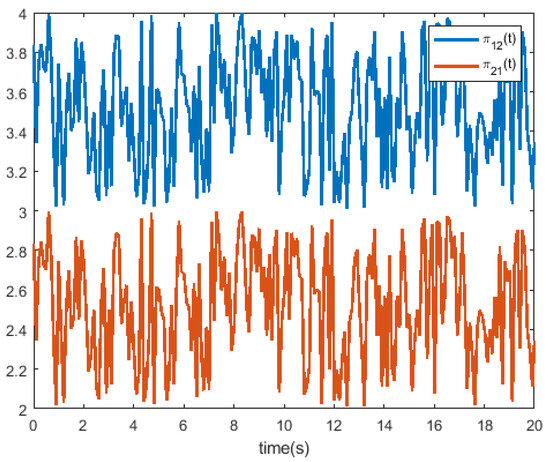
Figure 1. The responses of ${\pi }_{12}\left(t\right)$ and ${\pi }_{21}\left(t\right)$.

To simplify the notation, we define $F_r=F\left(r\left(t\right)\right)$, $f_{r\psi }=f_{\psi }\left(r\left(t\right)\right)$, and the same for $G_r$ with $g_{r\psi }$ being either 0 or 1. Additionally, in Equation (9), we establish the bounds $0\le {\underline{f}}_{r\psi }\le f_{r\psi }\le {\overline{f}}_{r\psi }\le 1$, where ${\underline{f}}_{r\psi }$ and ${\overline{f}}_{r\psi }$ are the lower and upper limits of $f_{r\psi }$, respectively. By introducing the matrices ${\underline{F}}_r=diag\left\{{\underline{f}}_{r\psi }\right\}$, ${\overline{F}}_r=diag\left\{{\overline{f}}_{r\psi }\right\}$, $F_{r0}=\frac{{\underline{F}}_r+{\overline{F}}_r}{2}$, and $F_{r1}=\frac{{\overline{F}}_r-{\underline{F}}_r}{2}$, we can express $F_r$ as a combination of $F_{r0}$ and $F_{r1}$ scaled by ${\sum }_r$, where ${\sum }_r=diag\{{\sigma }_{r1},{\sigma }_{r2},\dots ,{\sigma }_{rn}\}$ with $-1\le {\sigma }_{r\psi }\le 1$.

By incorporating (6) and (9), we introduce the following fuzzy FTC strategy. Under the sampled-data input, this controller is designed as follows:

Rule i: IF $\left\{{\lambda }_1\left(t_k\right)\mathrm{is}{\mathrm{M}}_1^{\mathrm{i}}\right\}$, $\left\{{\lambda }_2\left(t_k\right)\mathrm{is}{\mathrm{M}}_2^{\mathrm{i}}\right\}$,..., $\left\{{\lambda }_f\left(t_k\right)\mathrm{is}{\mathrm{M}}_{\mathrm{f}}^{\mathrm{i}}\right\}$, THEN

$$\begin{array}{c}\hfill u^f\left(t\right)=\sum _{j=1}^p{h}_j\left(\lambda \left(t_k\right)\right)\left\{F_r{K}_{rj}\sum _{l_1=1}^m\sum _{l_2=1}^m{\theta }_{l_1{l}_2}{L}_{l_2}y\left(t_k\right)+G_{r}v\left(t\right)\right\},t\in [t_k,t_{k+1})\end{array}$$

(14)

where $K_{rj}(j=1,2,\dots ,m)$ is the desired controller.

Combining (14) and (6), we can derive the following closed-loop system:

$$\begin{array}{c}\hfill \left\{\begin{array}{ccc}\dot{x}\left(t\right)\hfill & =\hfill & \sum _{i=1}^p\sum _{j=1}^p{h}_i\left(\lambda \left(t\right)\right)h_j\left(\lambda \left(t_k\right)\right)[A_{i}x\left(t\right)+B_i{G}_{r}v\left(t\right)+H_i\tilde{d}\left(t\right)\hfill \\ & & +B_i{F}_r{K}_{rj}\sum _{l_1=1}^m\sum _{l_2=1}^m{\theta }_{l_1{l}_2}{L}_{l_2}{C}_{i}x(t-\tau \left(t\right))]\hfill \\ y\left(t\right)\hfill & =\hfill & \sum _{i=1}^p\sum _{j=1}^p{h}_i\left(\lambda \left(t\right)\right)h_j\left(\lambda \left(t_k\right)\right)C_{i}x\left(t\right)\hfill \end{array}\right.\end{array}$$

(15)

Furthermore, by recognizing that

$$\begin{array}{c}\hfill B_i{F}_r{K}_{rj}\sum _{l_1=1}^m\sum _{l_2=1}^m{\theta }_{l_1{l}_2}{L}_{l_2}=B_i{F}_r{K}_{rj}{\mathcal{I}}^{T}qm(\mathsf{\Theta }⨂Iq)L{C}_{i}x(t-\tau \left(t\right))\end{array}$$

we can rewrite (15) as

$$\begin{array}{c}\hfill \left\{\begin{array}{ccc}\dot{x}\left(t\right)\hfill & =\hfill & \sum _{i=1}^p\sum _{j=1}^p{h}_i\left(\lambda \left(t\right)\right)h_j\left(\lambda \left(t_k\right)\right)[A_{i}x\left(t\right)\hfill \\ & & +B_i{F}_r{K}_{rj}{\mathcal{I}}_{qm}^T(\mathsf{\Theta }⨂I_q)L{C}_{i}x(t-\tau \left(t\right))\hfill \\ & & +B_i{G}_{r}v\left(t\right)+H_i\tilde{d}\left(t\right)]\hfill \\ y\left(t\right)\hfill & =\hfill & \sum _{i=1}^p\sum _{j=1}^p{h}_i\left(\lambda \left(t\right)\right)h_j\left(\lambda \left(t_k\right)\right)C_{i}x\left(t\right)\hfill \end{array}\right.\end{array}$$

(16)

where ${\mathcal{I}}_{qm}^T=\underset{m}{\underbrace{[I_q,I_q,\dots ,I_q]}}$ and $L={[L_1,L_2,\dots ,L_m]}^T.$

In this paper, our primary aim is to develop a fuzzy fault-tolerant controller with the goal of satisfying the following performance criteria:

(i) Provided with scalars $c_1>0,c_2>0,{\tau }_M>0,\overline{w}>0,T>0$, and a positive definite matrix $R>0$, we can conclude that system (16) exhibits finite-time stability and data boundedness (FTSDB) concerning the parameters $(c_1,c_2,{\tau }_M,\overline{w},T,H)$ if the following conditions hold:

$$\begin{array}{c}\hfill \underset{-{\tau }_M\le s\le 0}{sup}\mathcal{E}[x^T\left(s\right)Rx\left(s\right),{\dot{x}}^T\left(s\right)R\dot{x}\left(s\right)]\le c_1\Rightarrow \mathcal{E}\left[x^T\left(t\right)Rx\left(t\right)\right]<c_2,\forall t\in [0,T]\end{array}$$

(ii) For $T>0$ and $\gamma >0$, if the following condition is satisfied, then (16) meets the $H_{\infty }$ performance:

$$\begin{array}{c}\hfill {\int }_0^T{\gamma }^2{w}^T\left(s\right)w\left(s\right)-y^T\left(s\right)y\left(s\right)ds>0\end{array}$$

(17)

By defining w(s)$\triangleq {[v^T\left(s\right),{\tilde{d}}^T\left(s\right)]}^T$ and imposing the constraint ${\int }_0^T{w}^T\left(s\right)w\left(s\right)ds\le \overline{v}+\overline{d}\triangleq \overline{w}$, we devise a methodology that capitalizes on the recorded output from an individual sensor and its adjacent sensors. This approach yields a novel condition for maintaining system stability with the added constraint of $H_{\infty }$ performance. Additionally, we derive a method for designing controller gains to meet these requirements.

3. Main Result

To date, the Lyapunov stability analysis method has been extensively applied in the design of controllers for systems with delays, owing to its broad range of potential applications. In line with this approach, the primary findings of this paper have also been derived. To derive the FTC method, we will introduce two helpful preconditions.

Lemma 1 ([32]).

Given constants $\beta >\alpha >0$, $R>0$ and variable x: $[\alpha ,\beta ]\times {\mathbb{R}}^n\to {\mathbb{R}}^n$, one has

$$\begin{array}{c}\hfill (\beta -\alpha ){\int }_{\alpha }^{\beta }{x}^T\left(p\right)Rx\left(p\right)dp\ge {\int }_{\alpha }^{\beta }{x}^T\left(p\right)dpR{\int }_a^b{x}^T\left(p\right)dp\end{array}$$

Lemma 2 ([22]).

Given P, Q, and R, if there exists $\left|\right|Q\left|\right|\le 1$, then for $ϵ>0$, the following condition holds:

$$\begin{array}{c}\hfill {\left[PQR\right]}_s\le {ϵ}^{-1}P{P}^T+ϵR^{T}R\end{array}$$

Theorem 1.

Given scalar values ${\epsilon }_1$, ${\epsilon }_2$, $\alpha >0,\gamma >0,{\tau }_M>0,c_1>0$, and $H>0$, system (16) is exponential stability in the mean-square sense and can be characterized as FTSDB concerning the parameters $(c_1,c_2,{\tau }_M,\overline{w},\widehat{d},T,H)$ and satisfies the $H_{\infty }$ performance criterion if there exist scalar values $c_2>0$, ${\rho }_1$, $P_r^l>0$, $Q>0$, $R>0$, $W>0$, $Z_{ij}>0$, and matrices $U_1$, $U_2$, such that

$$\begin{array}{c}\hfill \left[\begin{array}{cc}\frac{1}{2}({\left[{\mathsf{\Omega }}_{ij}^{ls}\left(1\right)\right]}_s+{\left[{\mathsf{\Omega }}_{ij}^{sl}\left(1\right)\right]}_s)+X_{ij}{Z}_{ij}{X}_{ij}^T& Y_{ij}\\ \ast & -Z_{ij}\end{array}\right]<0\end{array}$$

(18)

$$\begin{array}{c}\hfill \left[\begin{array}{cc}\frac{1}{2}({\left[{\mathsf{\Omega }}_{ij}^{ls}\left(e^{0.5\alpha {\tau }_M}\right)\right]}_s+{\left[{\mathsf{\Omega }}_{ij}^{sl}\left(e^{0.5\alpha {\tau }_M}\right)\right]}_s)+X_{ij}{Z}_{ij}{X}_{ij}^T& Y_{ij}\\ \ast & -Z_{ij}\end{array}\right]<0\end{array}$$

(19)

$$\begin{array}{c}\hfill e^{\alpha T}\{c_1[{\mu }_1+{\mu }_2{\mu }^{\prime }]+2(c_1{\mu }_3+\widehat{d}){\mu }^{″}+{\gamma }^2\overline{w}\}<c_{2}m{u}_0\end{array}$$

(20)

where ${\mathsf{\Omega }}_{ij}^{sl}\left(e^{0.5\alpha \tau \left(t\right)}\right)={\left[{\phi }^{sl}\right]}_{5\times 5}(1\le i\le j\le p)$ and

$$\begin{array}{ccc}\hfill {\mu }_0& =& {\mu }_{min}(\frac{1}{{\rho }_1^2}{\tilde{P}}_r^l),{\mu }_1={\mu }_{max}({\tilde{P}}_r^l),{\mu }_2={\mu }_{max}\left(\tilde{Q}\right),{\mu }_3={\mu }_{max}\left(\tilde{R}\right)\hfill \end{array}$$

(21)

$$\begin{array}{ccc}\hfill {\tilde{P}}_r^l& =& {\rho }_1^2{H}^{-\frac{1}{2}}{P}_r^l{H}^{-\frac{1}{2}},\tilde{Q}={\rho }_1^2{H}^{-\frac{1}{2}}Q{H}^{-\frac{1}{2}},\tilde{R}={\rho }_1^2{H}^{-\frac{1}{2}}{A}_{i}R{A}_i{H}^{-\frac{1}{2}}\hfill \end{array}$$

(22)

$$\begin{array}{ccc}\hfill {\mu }^{\prime }& =& \frac{e^{\alpha }{\tau }_M-1}{\alpha },{\mu }^{″}=\frac{e^{\alpha }{\tau }_M}{{\alpha }^2}-\frac{1}{{\alpha }^2}-\frac{{\tau }_M}{{\alpha }^2}\hfill \end{array}$$

(23)

$$\begin{array}{ccc}\hfill {\phi }_{11}^{sl}& =& Q-\alpha P_r^l-\frac{R}{{\tau }_M}-\frac{{\pi }^2}{4{\tau }_M^2}W+C_i^T{C}_i+{\epsilon }_1{U}_1^T{A}_i+{\epsilon }_1{A}_i^T{U}_1\hfill \end{array}$$

(24)

$$\begin{array}{ccc}& & +\sum _{h=1}^N{\pi }_{rh}^s{P}_h^l+\sum _{n=1}^{Z-1}(\pm v_n)(P_r^Z-P_r^n)\hfill \end{array}$$

(25)

$$\begin{array}{ccc}\hfill {\phi }_{12}& =& P_r^l-{\epsilon }_1{U}_1^T+{\epsilon }_2{A}_i^T{U}_2\hfill \end{array}$$

(26)

$$\begin{array}{ccc}\hfill {\phi }_{13}& =& \frac{R}{{\tau }_M}+e^{0.5\alpha \tau \left(t\right)}\frac{{\pi }^2}{4{\tau }_M^2}W+{\epsilon }_1{U}_1^T{B}_i{F}_r{K}_{rj}{\mathcal{I}}_{qm}^T(\mathsf{\Theta }⨂I_q)L{C}_i\hfill \end{array}$$

(27)

$$\begin{array}{ccc}\hfill {\phi }_{15}& =& {\epsilon }_1{U}_1^T{H}_i+{\epsilon }_1{U}_1^T{B}_i{G}_r\hfill \end{array}$$

(28)

$$\begin{array}{ccc}\hfill {\phi }_{22}& =& {\tau }_{M}R-{\epsilon }_2{U}_2^T-{\epsilon }_2{U}_2+W\hfill \end{array}$$

(29)

$$\begin{array}{ccc}\hfill {\phi }_{23}& =& {\epsilon }_2{U}_2^T{B}_i{F}_r{K}_{rj}{\mathcal{I}}_{qm}^T(\mathsf{\Theta }⨂I_q)L{C}_i\hfill \end{array}$$

(30)

$$\begin{array}{ccc}\hfill {\phi }_{25}& =& {\epsilon }_2{U}_2^T{H}_i+{\epsilon }_2{U}_2^T{B}_i{G}_r\hfill \end{array}$$

(31)

$$\begin{array}{ccc}\hfill {\phi }_{33}& =& -\frac{2}{{\tau }_M}R-e^{\alpha \tau \left(t\right)}\frac{{\pi }^2}{4{\tau }_M^2}W,{\phi }_{34}=\frac{1}{{\tau }_M}R\hfill \end{array}$$

(32)

$$\begin{array}{ccc}\hfill {\phi }_{44}& =& -e^{\alpha {\tau }_M}Q-\frac{1}{{\tau }_M}R,{\phi }_{55}=-{\gamma }^2{I}_n\hfill \end{array}$$

(33)

$$\begin{array}{ccc}\hfill X_{ij}& =& {[\frac{{\epsilon }_1{(B_i+B_j)}^T}{2}{U}_1,\frac{{\epsilon }_2{(B_i+B_j)}^T}{2}{U}_2,0]}^T\underset{r}{\underbrace{[I,I,\dots ,I]}}\hfill \end{array}$$

(34)

$$\begin{array}{ccc}\hfill Y_{ij}& =& [0,I,0][\frac{(C_i+C_j)}{2}{L}^T{(\mathsf{\Theta }⨂I_q)}^T{\mathcal{I}}_{qm}{K}_{r1}^T{F}_r^T,\dots ,\frac{(C_i+C_j)}{2}{L}^T{(\mathsf{\Theta }⨂I_q)}^T{\mathcal{I}}_{qm}{K}_{rp}^T{F}_r^T]\hfill \end{array}$$

(35)

Proof. 

Let us formulate the nonhomogeneous Lyapunov functional as follows:

$$\begin{array}{c}\hfill \mathfrak{V}(t,r_t)={\mathfrak{V}}_1(t,r_t)+{\mathfrak{V}}_2(t,r_t)+{\mathfrak{V}}_3(t,r_t)+{\mathfrak{V}}_4(t,r_t)\end{array}$$

(36)

where

$$\begin{array}{ccc}\hfill {\mathfrak{V}}_1(t,r_t)& =& x^T\left(t\right)P_r\left(t\right)x\left(t\right)\hfill \\ \hfill {\mathfrak{V}}_2(t,r_t)& =& {\int }_{t-{\tau }_M}^t{e}^{\alpha (t-p)}{x}^T\left(p\right)Qx\left(p\right)dp\hfill \\ \hfill {\mathfrak{V}}_3(t,r_t)& =& {\int }_{t-{\tau }_M}^t{\int }_{\beta }^t{e}^{\alpha (t-p)}{\dot{x}}^T\left(p\right)R\dot{x}\left(p\right)dpd\beta \hfill \\ \hfill {\mathfrak{V}}_4(t,r_t)& =& {\int }_{t_k}^t\frac{d}{dp}{\left(e^{0.5\alpha (t-p)}x\left(p\right)\right)}^{T}W(e^{0.5\alpha (t-p)}x\left(p\right))dp\hfill \\ & & -\frac{{\pi }^2}{4{\tau }_M^2}{\int }_{t_k}^t{(e^{0.5\alpha (t-p)}x\left(p\right)-e^{0.5\alpha (t-t_k)}x\left(t_k\right))}^T\hfill \\ & \times & W(e^{0.5\alpha (t-p)}x\left(p\right)-e^{0.5\alpha (t-t_k)}x\left(t_k\right))dp\hfill \end{array}$$

Let $\mathfrak{L}$ be the weak infinitesimal generator. Along the nonhomogenous Markov distribution, we have

$$\begin{array}{c}\hfill \mathfrak{L}\mathfrak{V}(t,r_t)=\underset{\mathsf{\Delta }\to 0}{lim}\frac{\mathcal{E}\left\{\mathfrak{V}(x_{t+\mathsf{\Delta }},t+\mathsf{\Delta },r_{t+\mathsf{\Delta }})S\right|r_t=r\}-\mathfrak{V}(t,r)}{\mathsf{\Delta }},r\in S\end{array}$$

When calculating $\mathfrak{L}\mathfrak{V}(t,r_t)$ along the closed-loop system given in (16), we obtain the following result:

$$\begin{array}{ccc}\hfill \mathfrak{L}{\mathfrak{V}}_1(t,r_t)& =& 2x^T\left(t\right)P_r\left(t\right)\dot{x}\left(t\right)+x^T\left(t\right)[\sum _{h=1}^N{\pi }_{rh}\left(t\right)P_r\left(t\right)]x\left(t\right)+x^T\left(t\right){\dot{P}}_r\left(t\right)x\left(t\right)\hfill \\ \hfill \mathfrak{L}{\mathfrak{V}}_2(t,r_t)& =& \alpha {\mathfrak{V}}_2(t,r_t)+x^T\left(t\right)Qx\left(t\right)-e^{\alpha {\tau }_M}{x}^T(t-{\tau }_M)Q(t-{\tau }_M)\hfill \\ & & +{\tau }_M{\dot{x}}^T\left(t\right)R\dot{x}\left(t\right)-e^{\alpha {\tau }_M}{\dot{x}}^T\left(t\right)R\dot{x}\left(t\right)-{\int }_{t-{\tau }_M}^t{e}^{\alpha (t-s)}{\dot{x}}^T\left(s\right)R\dot{x}\left(s\right)ds\hfill \\ & & +{\dot{x}}^T\left(t\right)W\dot{x}\left(t\right)-\frac{{\pi }^2}{4{\tau }_M^2}{[x\left(t\right)-e^{0.5\alpha (t-t_k)}x\left(t_k\right)]}^{T}W[x\left(t\right)-e^{0.5\alpha (t-t_k)}x\left(t_k\right)].\hfill \end{array}$$

Building upon Lemma 1, we derive a lower bound for ${\int }_{t-{\tau }_M}^t{\dot{x}}^T\left(p\right)R\dot{x}\left(p\right)dp$ as follows:

$$\begin{array}{ccc}\hfill {\int }_{t-{\tau }_M}^t{\dot{x}}^T\left(p\right)R\dot{x}\left(p\right)dp& \ge & \frac{1}{{\tau }_M}{[x\left(t\right)-x(t-\tau \left(t\right))]}^{T}R[x\left(t\right)-x(t-\tau \left(t\right))]\hfill \\ & & +\frac{1}{{\tau }_M}{[x(t-\tau \left(t\right))-x(t-{\tau }_M)]}^T\hfill \\ & \times & R[x(t-\tau \left(t\right))-x(t-{\tau }_M)]\hfill \end{array}$$

(37)

For $U_1$, $U_2$ and any free parameters ${\epsilon }_1$, ${\epsilon }_2$, one has

$$\begin{array}{ccc}\hfill & & 2\{\dot{x}\left(t\right)-\sum _{i=1}^p\sum _{i=1}^p{h}_i\left(\lambda \left(t\right)\right)h_j\left(\lambda \left(t_k\right)\right)[A_{i}x\left(t\right)\hfill \\ & & +B_i{F}_r{K}_{rj}{\mathcal{I}}_{qm}^T(\mathsf{\Theta }⨂I_q)L{C}_{i}x\left(t_k\right)+B_i{G}_{r}v\left(t\right)+H_i\tilde{d}\left(t\right)\left]\right\}{U}^T\zeta \left(t\right)=0\hfill \end{array}$$

(38)

where

$$\begin{array}{ccc}\hfill U& =& {[{\epsilon }_1{U}_1,{\epsilon }_2{U}_2,0,0,0]}^T\hfill \\ \hfill \zeta & =& {[x^T\left(t\right),{\dot{x}}^T\left(t\right),x^T(t-\tau \left(t\right)),x^T(t-{\tau }_M),w^T\left(t\right)]}^T\hfill \end{array}$$

Together with ${\mathfrak{V}}_3(t,r_t)$ and ${\mathfrak{V}}_4(t,r_t)$, it yields

$$\begin{array}{ccc}& & \mathfrak{L}\mathfrak{V}(t,r_t)-\alpha V(t,r_t)-{\gamma }^2{w}^T\left(t\right)w\left(t\right)+y^T\left(t\right)y\left(t\right)\hfill \\ & =& \mathfrak{L}\mathfrak{V}(t,r_t)-\alpha V(t,r_t)-{\gamma }^2{w}^T\left(t\right)w\left(t\right)+y^T\left(t\right)y\left(t\right)\hfill \\ & -& 2{\zeta }^T\left(t\right)U\{\dot{x}\left(t\right)-\sum _{i=1}^p\sum _{j=1}^p{h}_i\left(\lambda \left(t\right)\right)h_j\left(\lambda \left(t_k\right)\right)\hfill \\ & \times & \left[A_{i}x\left(t\right)+B_i{F}_r{K}_{rj}{\mathcal{I}}_{qm}^T(\mathsf{\Theta }⨂I_q)L{C}_{i}x\left(t_k\right)+B_i{G}_{r}v\left(t\right)+H_i\tilde{d}\left(t\right)\right]\}\hfill \\ & \le & \sum _{i=1}^p\sum _{j=1}^p{h}_i\left(\lambda \left(t\right)\right)h_j\left(\lambda \left(t_k\right)\right){\zeta }^T\left(t\right){\mathsf{\Omega }}_{ij}^{ls}\zeta \left(t\right)\hfill \end{array}$$

Let ${ϵ}_j\left(\lambda \left(t\right)\right)=h_j\left(\lambda \left(t_k\right)\right)-h_j\left(\lambda \left(t\right)\right),$${\sum }_{k=1}^pϵ\left(\lambda \left(t_k\right)\right)=0$. One has

$$\begin{array}{ccc}& & \sum _{i=1}^p\sum _{i=1}^m{h}_i\left(\lambda \left(t\right)\right)\sum _{j=1}^m{h}_j\left(\lambda \left(t_k\right)\right){\zeta }^T\left(t\right){\mathsf{\Omega }}_{ij}\zeta \left(t\right)\hfill \\ & =& \sum _{i=1}^p\sum _{i=1}^m{h}_i\left(\lambda \left(t\right)\right)\sum _{j=1}^m{h}_j\left(\lambda \left(t_k\right)\right){\zeta }^T\left(t\right)\left[\frac{{\mathsf{\Omega }}_{ij}+{\mathsf{\Omega }}_{ji}}{2}+\sum _{k=1}^p{ϵ}_k\left(\lambda \left(t\right)\right)\frac{{\mathsf{\Omega }}_{ik}+{\mathsf{\Omega }}_{jk}}{2}\right]\zeta \left(t\right)\hfill \\ & & \sum _{k=1}^p{ϵ}_k\left(\lambda \left(t\right)\right)\frac{{\mathsf{\Omega }}_{ik}+{\mathsf{\Omega }}_{jk}}{2}\hfill \\ & =& \sum _{k=1}^p{ϵ}_k\left(\lambda \left(t\right)\right)\left[\begin{array}{ccc}0& U_1^T\frac{B_i+B_j}{2}{F}_r{K}_{rk}{\mathcal{I}}_{qm}^T(\mathsf{\Theta }⨂I_q)L\frac{C_i+C_j}{2}& 0\\ 0& U_2^T\frac{B_i+B_j}{2}{F}_r{K}_{rk}{\mathcal{I}}_{qm}^T(\mathsf{\Theta }⨂I_q)L\frac{C_i+C_j}{2}& 0\\ 0& 0& 0\end{array}\right]\hfill \\ & =& \{\left[\begin{array}{c}{U}_1^T\frac{B_i+B_j}{2}\\ U_2^T\frac{B_i+B_j}{2}\\ 0\end{array}\right]\underset{r}{\underbrace{\left[\begin{array}{cccc}I& I& \cdots & I\end{array}\right]}}\mathsf{\Gamma }\left(\lambda \left(t\right)\right)\hfill \\ & \times & \left[\begin{array}{c}{F}_r{K}_{r1}{\mathcal{I}}_{qm}^T(\mathsf{\Theta }⨂I_q)L\frac{C_i+C_j}{2}\\ F_r{K}_{r2}{\mathcal{I}}_{qm}^T(\mathsf{\Theta }⨂I_q)L\frac{C_i+C_j}{2}\\ \cdots \\ F_r{K}_{rp}{\mathcal{I}}_{qm}^T(\mathsf{\Theta }⨂I_q)L\frac{C_i+C_j}{2}\end{array}\right]\left[\begin{array}{ccc}0& I& 0\end{array}\right]\}\hfill \\ & \le & X_{ij}{Z}_{ij}{X}_{ij}^T+Y_{ij}{Z}_{ij}^{-1}{Y}_{ij}^T\triangleq {\mathsf{\Lambda }}_{ij}\hfill \end{array}$$

where $\mathsf{\Gamma }\left(\lambda \left(t\right)\right)=diag\{{ϵ}_1\left(\lambda \left(t\right)\right),{ϵ}_2\left(\lambda \left(t\right)\right),\dots ,{ϵ}_p\left(\lambda \left(t\right)\right)\}$.

Note that

$$\begin{array}{c}\hfill P_r\left(t\right)=\sum _{l=1}^Z{\alpha }_l\left(t\right)P_r^l,\end{array}$$

(39)

We have ${\dot{P}}_r\left(t\right)={\sum }_{l=1}^Z{\dot{\alpha }}_l\left(t\right)P_r^l.$ Consider that

$${\dot{\alpha }}_Z\left(t\right)=-\sum _{l=1}^{Z-1}{\dot{\alpha }}_l\left(t\right),$$

Thus, we obtain

$$\begin{array}{c}\hfill {\dot{P}}_r\left(t\right)=\sum _{l=1}^Z{\dot{\alpha }}_l\left(t\right)P_r^l=\sum _{n=1}^{Z-1}{\dot{\alpha }}_n\left(t\right)(P_r^n-P_r^Z).\end{array}$$

(40)

It is important to note that ${\dot{\alpha }}_n\left(t\right)$ (which belongs to the interval $[-v_n,v_n]$) can be considered either as an upper or lower bound. Thus, ${\sum }_{n=1}^{Z-1}(\pm v_n)(P_r^n-P_r^Z)\ge (\le )0$ can lead to the conclusion that ${\dot{P}}_r\left(t\right)={\sum }_{n=1}^{Z-1}{\dot{\alpha }}_n\left(t\right)(P_r^n-P_r^Z)\ge (\le )0$.

Due to the presence of the nonhomogeneous terms ${\psi }_{13}$ and ${\psi }_{33}$, it should be noted that the inequality in Equation (18) is infinite and nonlinear in nature. Define $y\left(t\right)=e^{{0.5}^{\alpha \tau \left(t\right)}}$. Since $1\le y\left(t\right)\le e^{0.5\alpha {\tau }_M}$, if the matrices ${\mathsf{\Omega }}_{ij}\left(1\right)$ and ${\mathsf{\Omega }}_{ij}\left(e^{0.5\alpha {\tau }_M}\right)$ satisfy the conditions (18) and (19), one has

$$\begin{array}{c}\hfill \sum _{i=1}^r\sum _{j=1}^r{h}_i\left(\lambda \left(t\right)\right)h_j\left(\lambda \left(t_k\right)\right){\xi }^T\left[\sum _{l=1}^Z{\alpha }_l^2{\mathsf{\Omega }}_{ij}^{ll}+\sum _{l=1}^{Z-1}\sum _{s=l+1}^Z{\alpha }_l\left(t\right){\alpha }_s\left(t\right)({\mathsf{\Omega }}_{ij}^{ls}+{\mathsf{\Omega }}_{ij}^{sl})\right]\xi <0\end{array}$$

(41)

Considering the inequality $y^T\left(t\right)y\left(t\right)\ge 0$, we have

$$\begin{array}{c}\hfill \mathfrak{L}\mathfrak{V}(t,r_t)<\alpha \mathfrak{V}(t,r_t)+{\gamma }^2{w}^T\left(t\right)w\left(t\right)\end{array}$$

Considering the interval $(t,t_k)$, one has

$$\begin{array}{ccc}\hfill \mathcal{E}\left[\mathfrak{V}(t,r_t)\right]& <& \mathcal{E}\left[\mathfrak{V}(t_k,r_t)\right]e^{\alpha (t-t_k)}+{\int }_{t_k}^t{\gamma }^2{w}^T\left(p\right)w\left(p\right)dp\hfill \\ & <& \mathcal{E}\left[\mathfrak{V}(t_k,r_t)\right]e^{\alpha (t-t_k)}+{\int }_{t_k}^t{e}^{\alpha (t-s)}{\gamma }^2{w}^T\left(p\right)w\left(p\right)dp.\hfill \end{array}$$

Moving forward, we will establish an upper bound for $V(t_0,r_0)$, taking into account the continuity property ${lim}_{t\to t_k^{-}}V(t,r_t)=V(t_k,r_{t_k})$

$$\begin{array}{ccc}\hfill \mathcal{E}\left[\mathfrak{V}(t,r_t)\right]& <& \mathcal{E}\left[\mathfrak{V}(t_k^{-},r_t)\right]e^{\alpha (t-t_k)}+{\int }_{t_k}^t{e}^{\alpha (t-p)}{\gamma }^2{w}^T\left(p\right)w\left(p\right)dp\hfill \\ & <& \left\{\mathcal{E}\left[\mathfrak{V}(t_{k-1},r_t)\right]e^{\alpha (t_k^{-}-t_{k-1})}+{\int }_{t_{k-1}}^{t_k^{-}}{e}^{\alpha (t_k^{-}-p)}{\gamma }^2{w}^T\left(s\right)w\left(s\right)ds\right\}{e}^{\alpha (t-t_k)}\hfill \\ & & +{\int }_{t_k}^t{e}^{\alpha (t-s)}{\gamma }^2{w}^T\left(s\right)w\left(s\right)ds\hfill \\ & =& \mathcal{E}\left[\mathfrak{V}(t_{k-1},r_t)\right]e^{\alpha (t-t_{k-1})}+{\int }_{t_{k-1}}^t{e}^{\alpha (t-p)}{\gamma }^2{w}^T\left(p\right)w\left(p\right)dp\hfill \\ & & ⋮\hfill \\ & <& \mathcal{E}\left[\mathfrak{V}(t_0,r_t)\right]e^{\alpha (t-t_0)}+{\int }_{t_0}^t{e}^{\alpha (t-p)}{\gamma }^2{w}^T\left(p\right)w\left(p\right)dp\hfill \end{array}$$

Considering that the initial sampling instant $t_0$ may not coincide with 0, let us address $\mathfrak{V}(t_0,r_0)$ by accounting for the following: When t lies within the interval $[-{\tau }_M,t_0]$, we set $u\left(t\right)=0$. Consequently, based on the following condition, we can derive the nonlinear spacecraft dynamics

$$\begin{array}{c}\hfill \dot{x}\left(t\right)=A\left(t\right)x\left(t\right)+\widehat{d}\left(t\right),A\left(t\right)=\sum _{i=1}^r{h}_i\left(\lambda \left(t\right)\right)A_i,t\in [-{\tau }_M,t_0]\end{array}$$

(42)

which means

$$\begin{array}{c}\hfill x\left(t\right)=e^{{\int }_0^{t}A\left(p\right)dp}x\left(0\right)+e^{{\int }_0^{t}A\left(p\right)dp}{\int }_0^t{e}^{-{\int }_0^{s}A\left(\beta \right)d\beta }\widehat{d}\left(p\right)dp.\end{array}$$

(43)

Based the norm space, it yields

$$\begin{array}{c}\hfill \left|\right|x\left(t\right)\left|\right|=\left|\right|e^{{\int }_0^{t}A\left(p\right)dp}||\dot{|}|x\left(0\right)\left|\right|+\left|\right|e^{{\int }_0^{t}A\left(p\right)dp}||\dot{|}|{\int }_0^t{e}^{-{\int }_0^{p}A\left(\beta \right)d\beta }\widehat{d}\left(p\right)dp\left|\right|.\end{array}$$

It is clear that there are constants ${\varrho }_1$, ${\varrho }_2$, and ${\varrho }_3$ such that

$$\begin{array}{ccc}\hfill {\varrho }_2& \ge & \left|\right|e^{{\int }_0^{t}A\left(p\right)dp}||\dot{|}|{\int }_0^t{e}^{-{\int }_0^{s}A\left(\beta \right)d\beta }\widehat{d}\left(p\right)dp\left|\right|,{\varrho }_3\ge \left|\right|e^{{\int }_0^{t}A\left(p\right)dp}\left|\right|,\hfill \\ \hfill \left|\right|x\left(t\right)\left|\right|& \le & {\varrho }_3\left|\right|x\left(0\right)\left|\right|+{\varrho }_2={\varrho }_1\left|\right|x\left(0\right)\left|\right|.\hfill \end{array}$$

For $H>0$, one has

$$\begin{array}{c}\hfill x^T\left(t\right)Hx\left(t\right)\le {\varrho }_1^2{x}^T\left(0\right)Hx\left(0\right).\end{array}$$

(44)

which can be further deduced as

$$\begin{array}{ccc}\hfill \mathfrak{V}(t_0,r_{t_0})& =& x^T\left(t_0\right)P_{a}x\left(t_0\right)+{\int }_{t_0-{\tau }_M}^{t_0}{e}^{\alpha (t_0-p)}{x}^T\left(p\right)Qx\left(p\right)dp\hfill \\ & & +{\int }_{t_0-{\tau }_M}^{t_0}{\int }_{\beta }^{t_0}{e}^{\alpha (t_0-p)}{\dot{x}}^T\left(p\right)R\dot{x}\left(p\right)dpd\beta \hfill \end{array}$$

Set $t=t_0$ in (44), and let $x_0$ be known. It is not difficult to see that

$$\begin{array}{ccc}\hfill \mathfrak{V}(t_0,r_{t_0})& \le & {\psi }_1{x}^T\left(0\right)Hx\left(0\right)+{\int }_{t_0-{\tau }_M}^{t_0}{e}^{\alpha (t_0-p)}{\psi }_2{x}^T\left(0\right)Hx\left(0\right)dp\hfill \\ & & +{\int }_{t_0-{\tau }_M}^{t_0}{\int }_{\beta }^{t_0}{e}^{\alpha (t_0-p)}{\dot{x}}^T\left(s\right)R\dot{x}\left(s\right)dpd\beta \hfill \end{array}$$

It is obtained from (42) that

$$\begin{array}{ccc}\hfill {\dot{x}}^T\left(p\right)R\dot{x}\left(p\right)& =& {\left[A\left(p\right)x\left(p\right)+\widehat{d}\left(p\right)\right]}^{T}R\left[A\left(p\right)x\left(p\right)+\widehat{d}\left(p\right)\right]\hfill \\ & \le & 2{\left[A\left(p\right)x\left(p\right)\right]}^{T}R\left[A\left(p\right)x\left(p\right)\right]+2{\widehat{d}}^T\left(p\right)R\widehat{d}\left(p\right)\hfill \end{array}$$

which can further deduce

$$\begin{array}{ccc}\hfill \mathfrak{V}(t_0,r_{t_0})& \le & {\psi }_1{x}^T\left(0\right)Hx\left(0\right)+{\int }_{t_0-{\tau }_M}^{t_0}{e}^{\alpha (t_0-s)}{\psi }_2{x}^T\left(0\right)Hx\left(0\right)dp\hfill \\ & & +2{\int }_{t_0-{\tau }_M}^{t_0}{\int }_{\beta }^{t_0}{e}^{\alpha (t_0-p)}[x^T\left(p\right)A^T\left(p\right)RA\left(p\right)x\left(p\right)\hfill \\ & & +{\widehat{d}}^T\left(p\right)+{\widehat{d}}^T\left(p\right)R\widehat{d}\left(p\right)]dpd\beta \hfill \end{array}$$

Let $su{p}_{-{\tau }_M\le p\le 0}\left[x^T\left(p\right)Hx\left(p\right)\right]=c_1$, ${\widehat{d}}^T\left(p\right)R\widehat{d}\left(p\right)\le \widehat{d}$. It is easy to see that

$$\begin{array}{ccc}\hfill \mathfrak{V}(t_0,r_{t_0})& \le & {\psi }_1{c}_1+{\psi }_2{\int }_{t_0-{\tau }_M}^{t_0}{e}^{\alpha (t_0-p)}{c}_{1}dp\hfill \\ & & +2{\int }_{t_0-{\tau }_M}^{t_0}{\int }_{\beta }^{t_0}{e}^{\alpha (t_0-p)}({\psi }_3{c}_1+\widehat{d})dpd\beta \hfill \\ & =& c_1\left[{\psi }_1+{\psi }_2\frac{1}{\alpha }(e^{\alpha {\tau }_M}-1)\right]+2(c_1{\psi }_3+\widehat{d})\left(\frac{1}{{\alpha }^2}{e}^{\alpha {\tau }_M}-\frac{1}{{\alpha }^2}-\frac{1}{\alpha }{\tau }_M\right)\hfill \end{array}$$

Due to $\mathfrak{V}(t,r_t)\ge {\psi }_0{x}^T\left(t\right)Hx\left(t\right)$, one has

$$\begin{array}{ccc}\hfill {\psi }_0{x}^T\left(t\right)Hx\left(t\right)& <& e^{\alpha t}[\mathfrak{V}(t_0,r_{t_0})+{\gamma }^2\overline{w}]\hfill \\ & <& e^{\alpha T}\left\{c_1[{\psi }_1+{\psi }_2{\psi }^{\prime }]+2(c_1{\psi }_3+\widehat{d}){\psi }^{″}+{\gamma }^2\overline{w}\right\}<{\psi }_0{c}_2\hfill \end{array}$$

Since $\dot{\mathfrak{V}}(t,r_t)-\alpha V(t,r_t)-{\gamma }^2{w}^T\left(t\right)w\left(t\right)+y^T\left(t\right)y\left(t\right)<0$, it yields

$$\begin{array}{c}\hfill \mathfrak{V}(t,r_t)<e^{\alpha (t-t_0)}\mathfrak{V}(t_0,r_{t_0})+e^{\alpha t}{\int }_{t_0}^t({\gamma }^2{w}^T\left(p\right)w\left(p\right)-y^T\left(p\right)y\left(p\right))dp\end{array}$$

Under the initial condition, it yields

$$\begin{array}{c}\hfill \mathfrak{V}(t_0^{+},r_{t_0^{+}})<{\int }_{t_0}^{t_0^{+}}({\gamma }^2{w}^T\left(p\right)w\left(p\right)dp-y^T\left(p\right)y\left(p\right))dp\end{array}$$

From $\mathfrak{V}(t,r_t)>0$, it yields

$$\begin{array}{c}\hfill {\gamma }^2{w}^T\left(t\right)w\left(t\right)-y^T\left(t\right)y\left(t\right)>0\\ \hfill {\int }_0^T({\gamma }^2{w}^T\left(p\right)w\left(p\right)-y^T\left(p\right)y\left(p\right))dp>0\end{array}$$

This completes the proof. □

Remark 4.

In this research, the inclusion of the term $x^T\left(t\right)P_r\left(t\right)x\left(t\right)$ within ${\mathfrak{V}}_1(t,r_t)$ holds pivotal importance as it facilitates the integration of information pertaining to the nonhomogeneous Markov process. This augmentation significantly enhances the realism of our findings when compared to the existing literature. It is noteworthy that the transformation presented in Equation (40) plays a critical role in effectively managing the derivative of ${\mathfrak{V}}_1(t,r_t)$. Additionally, the introduction of boundary values denoted as $v_n$ serves to transform the non-feasible derivative $\dot{P_r}\left(t\right)$ into more tractable finite values.

It is noted that Theorem 1 is not easy to settle due to the presence of nonlinearity. In the following, a feasible condition to reach the finite-time controller will be given.

Theorem 2.

For any ${\epsilon }_1$, ${\epsilon }_2$ and positive constants α, γ, ${\tau }_M$, $c_1$, ${\eta }_1$, ${\eta }_2$, ${\eta }_3$, T, any matrix $H>0$, we can establish the existence of positive scalars $c_2$, ${\mu }_1$, ${\mu }_2$, ${\mu }_3$, ${\overline{P}}_r^l>0$, $\overline{Q}>0$, $\overline{R}>0$, $\overline{W}>0$, $Z_{ij}>0$, and any matrices $K_{rj}$, $\overline{U}$, for $r\in S$ such that

$$\begin{array}{ccc}\hfill \left[\begin{array}{cc}\frac{{\overline{\mathsf{\Omega }}}_{ij}^{ls}+{\overline{\mathsf{\Omega }}}_{ji}^{ls}+{\overline{\mathsf{\Omega }}}_{ij}^{sl}+{\overline{\mathsf{\Omega }}}_{ji}^{sl}}{2}+{\overline{X}}_{ij}{Z}_{ij}{\overline{X}}_{ij}^T& {\overline{Y}}_{ij}\\ \ast & -Z_{ij}\end{array}\right]& <& 0\hfill \end{array}$$

(45)

$$\begin{array}{ccc}\hfill \left[\begin{array}{cc}-{\overline{P}}_r^l& {\overline{U}}^{T}H\\ \ast & -H\end{array}\right]& <& 0\hfill \end{array}$$

(46)

$$\begin{array}{ccc}\hfill \left[\begin{array}{cc}{\overline{P}}_r^l-({\eta }_1\overline{U}+{\eta }_1{\overline{U}}^T)& I\\ \ast & -\frac{{\mu }_1}{{\eta }_1^2}H\end{array}\right]& <& 0\hfill \end{array}$$

(47)

$$\begin{array}{ccc}\hfill \left[\begin{array}{cc}\overline{Q}-({\eta }_2\overline{U}+{\eta }_2{\overline{U}}^T)& I\\ \ast & -\frac{{\mu }_2}{{\eta }_2^2}H\end{array}\right]& <& 0\hfill \end{array}$$

(48)

$$\begin{array}{ccc}\hfill \left[\begin{array}{cc}\overline{R}-({\eta }_3\overline{U}+{\eta }_3{\overline{U}}^T)& I\\ \ast & -\frac{{\mu }_3}{{\eta }_3^2}H\end{array}\right]& <& 0\hfill \end{array}$$

(49)

$$\begin{array}{ccc}\hfill c_1{\mu }_1+c_1{\mu }_2{\psi }^{\prime }+2(c_1{\mu }_3+\widehat{d}){\psi }^{″}+{\gamma }^2\overline{w}& <& c_2{e}^{-\alpha T}\hfill \end{array}$$

(50)

where ${\psi }^{\prime }\left(\alpha \right)=\frac{e^{\alpha {\tau }_M}-1}{\alpha }$, ${\psi }^{″}\left(\alpha \right)=\frac{1}{{\alpha }^2}{e}^{\alpha {\tau }_M}-\frac{1}{{\alpha }^2}-\frac{1}{\alpha }{\tau }_M$, symmetric matrix ${\overline{\mathsf{\Omega }}}_{ij}={\left[{\overline{\varphi }}^{sl}\right]}_{5\times 5}$

$$\begin{array}{ccc}\hfill {\overline{\varphi }}_{11}^{sl}& =& \overline{Q}-\alpha {\overline{P}}_r^l-\frac{1}{{\tau }_M}\overline{R}-\frac{{\pi }^2}{4{\tau }_M^2}\overline{W}+{\epsilon }_1^2{\overline{U}}^T{C}_i^T{C}_i\overline{U}+{\epsilon }_1{\overline{A}}_i\overline{U}+{\epsilon }_1{\overline{U}}^T{\overline{A}}_i^T\hfill \\ & & +\sum _{b=1}^N{\pi }_{rh}^s{\overline{P}}_h^l+\sum _{n=1}^{Z-1}(\pm v_n)(P_r^Z-P_r^n),{\overline{\varphi }}_{12}={\overline{P}}_r^l-{\epsilon }_1\overline{U}+{\epsilon }_2{\overline{U}}^T{\overline{A}}_i^T\hfill \\ \hfill {\overline{\varphi }}_{13}& =& \frac{1}{{\tau }_M}\overline{R}+e^{0.5\alpha \tau \left(t\right)}\frac{{\pi }^2}{4{\tau }_M^2}\overline{W}+{\epsilon }_1{B}_i{F}_r{K}_{rj}{\mathcal{I}}_{qm}^T(\mathsf{\Theta }⨂I_q)L{C}_i\overline{U},{\overline{\varphi }}_{15}=H_i+B_i{G}_r\hfill \\ \hfill {\overline{\varphi }}_{22}& =& {\tau }_M\overline{R}-{\epsilon }_2{\overline{U}}^T+\overline{W},{\overline{\varphi }}_{23}={\epsilon }_2{B}_i{F}_r{K}_{rj}{\mathcal{I}}_{qm}^T(\mathsf{\Theta }⨂I_q)L{C}_i\overline{U},{\overline{\varphi }}_{25}={\epsilon }_2{H}_i+{\epsilon }_2{B}_i{G}_r\hfill \\ \hfill {\overline{\varphi }}_{33}& =& -\frac{2}{{\tau }_M}\overline{R}-e^{\alpha \tau \left(t\right)}\frac{{\pi }^2}{4{\tau }_M^2}\overline{W},{\overline{\varphi }}_{34}=\frac{1}{{\tau }_M}\overline{R},{\overline{\varphi }}_{44}=-e^{\alpha {\tau }_M}\overline{Q}-\frac{1}{{\tau }_M}\overline{R},{\overline{\varphi }}_{55}=-{\gamma }^2{I}_n\hfill \end{array}$$

and

$$\begin{array}{ccc}\hfill X_{ij}& =& \left[\begin{array}{c}\frac{B_i+B_j}{2}\\ {\epsilon }_2\frac{B_i+B_j}{2}\\ 0\end{array}\right]\left[\begin{array}{cc}I& I\cdots I\end{array}\right],Y_{ij}=\left[\begin{array}{c}0\\ I\\ 0\end{array}\right]{\left[\begin{array}{c}{\epsilon }_1{F}_r{K}_{r1}{\mathcal{I}}_{qm}^T(\mathsf{\Theta }⨂I_q)L\frac{C_i^T+C_j^T}{2}\overline{U}\\ {\epsilon }_1{F}_r{K}_{r2}{\mathcal{I}}_{qm}^T(\mathsf{\Theta }⨂I_q)L\frac{C_i^T+C_j^T}{2}\overline{U}\\ \ddots \\ {\epsilon }_1{F}_r{K}_{rp}{\mathcal{I}}_{qm}^T(\mathsf{\Theta }⨂I_q)L\frac{C_i^T+C_j^T}{2}\overline{U}\end{array}\right]}^T\hfill \end{array}$$

We can conclude that the closed-loop fuzzy system described by (16) exhibits exponential stability in the mean-square sense and stochastic FTSDB behavior with respect to the parameters $(c_1,c_2,{\tau }_M,\overline{w},\widehat{d},T,H)$ and simultaneously meets the criteria for $H_{\infty }$ performance.

Proof. 

To begin, we multiply both sides of inequalities (18) and (19) by

$$diag\{U^{-T},U^{-T},\cdots ,U^{-T},I_{(r+1)n}\}$$

and its transpose, respectively. Then, we have $U_1={\epsilon }_{1}U$, $U_2={\epsilon }_{2}U$, $U^{-1}=\overline{U}$, ${\overline{P}}_r^l=U^{-T}{P}_r^l{U}^{-1}$, $\overline{Q}=U^{-T}Q{U}^{-1}$, $\overline{R}=U^{-T}R{U}^{-1}$, $\overline{W}=U^{-T}W{U}^{-1}$. Using these, we can establish inequality Equation (45) based on the inequalities Equations (18) and (19). Now, we will demonstrate that inequalities (46)–(50) imply inequality (20). Let ${\eta }_1>0$ and ${\mu }_1>0$. It is evident that

$$\begin{array}{c}\hfill (\frac{{\eta }_1}{{\mu }_1}{H}^{-1}-{\overline{U}}^T){\mu }_{1}H(\frac{{\eta }_1}{{\mu }_1}{H}^{-1}-{\overline{U}}^T)\ge 0,{\mu }_1\overline{H}\ge {\eta }_1\overline{U}+{\eta }_1{\overline{U}}^T-\frac{{\eta }_1^2}{{\mu }_1}{H}^{-1}\end{array}$$

(51)

Then, it follows that $\overline{H}<{\overline{P}}_r^l<{\mu }_{1}H$ based on Schur’s complement theorem and inequalities (46) and (47). Consequently, we can deduce that $I<{\tilde{P}}_r^l<{\mu }_{1}I$. Similarly, we can establish that $0<\tilde{Q}<{\mu }_{2}I$ and $0<\tilde{R}<{\mu }_{3}I$, which implies that ${\psi }_0>1$, ${\psi }_1<{\mu }_1$, ${\psi }_2<{\mu }_2$, and ${\psi }_3<{\mu }_3$. In other words, the formula (50) holds. This completes the proof. □

In accordance with the conventions and terminology commonly employed in the academic literature, we shall elucidate the process of determining the parameters for the controller through the presentation of the Algorithm 1.

Remark 5.

In this work, we build upon the traditional use of static slack matrices $U_1$ and $U_2$, integrating them with dynamic variables ${\epsilon }_1$ and ${\epsilon }_2$ to establish a pioneering control design methodology. This dual approach is aimed at achieving two main objectives:

(i) It establishes an adaptive framework that enables precision calibration to match the specific dynamic traits of the system. This level of adaptability is crucial for advancing the effectiveness of the controller beyond what is reported in [22,24]. Through meticulous adjustment of ${\epsilon }_1$ and ${\epsilon }_2$, we anticipate significant improvements in system robustness and performance. We propose employing sophisticated optimization techniques, such as genetic algorithms and the Nelder–CMead simplex method, to determine the most advantageous parameter configurations, as suggested by [33,34].

(ii) Our methodological proposition is mindful of the computational burden that large-scale matrix calculations entail. Strategic manipulation of the free matrices $U_1$ and $U_2$ effectively reduces the matrix dimensionality, thus alleviating computational loads. This aspect is especially beneficial for real-time applications where computational efficiency is paramount.

Algorithm 1 Fuzzy fault-tolerant controller solving algorithm [24].

Require: T-S fuzzy system matrix parameters $A_i$, $B_i$, $(i=1,2,\dots ,p)$;

nonhomogeneous fault matrix $F=\{F_1,F_2,\dots ,F_p\}$, $G=\{G_1,G_2,\dots ,G_p\}$;

Sensor network parameters $\mathsf{\Theta }$, $L_i$;

FTSDB parameters $(\alpha ,\gamma ,{\tau }_M,c_1,c_2,{\eta }_1,{\eta }_2,{\eta }_3,ϵ,T)$;

Ensure: $K_{ri}$;

1:  Define matrix variable ($P_a^l$, Q, R, W, U, D, $Z_{ij}$, $z_{ij}$, $W_{ij}$, $w_{ij}$, $K_{ri})$;

2: for $a=1\to 3$ do

3:  Given stochastic fault matrix $F_r=F\left\{r\right\},G_r=G\left\{r\right\}$;

4:  Let $\tau \left(t\right)\to {\tau }_M$;

5:  loop;

6:  for $i=1\to 3$ do

7:     for $j=i\to 3$ do

8:  Construction matrix ${\overline{\mathsf{\Omega }}}_{ij}^{sl}$, ${\overline{X}}_{ij}$, ${\overline{Y}}_j$ and $\left[\begin{array}{cc}\frac{{\overline{\mathsf{\Omega }}}_{ij}^{ls}+{\overline{\mathsf{\Omega }}}_{ji}^{ls}+{\overline{\mathsf{\Omega }}}_{ij}^{sl}+{\overline{\mathsf{\Omega }}}_{ji}^{sl}}{2}& {\overline{Y}}_{ij}\\ \ast & -Z_{ij}\end{array}\right]$;

9:  Establish the constraint Equation (45) of Theorem 2

10:     end for

11:  end for

12:   while $\tau \left(t\right)\nrightarrow 0$ do

13:  Let $\tau \left(t\right)\to 0$;

14:     goto loop.

15:   end while

16: end for

17:  Establish the constraints Equations (46)–(50) of Theorem 2;

18:  Solve the constraints;

19: Return $K_{ri}$.

Remark 6.

In this study, it is imperative that ${\dot{P}}_r\left(t\right)$ remains finite to establish a set of linear conditions. In cases where any of these conditions diverge to infinity, the only viable recourse is to set ${\dot{P}}_r\left(t\right)=0$, resulting in the constructed Lyapunov function becoming homogeneous. It is noteworthy that a homogeneous Markov process represents a distinct case within the framework of the proposed nonhomogeneous model introduced in this paper. Specifically, when $\mathsf{\Pi }\left(t\right)=\mathsf{\Pi }$, the nonhomogeneous model effectively reduces to a homogeneous one in existing works [22,24]. In such scenarios, the findings and results outlined in this paper remain applicable and general.

Remark 7.

In this paper, through the T-S fuzzy framework, the nonlinear flexible spacecraft system is transformed into the T-S fuzzy model represented by Equation (6). A Lyapunov function tailored for the T-S fuzzy model (6) is then constructed, which addresses the fault-tolerant control issues inherent in nonlinear flexible spacecraft systems. Consequently, the functional approach detailed herein can be extended and applied to real-world systems that can be accurately described by model (6), exemplifying the versatility and broad applicability of the methods developed in this study to fields such as robotics or autonomous vehicles [35,36].

Remark 8.

It should be acknowledged that in addition to the T-S fuzzy model framework, an array of alternative modeling methodologies can be judiciously utilized to mitigate actuator faults within nonlinear systems influenced by nonhomogeneous Markov processes. Techniques such as the backstepping method, neural-network-based control paradigms, and reinforcement learning algorithms are documented for their efficacy in this domain [37,38]. The intrinsic benefits and limitations of these methods need to be carefully assessed against the backdrop of the system’s unique attributes. The choice of a particular modeling technique is contingent upon system-specific demands, encompassing the extent of nonlinearity, computational resource allocation, and the requisite robustness and fault tolerance levels within the control architecture. As for empirically validating the proposed methodology, methods such as hardware-in-the-loop simulations or physical experiments with spacecraft hardware deserve further work.

Remark 9.

This paper primarily tackles the theoretical challenges associated with fault-tolerant control mechanisms within aerospace systems through a polytopic set theory approach. While the theoretical framework laid down provides a robust foundation for addressing system faults, it stops short of delving into practical applications. Future research will pivot towards translating these theoretical insights into tangible applications within the aerospace sector. This transition will necessitate a thorough assessment of the actual capabilities and limitations of spacecraft hardware and sensors to ensure the developed control strategies are not only theoretically sound but also practically viable. Subsequent studies will aim to refine the control paradigm to align precisely with the operational demands and performance benchmarks set by current spacecraft hardware configurations and sensor technology integrations.

Remark 10.

The methodology proposed in this research relies heavily on the precision and timely response of actuators. In practice, however, this control approach may present compatibility issues with existing spacecraft systems. Additionally, the harsh space environment, characterized by radiation, extreme temperature fluctuations, or space debris, could lead to equipment failure or degraded performance. To mitigate these risks, it is prudent to refer to existing literature [39,40] for continuous testing and validation, along with the implementation of redundant sensor and actuator designs, to bolster system reliability and resilience. Such strategies can effectively ensure that theoretical research is translated into safe and reliable applications in actual space missions.

4. Numerical Example

Consider the flexible spacecraft model (1), sourced from [22]. The primary energy associated with elastic vibration predominantly resides in low-frequency modes. Consequently, it becomes necessary to account for only the first four elastic modes. The respective natural frequency vector for these modes is denoted as $[w_{n1},w_{n2},w_{n3},w_{n4}]=[0.7681,1.1038,1.8733,2.5496]$ rad/s, with corresponding damping ratios $[{\varsigma }_1,{\varsigma }_2,{\varsigma }_3,{\varsigma }_4]=[0.0056,0.0086,0.013,0.025]$. Then, $J_s$ and $\delta$ are specified as

$$\begin{array}{c}\hfill J_s=\left[\begin{array}{ccc}350& 3& 4\\ 3& 270& 10\\ 4& 10& 190\end{array}\right]\left(kg{m}^2\right),\delta =\left[\begin{array}{ccc}6.45637& 1.27814& 2.15629\\ -1.25619& 0.91756& -1.67264\\ 1.11687& 2.48901& -0.83674\\ 1.23637& -2.6581& -1.12503\end{array}\right](k{g}^{1/2}m/s^2)\end{array}$$

and $d\left(t\right)$ is given as

$$\begin{array}{c}\hfill d\left(t\right)=\left[\begin{array}{c}-0.2+0.1cos\left(0.06t\right)-0.1cos\left(0.8t\right)\\ 0.2+0.2sin\left(0.6t\right)-0.1cos\left(0.4t\right)\\ -0.2+0.15sin\left(0.5t\right)-0.1sin\left(0.8t\right)\end{array}\right]\end{array}$$

The other condition are the same as Ref. [24], which are omitted here.

Selecting three operating points, defining $z\left(t\right)=x\left(t\right)$ and setting $x^T=[x_w^T,x_q^T]=[0,0,0,0,0,0]$, $[1,1,1,0.55,0.55,0.55]$, and $[-1,-1,-1,-0.55,-0.55,-0.55]$, the flexible spacecraft can be constructed as

Rule 1: IF $\left\{x_1\mathrm{is}{\mathcal{M}}_1^1\right\}$, $\left\{x_2\mathrm{is}{\mathcal{M}}_2^1\right\},\cdots ,\left\{{\mathrm{x}}_6\mathrm{is}{\mathcal{M}}_6^1\right\}$, THEN

$$\begin{array}{c}\hfill \dot{x}\left(t\right)=A_{1}x\left(t\right)+B_{1}u\left(t\right)+D_{1}w\left(t\right),y\left(t\right)=C_{1}x\left(t\right)\end{array}$$

Rule 2: IF $\left\{x_1\mathrm{is}{\mathcal{M}}_1^2\right\}$, $\left\{x_2\mathrm{is}{\mathcal{M}}_2^2\right\},\cdots ,\left\{{\mathrm{x}}_6\mathrm{is}{\mathcal{M}}_6^2\right\}$, THEN

$$\begin{array}{c}\hfill \dot{x}\left(t\right)=A_{2}x\left(t\right)+B_{2}u\left(t\right)+D_{2}w\left(t\right),y\left(t\right)=C_{2}x\left(t\right)\end{array}$$

Rule 3: IF $\left\{x_1\mathrm{is}{\mathcal{M}}_1^3\right\}$, $\left\{x_2\mathrm{is}{\mathcal{M}}_2^3\right\},\cdots ,\left\{{\mathrm{x}}_6\mathrm{is}{\mathcal{M}}_6^3\right\}$, THEN

$$\begin{array}{c}\hfill \dot{x}\left(t\right)=A_{3}x\left(t\right)+B_{3}u\left(t\right)+D_{3}w\left(t\right),y\left(t\right)=C_{3}x\left(t\right)\end{array}$$

The selection of lower and upper membership functions is as follows: when j takes on values of $1,2,3$

$$\begin{array}{ccc}\hfill {\mathcal{M}}_j^1& =& \left\{\begin{array}{c}{x}_j+1,-1\le x_j<0\hfill \\ -x_j+1,0\le x_j\le 1\hfill \end{array}\right.\hfill \\ \hfill {\mathcal{M}}_j^2& =& \left\{\begin{array}{c}-x_j,-1\le x_j<0\hfill \\ 0,0\le x_j\le 1\hfill \end{array}\right.\hfill \\ \hfill {\mathcal{M}}_j^3& =& \left\{\begin{array}{c}0,-1\le x_j<0\hfill \\ x_j,0\le x_j\le 1\hfill \end{array}\right.\hfill \end{array}$$

if $j=4,5,6$

$$\begin{array}{ccc}\hfill {\mathcal{M}}_j^1& =& \left\{\begin{array}{c}1.818x_j+1,-0.55\le x_j<0\hfill \\ -1.818x_j+1,0\le x_j\le 0.55\hfill \end{array}\right.\hfill \\ \hfill {\mathcal{M}}_j^2& =& \left\{\begin{array}{c}-1.818x_j,-0.55\le x_j<0\hfill \\ 0,0\le x_j\le 0.55\hfill \end{array}\right.\hfill \\ \hfill {\mathcal{M}}_j^3& =& \left\{\begin{array}{c}0,-0.55\le x_j<0\hfill \\ 1.818x_j,0\le x_j\le 0.55\hfill \end{array}\right.\hfill \end{array}$$

where $h_i\left(\lambda \left(t\right)\right)=h_i\left(x\left(t\right)\right)={\psi }_i\left(x\right){\sum }_i^r{\psi }_i\left(x\right)$ and ${\psi }_i\left(x\left(t\right)\right)={\prod }_{j=1}^{\eta }{\mathcal{M}}_j^i\left(x_j\left(t\right)\right)$. The corresponding curves are depicted in Figure 2 and Figure 3.

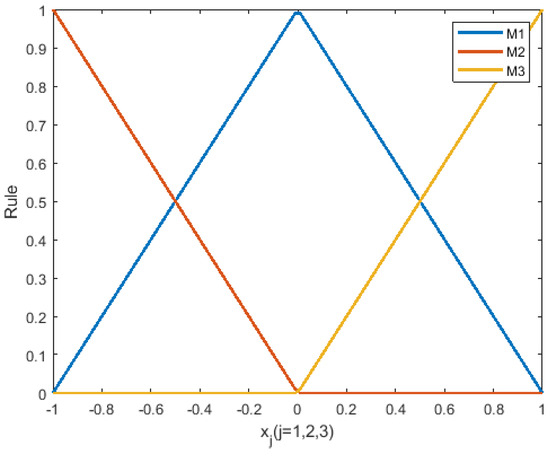
Figure 2. Membership functions of T-S fuzzy sets ${\mathcal{M}}_j^i\left(x_j\left(t\right)\right),j=1,2,3$.

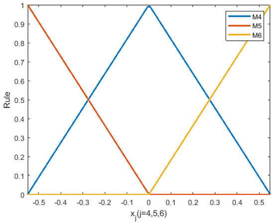
Figure 3. Membership functions of T-S fuzzy sets ${\mathcal{M}}_j^i\left(x_j\left(t\right)\right),j=4,5,6$.

Considering the previously mentioned three operating points, we can determine the values of the matrices $A_i$, $B_i$, and $C_i$ for $i=1,2,3$ in the presence of the external disturbance $d\left(t\right)$. These matrices are illustrated in Figure 4. In order to stabilize the flexible spacecraft system, matrix $\mathsf{\Theta }$ is provided as follows:

$$\begin{array}{c}\hfill \mathsf{\Theta }=\left[\begin{array}{ccc}-0.8& 0.3& 0.5\\ 0.5& -1& 0.5\\ 0.7& 0.6& -1.3\end{array}\right]\end{array}$$

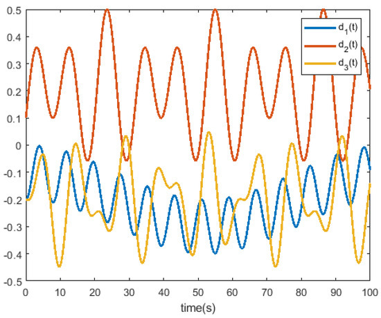
Figure 4. Simulation results of disturbance.

The sensor output matrices are given as follows: $L_1=0.8I$, $L_2=0.5I$, and $L_3=0.9I$. For $F_r$ and $G_r$, consider the following three cases.

Case I—a normal mode:

$$\begin{array}{c}\hfill F_1=I,G_1=0\end{array}$$

Case II—flawed operational state with partial loss of functionality:

$$\begin{array}{c}\hfill F_2=\left[\begin{array}{ccc}0.7& 0& 0\\ 0& 0.8& 0\\ 0& 0& 0.6\end{array}\right],G_2=0\end{array}$$

Case III—bias faulty mode:

$$\begin{array}{c}\hfill F_1=I,G_1=I\end{array}$$

The transition rate matrix for the nonhomogeneous Markov process is as follows:

$$\begin{array}{c}\hfill \mathsf{\Pi }\left(t\right)=co{s}^2\left(t\right){\mathsf{\Pi }}_1+si{n}^2\left(t\right){\mathsf{\Pi }}_2\end{array}$$

(52)

where

$$\begin{array}{c}\hfill {\mathsf{\Pi }}_1=\left[\begin{array}{ccc}-1.7& 0.9& 0.8\\ 1& -5& 4\\ 1.6& 1.1& -2.7\end{array}\right],{\mathsf{\Pi }}_2=\left[\begin{array}{ccc}-5& 2& 3\\ 0.1& -0.5& 0.4\\ 1& 1& -2\end{array}\right].\end{array}$$

(53)

Setting $\gamma =0.1$, ${\epsilon }_1=1$, ${\epsilon }_2=-0.1$, and $\mathsf{\Pi }\left(t\right)={\mathsf{\Pi }}_1$, and focusing solely on Case I, where $F_r=F_1$ and $G_r=G_1$, we utilize Theorem 2 to determine that the maximum allowable value for the upper bound of $c_2$ is $6.0114$. When considering all three cases under the same theorem, this upper bound is refined to $5.7741$. Notably, this finding surpasses the upper bound of $5.4$ previously established in [24]. From the above analysis, we draw three key conclusions:

C1: The comparison between $6.0114$ and the value reported in [24] ($5.4$) clearly demonstrates the superiority in the current study, signifying a notable enhancement in the system’s performance.

C2: Observing that the upper bound remains at $6.0114$ and $5.7741$ across different faults, it is evident that the system’s performance is optimized as fault tolerance is reduced. Thus, to achieve better system performance, one must tolerate smaller faults, and vice versa.

C3: It is important to highlight that the homogeneous case represents a special instance of the nonhomogeneous case as given in (52), with the latter being a more encompassing and general representation.

The three pivotal conclusions drawn highlight that the proposed method not only exhibits a more generalized framework but also outperforms existing models in terms of system performance.

Further, based on the condition specified in Equation (53), Theorem 2 provides the feedback gains as follows:

$$\begin{array}{ccc}\hfill K_{11}& =& \left[\begin{array}{cccccc}-152.2274& 29.9847& 12.2479& -45.5341& 5.7843& 2.0314\\ 25.4123& -164.5127& -4.8521& 4.2974& -48.2479& 0.1147\\ 14.5746& -7.2145& -72.1453& -5.4762& -0.7841& -45.4574\end{array}\right]\hfill \\ \hfill K_{21}& =& \left[\begin{array}{cccccc}-154.2149& 31.0146& 17.1142& -56.4046& 5.2194& 2.5448\\ 26.1417& -162.2747& -5.3147& 4.9413& -56.0141& 0.7412\\ 14.5172& -8.4547& -77.5314& -5.3118& -0.7468& 47.5741\end{array}\right]\hfill \\ \hfill K_{31}& =& \left[\begin{array}{cccccc}-151.1742& 30.1467& 18.1024& -59.1042& 4.9017& 2.9013\\ 26.1417& -162.2747& -5.3147& 4.9413& -56.0141& 0.9014\\ 12.1435& -8.4471& -76.1147& -6.2471& -0.7785& 45.9821\end{array}\right]\hfill \\ \hfill K_{12}& =& \left[\begin{array}{cccccc}180.5112& 90.5017& 41.1475& -54.4571& 5.8147& 2.2347\\ 207.2431& -165.2114& -13.8141& 5.0464& -62.0117& 2.0013\\ 0.1147& -25.1421& -102.1447& 3.2414& -1.2471& -30.9114\end{array}\right]\hfill \\ \hfill K_{22}& =& \left[\begin{array}{cccccc}175.1271& 88.5717& 40.7571& -55.0717& 4.9717& 3.4157\\ 202.4317& -162.0174& -18.1470& 54.1654& -60.1074& 3.1710\\ 1.0107& -21.2018& -12.4471& 4.0114& -2.0070& -19.1010\end{array}\right]\hfill \\ \hfill K_{23}& =& \left[\begin{array}{cccccc}177.4107& 85.0074& 47.5077& -50.7047& 7.1074& 4.1007\\ 240.0311& -120.1277& -14.5701& 51.6051& -61.0071& 1.7170\\ 1.1074& -20.0114& -14.4712& 41.0144& -0.0471& -11.0108\end{array}\right]\hfill \end{array}$$

When initializing the system with $x\left(0\right)=[2,-1.5,1,-2,1,-2]$, we can observe the state responses of the closed-loop fuzzy system in Figure 5 and Figure 6. These figures serve to highlight the effectiveness of the control design method, particularly when dealing with a nonhomogeneous Markovian process.

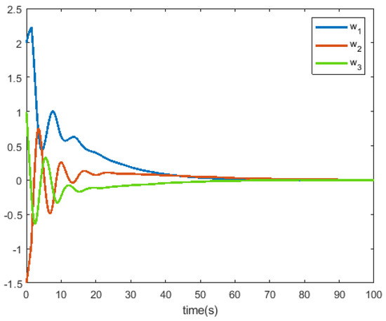
Figure 5. The state responses of w.

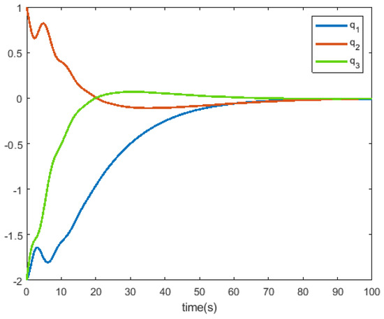
Figure 6. The state responses of q.

5. Conclusions

This paper has considered the formidable challenge of achieving finite-time fault-tolerant control in nonlinear flexible spacecraft systems that are susceptible to actuator faults. Our approach is grounded in the T-S fuzzy model methodology, where actuator failures are modeled as stochastic signals governed by a nonhomogeneous Markov process. To adeptly handle the complexities introduced by these components, we employ a representation of the nonhomogeneous Markov process as a polytope set. Our proposed solution involves the development of a robust nonhomogeneous Lyapunov stability framework, further enriched by the introduction of adaptable parameters. This innovative controller design methodology yields a stability criterion that guarantees $H_{\infty }$ performance in a mean-square sense. To empirically validate the efficacy of our approach, we present a numerical example featuring a nonlinear spacecraft system. This demonstration underscores the practical applicability and advantages of our proposed methodology. Future work will concentrate on extending this research to practical deployments and addressing unknown or unpredictable faults within the system.

References

- Xuan-Mung, N.; Golestani, M.; Nguyen, H.; Nguyen, N.; Fekih, A. Output feedback control for spacecraft attitude system with practical predefined-time stability based on anti-windup compensator. Mathematics 2023, 11, 2149. [Google Scholar] [CrossRef]
- Ma, J.; Wang, Z.; Wang, C. Hybrid attitude saturation and fault-tolerant control for rigid spacecraft without unwinding. Mathematics 2023, 11, 3431. [Google Scholar] [CrossRef]
- Li, A.; Liu, M.; Shi, Y. Adaptive sliding mode attitude tracking control for flexible spacecraft systems based on the Takagi-Sugeno fuzzy modelling method. Acta Astronaut. 2020, 175, 570–581. [Google Scholar] [CrossRef]
- Vimal Kumar, S.; Raja, R.; Marshal Anthoni, S.; Cao, J.; Tu, W. Robust finite-time non-fragile sampled-data control for T-S fuzzy flexible spacecraft model with stochastic actuator faults. Appl. Math. Comput. 2018, 321, 483–497. [Google Scholar] [CrossRef]
- Gu, Z.; Yue, D.; Park, J.; Xie, X. Memory-event-triggered fault detection of networked IT2 T-S fuzzy systems. IEEE Trans. Cybern. 2023, 53, 743–752. [Google Scholar] [CrossRef] [PubMed]
- Gu, Z.; Shi, P.; Yue, D.; Ding, Z. Decentralized adaptive event-triggered H∞ filtering for a class of networked nonlinear interconnected systems. IEEE Trans. Cybern. 2019, 49, 1570–1579. [Google Scholar] [CrossRef] [PubMed]
- Cheng, J.; Park, J.; Wang, H. Event-triggered H∞ control for T-S fuzzy nonlinear systems and its application to truck-trailer system. Appl. Math. Comput. 2016, 65, 62–71. [Google Scholar]
- Li, H.; Pan, Y.; Shi, P.; Shi, Y. Switched fuzzy output feedback control and its application to mass-spring-damping system. IEEE Trans. Fuzzy Syst. 2016, 24, 1259–1269. [Google Scholar] [CrossRef]
- Tian, Y.; Su, X.; Shen, C.; Ma, X. Exponentially extended dissipativity-based filtering of switched neural networks. Automatica 2024, 161, 111465. [Google Scholar] [CrossRef]
- Tian, Y.; Yang, Y.; Ma, X.; Su, X. Stability of discrete-time delayed systems via convex function-based summation inequality. Appl. Math. Lett. 2023, 143, 108764. [Google Scholar] [CrossRef]
- Liu, R.; Xing, L.; Deng, H.; Zhong, W. Finite-time adaptive fuzzy control for unmodeled dynamical systems with actuator faults. Mathematics 2023, 11, 2193. [Google Scholar] [CrossRef]
- Najafi, A.; Vu, M.T.; Mobayen, S.; Asad, J.; Fekih, A. Adaptive barrier fast terminal sliding mode actuator fault tolerant control approach for quadrotor UAVs. Mathematics 2022, 10, 3009. [Google Scholar] [CrossRef]
- Wang, B.; Shen, Y.; Zhang, Y. Active fault-tolerant control for a quadrotor helicopter against actuator faults and model uncertainties. Aerosp. Sci. Technol. 2020, 99, 105745. [Google Scholar] [CrossRef]
- Yang, H.; Jiang, Y.; Yin, S. Adaptive fuzzy fault-tolerant control for Markov jump systems with additive and multiplicative actuator faults. IEEE Trans. Fuzzy Syst. 2020, 29, 772–785. [Google Scholar] [CrossRef]
- Qiu, J.; Ding, S.; Gao, H.; Yin, S. Fuzzy-model-based reliable static output feedback H∞ control of nonlinear hyperbolic PDE systems. IEEE Trans. Fuzzy Syst. 2016, 24, 388–400. [Google Scholar] [CrossRef]
- Ahmed, T.S.; Muhammed, B.M.; Emmanuel, A.A.; Bashir, A.B. Optimal determination of hidden Markov model parameters for fuzzy time series forecasting. Sci. Afr. 2022, 16, e01174. [Google Scholar]
- Ding, K.; Lei, J.; Chan, F.; Hui, J.; Zhang, F.; Wang, Y. Hidden Markov model-based autonomous manufacturing task orchestration in smart shop floors. Robot. -Comput.-Integr. Manuf. 2020, 61, 101845. [Google Scholar] [CrossRef]
- Ahmed, T.S.; Patrick, J.N.; Hussein, U.S.; Izuagbe, S.M.; Emmanuel, K.A. Heuristic hidden Markov model for fuzzy time series forecasting. Int. J. Intell. Syst. Technol. Appl. 2021, 20, 146–166. [Google Scholar]
- Cheng, Y.; Li, S. Fuzzy time series forecasting with a probabilistic smoothing hidden Markov model. IEEE Trans. Fuzzy Syst. 2012, 20, 291–304. [Google Scholar] [CrossRef]
- Dharani, S.; Rakkaiyappan, R.; Cao, J. Robust stochastic sampled-data H∞ control for a class of mechanical systems with uncertainties. J. Dyn. Syst. Meas. Control. 2015, 137, 101008. [Google Scholar] [CrossRef]
- Hu, H.; Jiang, B.; Yang, H. Non-fragile H2 reliable control for switched linear systems with actuator faults. Signal Process. 2013, 93, 1804–1812. [Google Scholar] [CrossRef]
- Sun, G.; Xu, S.; Li, Z. Finite-time fuzzy sampled-data control for nonlinear flexible spacecraft with stochastic actuator failure. IEEE Trans. Ind. Electron. 2017, 64, 3851–3861. [Google Scholar] [CrossRef]
- Hu, S.; Yue, D.; Du, Z.; Liu, J. Reliable H∞ non-uniform sampling tracking control for continuous-time non-linear systems with stochastic actuator faults. IET Control. Theory Appl. 2012, 6, 120–129. [Google Scholar] [CrossRef]
- Wang, C.; Zhang, H.; Yang, S.; Bo, C.; Li, J. Fuzzy-model-based finite-time control of nonlinear spacecrafts over a distributed sensor network. J. Frankl. Inst. 2023, 360, 2729–2750. [Google Scholar] [CrossRef]
- Wang, D.; Wu, F.; Lian, J.; Li, S. Observer-Based asynchronous control for stochastic nonhomogeneous semi-Markov jump systems. IEEE Trans. Autom. Control. 2017, 62, 8. [Google Scholar] [CrossRef]
- Golmakani, M.; Hubbard, R.; Miglioretti, D. Nonhomogeneous Markov chain for estimating the cumulative risk of multiple false positive screening tests. Biometrics 2022, 78, 1244–1256. [Google Scholar] [CrossRef] [PubMed]
- Xu, C.; Wu, B.; Wang, D.; Zhang, Y. Decentralized event-triggered finite-time attitude consensus control of multiple spacecraft under directed graph. J. Frankl. Inst. 2021, 358, 9794–9817. [Google Scholar] [CrossRef]
- Gao, S.; Liu, X.; Jing, J.; Dimirovski, G. A novel finite-time prescribed performance control scheme for spacecraft attitude tracking. Aerosp. Sci. Technol. 2021, 118, 107044. [Google Scholar] [CrossRef]
- Amrr, S.; Nabi, M. Finite-time fault tolerant attitude tracking control of spacecraft using robust nonlinear disturbance observer with anti-unwinding approach. Adv. Space Res. 2020, 66, 1659–1671. [Google Scholar] [CrossRef]
- Lee, D. Fault-tolerant finite-time controller for attitude tracking of rigid spacecraft using intermediate quaternion. IEEE Trans. Aerosp. Electron. Syst. 2020, 57, 540–553. [Google Scholar] [CrossRef]
- Zheng, C.; Cao, J.; Hu, M.; Fan, X. Finite-time stabilisation for discrete-time T-S fuzzy model system with channel fading and two types of parametric uncertainty. Int. J. Syst. Sci. 2017, 48, 34–42. [Google Scholar] [CrossRef]
- Gu, C.; Chen, J.; Kharitonov, V. Stability of Time-Delay Systems; Springer: Boston, MA, USA, 2003. [Google Scholar]
- Feng, Z.; Lam, J.; Yang, G. Optimal partitioning method for stability analysis of continuous/discrete delay systems. Int. J. Robust Nonlinear Control. 2015, 25, 559–574. [Google Scholar] [CrossRef]
- Zhang, H.; Liu, Z. Stability analysis for linear delayed systems via an optimally dividing delay interval approach. Automatica 2011, 47, 2126–2129. [Google Scholar] [CrossRef]
- Jiang, B.; Karimi, H.; Yang, S.; Gao, C.; Kao, Y. Observer-based adaptive sliding mode control for nonlinear stochastic Markov jump systems via T-CS fuzzy modeling: Applications to robot arm mdel. IEEE Trans. Ind. Electron. 2020, 68, 466–477. [Google Scholar] [CrossRef]
- Nguyen, A.; Sentouh, C.; Zhang, H.; Popieul, J. Fuzzy static output feedback control for path following of autonomous vehicles with transient performance improvements. IEEE Trans. Intell. Transp. Syst. 2019, 21, 3069–3079. [Google Scholar] [CrossRef]
- Liu, H.; Pan, Y.; Cao, J.; Wang, H.; Zhou, Y. Adaptive neural network backstepping control of fractional-order nonlinear systems with actuator faults. IEEE Trans. Neural Netw. Learn. Syst. 2020, 31, 5166–5177. [Google Scholar] [CrossRef] [PubMed]
- Zhang, H.; Liang, Y.; Su, H.; Liu, C. Event-driven guaranteed cost control design for nonlinear systems with actuator faults via reinforcement learning algorithm. IEEE Trans. Syst. Man Cybern. Syst. 2020, 50, 4135–4150. [Google Scholar] [CrossRef]
- Liu, Z.; Han, Z.; Zhao, Z.; He, W. Modeling and adaptive control for a spatial flexible spacecraft with unknown actuator failures. Sci. China Inf. Sci. 2021, 64, 1–16. [Google Scholar] [CrossRef]
- Liu, Q.; Liu, M.; Shi, Y.; Yu, J. Event-triggered adaptive attitude control for flexible spacecraft with actuator nonlinearity. Aerosp. Sci. Technol. 2020, 6106, 106111. [Google Scholar] [CrossRef]
Disclaimer/Publisher’s Note: The statements, opinions and data contained in all publications are solely those of the individual author(s) and contributor(s) and not of MDPI and/or the editor(s). MDPI and/or the editor(s) disclaim responsibility for any injury to people or property resulting from any ideas, methods, instructions or products referred to in the content. |
© 2024 by the authors. Licensee MDPI, Basel, Switzerland. This article is an open access article distributed under the terms and conditions of the Creative Commons Attribution (CC BY) license (https://creativecommons.org/licenses/by/4.0/).