Abstract
In this work, we present both analytical and numerical solutions to a seven-parameter confluent Heun-type differential equation. This second-order linear differential equation features three singularities: two regular singularities and one irregular singularity at infinity. First, employing the tridiagonal representation method (TRA), we derive an analytical solution expressed in terms of Jacobi polynomials. The expansion coefficients of the series are determined as solutions to a three-term recurrence relation, which is satisfied by a modified form of continuous Hahn orthogonal polynomials. Second, we develop a numerical scheme based on the basis functions used in the TRA procedure, enabling the numerical solution of the seven-parameter confluent Heun-type differential equation. Through numerical experiments, we demonstrate the robustness of this approach near singularities and establish its superiority over the finite difference method.
Keywords:
continuous Hahn polynomials; confluent Heun’s differential equation; tridiagonal representation; recurrence relation; orthogonal polynomials; finite difference method; stability MSC:
34A05; 34A25; 33C45; 34B30
1. Introduction
Differential equations are a fundamental tool in describing physical phenomena, with theoretical physicists investing considerable effort in developing tools for finding their solutions. The nature and types of singularities in these equations are crucial in understanding and controlling the richness of physical phenomena. In science and engineering, differential equations are widely used to model systems, creating an extensive list of solutions. The classification of these equations includes ordinary [1], partial [2], fractional [3], and differential–algebraic [4], and they are categorized based on linearity, order, and degree. In this work, a second-order linear differential equation with singularities is solved using a special approach.
The tridiagonal representation approach (TRA) is a method widely used in physics to solve quantum mechanical problems. It is inspired by the J-matrix method discussed in [5,6], which started using the TRA technique as a mathematical tool. Although the initial literature related to TRA dates back to [7], a modern operator-theoretic TRA setup is established in [8] and references therein. The TRA transforms the differential equation into a three-term recurrence relation, which is subsequently solved using orthogonal polynomials, yielding expansion coefficients [9].
The study of the five-parameter Laguerre-type differential equation
has been recently carried out in [10]. Under the constraints arising either physically or due to the tridiagonal requirement, the series solution of (1) can be expressed in terms of Laguerre polynomials, where the expansion coefficients correspond to various orthogonal polynomials. These include the two-parameter Meixner–Pollaczek polynomial [10] [Section 2.1.1], the discrete Meixner polynomial [10] [Section 2.1.2], the discrete Krawtchouk polynomial [10] [Section 2.1.3], the three-parameter dual Hahn polynomial [10] [Section 2.2.1], and the discrete dual Hahn polynomial [10] [Section 2.2.2]. In the same paper, the author also analyzed a six-parameter Jacobi type differential equation
The solution is expressed as a square summable series having coefficients either as the four-parameter Wilson polynomial ([10] [Section 3.2.1]) or the discrete Racah polynomial ([10] [Section 3.2.2]) and basis elements formed using Jacobi polynomials for specific parameter relationships between the basis element and the differential Equation (2). Two new families of orthogonal polynomials are encountered while solving (2) under some specific tridiagonal conditions ([10] [Sections 3.1.1 and 3.1.2]).
Another six-parameter differential equation of Bessel type
is considered in [11]. It is observed that a series solution in terms of the Bessel basis is possible when coefficients happen to be discrete Hahn polynomials ([11] [Section 3.1]). In the other cases, a singular Laguerre basis is used to express the solution of (3) as a series having coefficients either from the Meixner–Pollaczek polynomial and its modified version ([11] [Sections 6.1 and 6.3]) or the dual Hahn polynomial ([11] [Section 6.2]).
The nine-parameter Heun type differential equation
where are real parameters and , is treated using TRA. For and with , the original Heun equation is obtained [12]. As a consequence of the tridiagonal requirement, four sets of constraints involving basis parameters and parameters of (4) arise. Under these constraints, three solutions to the differential equation (4) are demonstrated as series representations in terms of Jacobi polynomials having coefficients as Wilson polynomials [13] [Section II], modified Wilson polynomials [13] [Section III], and a new four-parameter orthogonal polynomial [13] [Section IV]. These three solutions are called the restricted solution, the generalized solution, and the special solution, respectively.
The differential Equation (4) has four regular singular points: . Four confluent differential equations are formed through the confluence of these regular singularities, each having an irregular singular point either at zero or infinity. These are confluent, double confluent, biconfluent, and triconfluent Heun’s equation, often abbreviated as CHE, DHE, BHE, and THE, respectively. Various confluent forms of Heun’s differential equation, their solution, and their properties have attracted the interest of experts in the field for a long time, e.g., the study of derivatives of CHE, DHE, BHE, and THE is carried out in [14]. Solutions to these equations using operator theoretic factorization can be found in [15]. For a compendium on Heun’s differential equation and its various deformations, refer to [16].
It is important to note that (2) is commonly known as a hypergeometric-type differential equation, with regular singular points at 1, , and . Through the confluence process, (2) transforms into (1), which has a regular singularity at 0 and an irregular singularity at ; and, hence, (1) is also known as a confluent hypergeometric-type differential equation. Motivated by the studies mentioned above, the TRA treatment is extended to a seven-parameter confluent Heun-type differential equation solution
and are real parameters. The original confluent Heun equation corresponds to , , , , , and . Furthermore, we have observed a notable absence of numerical solutions for (5) in the existing literature. Given the equation’s profound real-world applications, we believe that developing a numerical solution could unlock a broader range of applications across various scientific fields. This research paper aims to bridge this gap in the study of confluent-type Heun equations by proposing a numerical scheme that closely aligns with traditional spectral methods in numerical analysis, which are often based on orthogonal polynomials. Two specific examples of equations that take the form of the confluent Heun differential equation and describe real-world physical phenomena are as follows:
1.1. Teukolsky Equation for Perturbations of a Kerr Black Hole
The Teukolsky equation describes perturbations (scalar, electromagnetic, or gravitational) of a Kerr black hole [17]. For a scalar field perturbation, the radial part of the equation takes the form
where and are the radii of the event horizon and Cauchy horizon of the Kerr black hole and A, B, C, D are constants depending on the black hole parameters and the perturbation mode. The Teukolsky equation is fundamental in the study of black hole physics. It describes how scalar, electromagnetic, or gravitational waves propagate in the curved spacetime around a rotating (Kerr) black hole. The solutions to this equation provide information about quasinormal modes (oscillations of black holes) and wave-scattering phenomena, which are crucial for understanding black hole dynamics and gravitational wave signals detected by observatories like LIGO and Virgo. Further studies exploring the relationship between the confluent Heun equation and black hole perturbation theory can be found in [18] and the references therein.
1.2. Schrödinger Equation for the Hydrogen Atom in an External Electric Field (Stark Effect)
The Schrödinger equation for a hydrogen atom in a uniform external electric field [19] (Stark effect) can be reduced to a confluent Heun equation. The radial part of the wavefunction satisfies
where Z is the atomic number, E is the energy eigenvalue, and F is the strength of the external electric field. The Stark effect describes the shifting and splitting of spectral lines of atoms and molecules due to the presence of an external electric field. The confluent Heun equation arises when solving the Schrödinger equation for the hydrogen atom in such a field, providing insights into the energy levels and wavefunctions of the system. We encourage interested readers to refer to [20] and the references therein for a more detailed exploration of the interplay between the Schrödinger equation and the confluent Heun equation.
The rest of the paper is summarized as follows: Auxiliary material required in further sections of the paper is detailed in Section 2. In Section 3, the solution of (5) is written as an infinite series of square integrable functions having coefficients , i.e.,
A modified continuous Hahn orthogonal polynomial is discovered to satisfy a three-term recurrence relation, which yields the coefficients . A description of two numerical schemes for solving (5) is provided in Section 4. Numerical results are presented for various parameter values of the differential Equation (5), and a stability comparison of both methods is conducted. To the best of the authors’ knowledge, such a numerical analysis of confluent-type differential equations has not been explored in the existing literature. Furthermore, in Section 5, a comparison is made between the theoretical results available in the literature and those obtained in this work for (5). In particular, a noteworthy comparison with the findings of [21] is highlighted, and potential directions for future research are discussed.
2. Preliminaries
First of all in this technique, the basis functions that can solve the differential equation are selected. Hence, the following basis elements can be proposed based on the singularity structure of (5):
Here, represents the normalization constant, and denotes the Jacobi polynomial, which is defined as follows:
where , and . The function is the gamma function defined as follows:
and the function is the generalized hypergeometric function defined as follows:
where is the Pochhammer symbol, defined as
Further, in the TRA technique, the parameters of the basis are related to the parameters of (5) either by square integrability of or by the TRA requirement on coefficients . Expressions (8)–(12) serve as auxiliary material that we will be using frequently in the due course of this paper. The first- and second-order derivatives of basis elements can be obtained as follows:
The differential equation
and differential property
of Jacobi polynomials together with the recurrence relation
makes it possible for the operator acting on basis elements to produce terms that are proportional to , and up to multiplication by a constant. The parameters of the basis will be related to the parameters of (5) either by square integrability of or by the TRA requirement on coefficients , and we have
where . Note that (5) can also be represented as (). Substituting (6) in (5), we have
which implies that the coefficients should satisfy
where and is some function of the parameters . The recurrence coefficients , , , and depend on j and the parameters , but are independent of . Further, the condition guarantees the existence of a positive definite moment functional with respect to which there exists a sequence of orthogonal polynomials satisfying (14) and defined as . This implies and , if we assume . With and as initial values, recursion (14) can be used to generate polynomials of the desired degree, and it can be easily established that is a polynomial of degree j. Thus, the solution of (14) becomes equivalent to the solution of (5), which enables us to study the properties of associated physical systems (structural and dynamical) from the properties (e.g., weight function, generating function, asymptotics, orthogonality relation, zeros, and differential or difference relations [22]) of these polynomials.
3. The TRA Solution
Our attempt is to convert the L.H.S. of differential Equation (5) into an equation of the form (13) where only linear or contant terms are allowed to multiply with , , and .
Theorem 1.
If the parameters, A and B, of the differential equation are below critical values, i.e., 4 and 4, then (5) reduces to a three-term recurrence equation involving , , and , written as
where
Proof.
The action of operator on the basis elements (7) with use of (8) and (9) yields
Expanding the power and multiplying the requisite brackets, we have
Collecting similar terms, we obtain
Taking the factor inside the brackets and using (10), we have
Use of some simple algebraic identities gives
Again collecting similar terms together, we have
Using (11), we obtain
The tridiagonal requirement suggests that the coefficient of the quadratic term and of the fractional terms and must vanish. As discussed earlier, these restrictions prescribe the following values to basis parameters . That is,
Putting these value in (16), we obtain
where the signs ± and ∓ corresponds to the two choices of , i.e., and , respectively, which also governs the value of in the basis (7). Using (12), we have
Simplifyng the coefficients of and , respectively, we obtain
Choosing
and rewriting (17) in terms of , we have
which implies
and the proof is complete. □
Using the fact that (5) can be represented as , (15) is reduced to a relation of the form (14) in the next theorem.
Theorem 2.
The solutions of the recurrence obtained for expansion coefficients
are the modified continuous Hahn polynomials and the solution of the seven-parameter confluent Heun-type differential equation becomes
where is the normalization factor, and the modified polynomial parameters are given as
Proof.
In the view of
and (since ), (18) gives the recurrence for expansion coefficients (19). Note that the recurrence relation (19) is of the form
where
Evidently, the recursion (21) happens to be the modified version of the following well-known recurrence
and polynomial is the continuous Hahn polynomial [23] defined as
Hence, the polynomials that are sought to act as the expansion coefficients in (6) are the modified version of the continuous Hahn polynomial having as a deformation factor and that completes the proof. □
Remark 1.
In (20), is the normalization factor proportional to the square root of the weight function of modified continuous Hahn polynomials that are yet to be derived.
Given the fact that (5) has singularities at points and , the problem of convergence of the series solution (20) is worth considering. The next theorem deals with convergence analysis of the series .
Theorem 3.
If for , then the series converges.
Proof.
It is known that any hypergeometric function of the form , where , is convergent for [24]. This implies that the series is convergent for . In other words, the function is a finite sum because the first parameter is a negative integer. This means it is a polynomial in x of degree j. For large j, the growth of is controlled by the highest power of x, which is . Note that decays polynomially for as . Further, the function is also convergent for or . In other words, the function being a polynomial of degree j, its growth is controlled by the highest power of , which is . Therefore, each term of the sequence behaves like
For large j, the term decays exponentially for . It remains to analyse the behaviour of for large j.
Using Stirling’s approximation for the gamma function [25]
we approximate the denominator for large j
Thus, the denominator becomes
The numerator is
For large j, this behaves like . Combining the numerator and denominator, we obtain
Simplifying further, we have
For large j, approximate and :
Notice that . Thus,
For large j, the dominant term is , which decays super-exponentially (faster than any exponential or polynomial decay). Therefore, the sequence decays super-exponentially as . Therefore, the sequence is convergent for or, more precisely, for any , . Summarizing, we have a series that is convergent for (subset of ) and a convergent sequence on the same domain. Hence, the theorem is proved using Abel’s test for series. □
4. Numerical Experiments
Spectral methods in numerical analysis for solving differential equations typically involve selecting basis functions in such a way that any singularity present in the equation is either removed or significantly weakened. The TRA approach presented above not only facilitates obtaining an analytical solution to (5) but also aids in formulating a numerical scheme based on the basis elements . For brevity, we refer to this method as the “spectral method using ()” henceforth. The various steps involved in computing the numerical solution of (5) are outlined below.
- Truncate the domain to avoid singularities at and . Let the truncated domain be for very small and positive.
- Expand the solution in terms ofwhere are expansion coefficients.
- Discretize the differential equation to obtain a system of linear equations
- Modify the system to enforce the boundary conditions.
- Solve the resulting system of linear equations for the coefficients .
- Reconstruct and plot the solution using the computed coefficients.
- Vary to check the stability and accuracy of the method.
A comparison of this numerical scheme with a traditionally existing numerical scheme called the finite difference method (FDM) [26] has been carried out. Typical steps in FDM are as follows:
- We solve the equation on the truncated domain where is a small positive number.
- The finite difference method approximates the derivatives as follows:where h is the step size.
- The discretized equation at grid point isThis can be rewritten aswhere
- The matrix is set up using the coefficients .
- The boundary conditions are enforced by setting the corresponding rows of the matrix and right-hand side.
- The system of equations is solved using a numerical linear algebra solver.
- Solves the problem for different values of and plot the solutions to check the stability and accuracy of the method.
From (6) and (7), it is evident that and need to be imposed as boundary conditions for numerical simulation. Note that the system of equations obtained on discretizing (5) will be a homogeneous system. Now, if the system has a unique solution, it has to be the zero solution. To avoid such a situation and to obtain a unique numerical solution, boundary conditions are adjusted to make the system non-homogeneous. Further, we have considered the truncated domain as per Theorem 3 for obtaining the solutions. The numerical solutions of (5) using FDM and for fixed values of parameters are plotted from Figure 1, Figure 2, Figure 3 and Figure 4. Alongside, by varying , the stability of the system is analysed. The selected parameter values satisfy critical conditions outlined in Theorem 1.
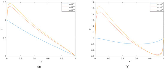
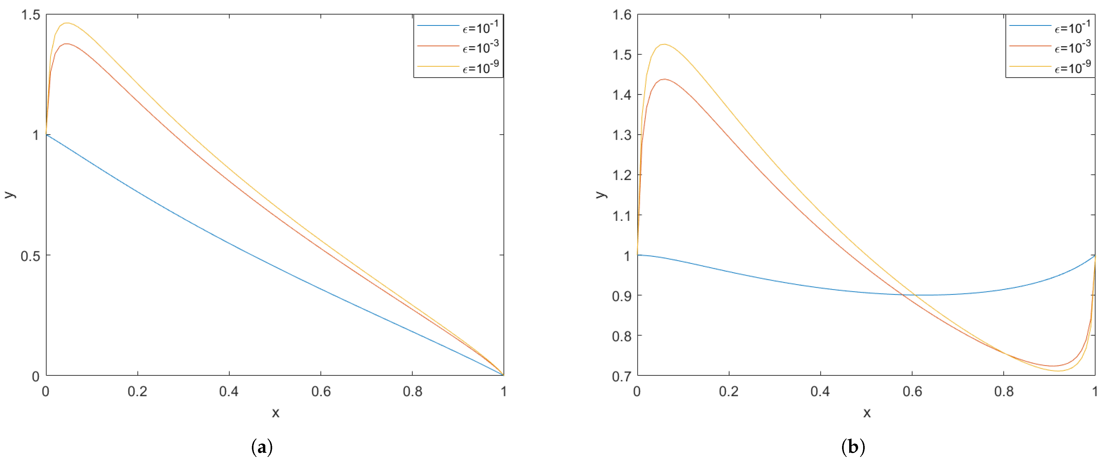
Figure 1.
(a) Plot of using and having boundary condition and . (b) Plot of using and having boundary condition and . Both plots assume the parameter values as .
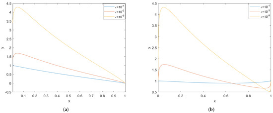
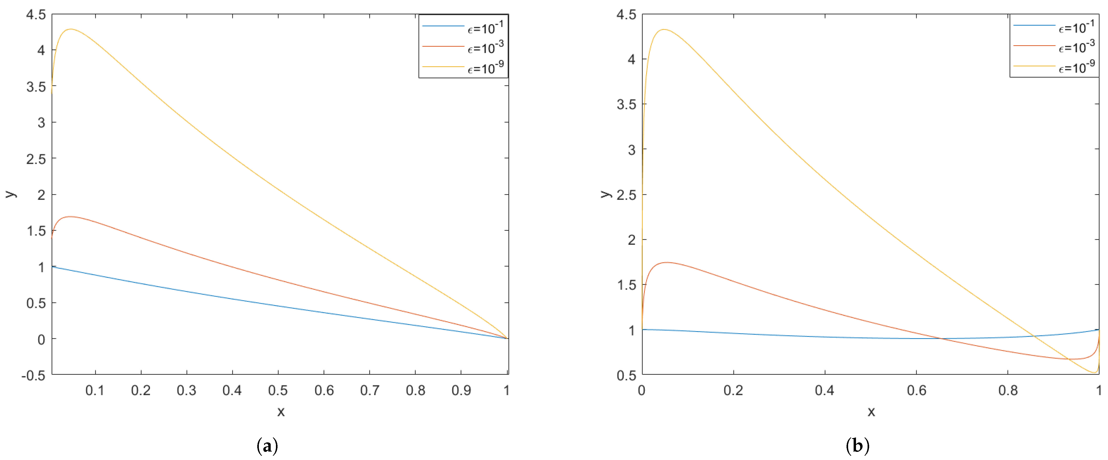
Figure 2.
(a) Plot of using FDM and having boundary condition and . (b) Plot of using FDM and having boundary condition and . Both plots assume the parameter values as .
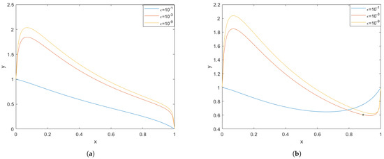
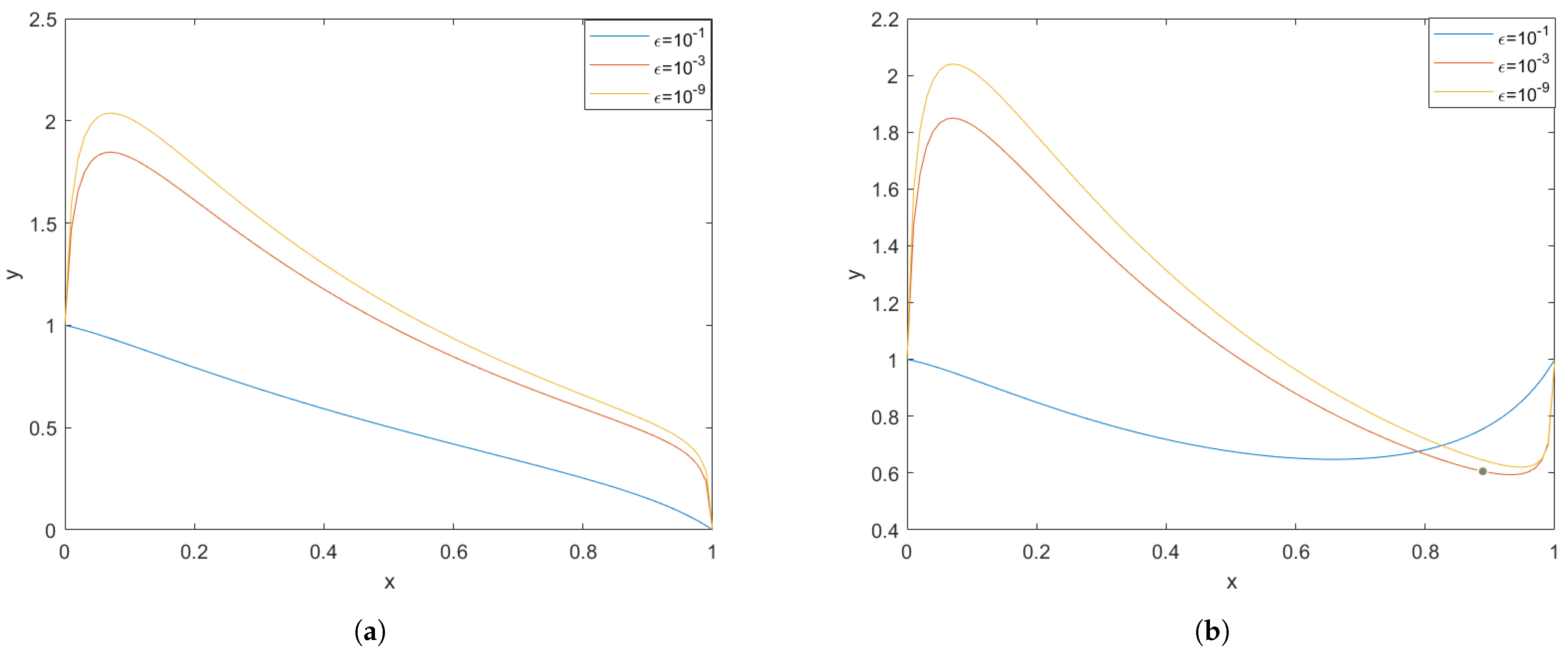
Figure 3.
(a) Plot of using and having boundary condition and . (b) Plot of using and having boundary condition and . Both plots assume the parameter values as .
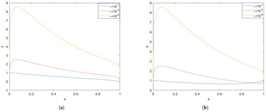
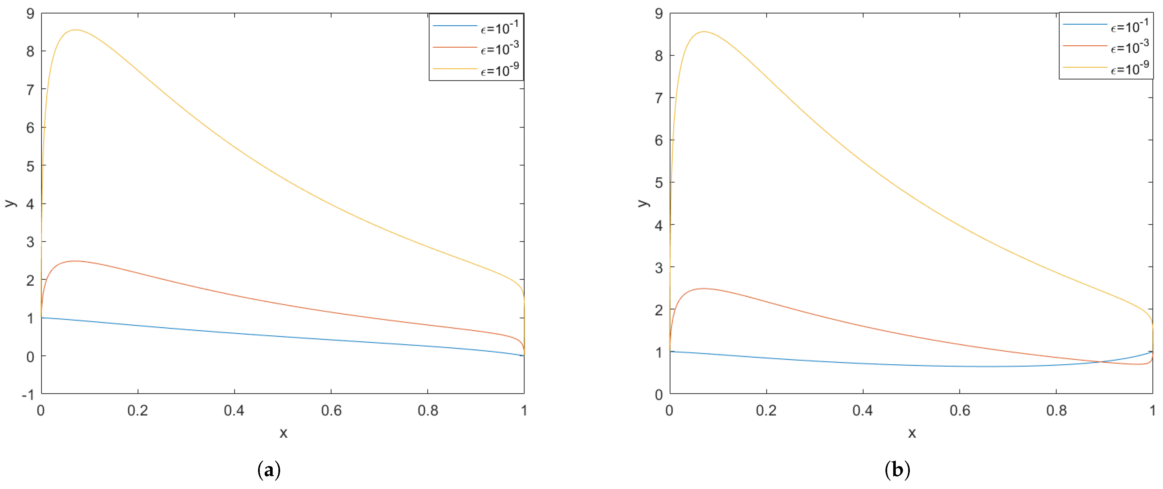
Figure 4.
(a) Plot of using FDM and having boundary condition and . (b) Plot of using FDM and having boundary condition and . Both plots assume the parameter values as .
4.1. Computational Setup
The numerical computations were performed on a system equipped with an Intel Core i5 processor and 8 GB of RAM. The implementation was carried out using MATLAB R2023b. The grid was constructed with N = 100 points, ensuring a sufficiently fine resolution while maintaining computational efficiency. The resulting tridiagonal system was solved using direct matrix inversion in MATLAB. The condition number of the system matrix was computed to assess the numerical stability. Visualizations of the solutions were generated using the built-in plotting functions in MATLAB. The computations were carried out on a standard workstation without requiring high-performance computing (HPC) resources.
4.2. Significance of Figure 1 and Figure 2
It can be observed that Figure 1a and Figure 2a correspond to the same parameter values and identical boundary conditions, and . From Figure 2a, it is evident that, as decreases, or as we approach the singularity at , the solution becomes increasingly unstable. Furthermore, this instability grows at a faster rate in the finite difference method (FDM) compared to for the same , as seen in the yellow curves in Figure 1a and Figure 2a. Similarly, Figure 1b and Figure 2b also share the same parameter values and boundary conditions, and . Here too, a decrease in leads to instability near , and comparing the yellow curves reveals that this instability progresses more rapidly in Figure 2b than in Figure 1b.
4.3. Significance of Figure 3 and Figure 4
Figure 3a and Figure 4a depict solutions obtained using identical parameter values and boundary conditions and . A closer examination of Figure 3a reveals that, as decreases or as we approach the singularity at , the solution exhibits increasing instability. Notably, this instability develops more rapidly in the finite difference method (FDM) compared to , as evidenced by the yellow and red curves in Figure 3a and Figure 4a. Likewise, Figure 3b and Figure 4b share the same set of parameters and boundary conditions, and . In this case, a similar pattern emerges: decreasing leads to solution instability near . A comparison of the yellow and red curves further indicates that the rate of instability growth is higher in Figure 4b than in Figure 3b.
It can be concluded that the results obtained from the spectral method using provide better solutions than the FDM method to the differential Equation (5) in terms of stability.
5. Conclusions and Future Scope
For the confluent-type Heun equation of the form (5), various solution approaches already exist in the literature. These include a polynomial solution [27], a series solution expressed in terms of the generalized hypergeometric function [28], and a series solution formulated using the incomplete beta function [29]. However, in this study, we introduce a novel solution to (5) based on orthogonal polynomials, offering a fresh perspective on solving this class of equations. The necessity of series solutions can be accessed from the fact that they are well-suited for handling singularities, as they allow us to express the solution as a power series around these points. Moreover, the confluent Heun equation generally does not have a simple closed-form solution. Series solutions are one of the few methods that can provide explicit representations of the solution. The advantage of having series solutions is that they can be adapted to different forms (e.g., power series, asymptotic series) depending on the region of interest (e.g., near a singularity or at infinity). Further, the process of obtaining series solution for (5) motivated us to seek numerical solutions using efficient algorithms, making them practical for computational purposes. Series solutions can be truncated to a finite number of terms for numerical computation, providing an efficient way to approximate the solution. The necessities and advantages of obtaining series solutions have been widely emphasized in several existing studies in this direction, such as [27,28,29], among others.
In the investigation detailed in [21], a 10-parameter second-order linear differential equation is explored, revealing modified continuous Hahn polynomials as the expansion coefficients. Notably, in this study, the recursion coefficients and are both influenced by the deformation factor , a distinction from [21] [Equation (28)]. Additionally, the validity of the TRA is established when the differential equation parameter [21] [Equation (5)]. Since, the CHE (5) is formed by the confluence of two singularities, it should not be confused with the case in [21] since is a singularity separately handled in that paper. This fact underscores the independence of the proof presented in this study.
It would be interesting to extend TRA treatment for finding series solutions of the following biconfluent (22) and triconfluent (23) Heun equations in terms of orthogona polynomials.
Author Contributions
Conceptualization, V.K. and S.R.M.; methodology, V.K. and S.R.M.; validation, V.K. and S.R.M.; formal analysis, V.K. and S.R.M.; writing—original draft preparation, V.K. and S.R.M.; writing—review and editing, V.K. and S.R.M. All authors have read and agreed to the published version of the manuscript.
Funding
This work was supported by the Deanship of Scientific Research, Vice Presidency for Graduate Studies and Scientific Research, King Faisal University, Saudi Arabia [Grant No. KFU251261].
Data Availability Statement
The original contributions presented in this study are included in the article. Further inquiries can be directed to the corresponding author.
Acknowledgments
We thank the reviewers for their constructive criticism that helped in the improvement of the manuscript.
Conflicts of Interest
The authors declare no conflicts of interest.
References
- Aloui, B.; Chammam, W. Classical orthogonal polynomials via a second-order linear differential operators. Indian J. Pure Appl. Math. 2020, 51, 689–703. [Google Scholar] [CrossRef]
- Ali, M.; Giri, A.K. A note on the discrete coagulation equations with collisional breakage. Acta Appl. Math. 2024, 189, 5. [Google Scholar] [CrossRef]
- Abdalla, M.; Akel, M. Contribution of using Hadamard fractional integral operator via Mellin integral transform for solving certain fractional kinetic matrix equations. Fractal Fract. 2022, 6, 305. [Google Scholar] [CrossRef]
- Shukla, V.; Swaminathan, A. Stability of the Toda system related to a perturbed RI type recurrence relation. arXiv 2024, arXiv:2406.09743. [Google Scholar] [CrossRef]
- Ismail, M.E.H.; Koelink, E. The J-matrix method. Adv. Appl. Math. 2011, 46, 379–395. [Google Scholar] [CrossRef]
- Ismail, M.E.H.; Koelink, E. Spectral properties of operators using tridiagonalization. Anal. Appl. 2012, 10, 327–343. [Google Scholar] [CrossRef]
- Heller, E.J.; Yamani, H.A. J-matrix method: Application to S-wave electron–hydrogen scattering. Phys. Rev. A 1974, 9, 1209–1214. [Google Scholar] [CrossRef]
- Genest, V.X.; Ismail, M.E.H.; Vinet, L.; Zhedanov, A. Tridiagonalization of the hypergeometric operator and the Racah-Wilson algebras. Proc. Am. Math. Soc. 2016, 144, 4441–4454. [Google Scholar] [CrossRef]
- Alhaidari, A.D. Orthogonal polynomials derived from the tridiagonal representation approach. J. Math. Phys. 2018, 59, 013503. [Google Scholar] [CrossRef]
- Alhaidari, A.D. Series solutions of Laguerre- and Jacobi-type differential equations in terms of orthogonal polynomials and physical applications. J. Math. Phys. 2018, 59, 063508. [Google Scholar] [CrossRef]
- Alhaidari, A.D.; Bahlouli, H. Solutions of a Bessel-type differential equation using the tridiagonal representation approach. Rep. Math. Phys. 2021, 87, 313–327. [Google Scholar] [CrossRef]
- Magnus, A.P.; Ndayiragije, F.; Ronveaux, A. About families of orthogonal polynomials satisfying Heun’s differential equation. J. Approx. Theory 2021, 263, 105522. [Google Scholar] [CrossRef]
- Alhaidari, A.D. Series solutions of Heun-type equation in terms of orthogonal polynomials. J. Math. Phys. 2018, 59, 113507. [Google Scholar] [CrossRef]
- Hounkonnou, M.N.; Ronveaux, A. About derivatives of Heun’s functions from polynomial transformations of hypergeometric equations. Appl. Math. Comput. 2009, 209, 421–424. [Google Scholar] [CrossRef]
- Hounkonnou, M.N.; Ronveaux, A.; Sodoga, K. Factorization of some confluent Heun’s differential equations. Appl. Math. Comput. 2007, 189, 816–820. [Google Scholar] [CrossRef]
- Ronveaux, A. Heun’s Differential Equations; Oxford University Press: Oxford, UK, 1995. [Google Scholar]
- Hussain, A.; Zimmerman, A. Approach to computing spectral shifts for black holes beyond Kerr. Phys. Rev. D 2022, 106, 104018. [Google Scholar] [CrossRef]
- Minucci, M.; Panosso Macedo, R. The confluent Heun functions in black hole perturbation theory: A spacetime interpretation. Gen. Relativ. Gravit. 2025, 57, 33. [Google Scholar] [CrossRef]
- Osherov, V.I.; Ushakov, V.G. Analytical solutions of the Schrödinger equation for a hydrogen atom in a uniform electric field. Phys. Rev. A 2017, 95, 023419. [Google Scholar] [CrossRef]
- Figueiredo, B.D.B. Schrödinger equation as a confluent Heun equation. Phys. Scr. 2025, 99, 055211. [Google Scholar] [CrossRef]
- Alhaidari, A.D. Series solution of a ten-parameter second-order differential equation with three regular singularities and one irregular singularity. Theor. Math. Phys. 2020, 202, 17–29. [Google Scholar] [CrossRef]
- Ismail, M.E.H. Classical and Quantum Orthogonal Polynomials in One Variable; Encyclopedia of Mathematics and Its Applications, 98; Cambridge University Press: Cambridge, UK, 2005. [Google Scholar]
- Koekoek, R.; Lesky, P.A.; Swarttouw, R.F. Hypergeometric Orthogonal Polynomials and Their q-Analogues; Springer: Berlin/Heidelberg, Germany, 2010. [Google Scholar]
- Rainville, E.D. Special Functions; The Macmillan Company: New York, NY, USA, 1960. [Google Scholar]
- Andrews, G.E.; Askey, R.; Roy, R. Special Functions; Cambridge University Press: Cambridge, UK, 1999; Volume 71, pp. xvi+–664. [Google Scholar]
- Thomas, J.W. Numerical Partial Differential Equations: Finite Difference Methods; Springer Science & Business Media: Berlin/Heidelberg, Germany, 2013; Volume 22. [Google Scholar]
- Lévai, G. Potentials from the polynomial solutions of the confluent Heun equation. Symmetry 2023, 15, 461. [Google Scholar] [CrossRef]
- Ishkhanyan, T.A.; Ishkhanyan, A.M.; Cesarano, C. Solutions of a Confluent Modification of the General Heun Equation in Terms of Generalized Hypergeometric Functions. Lobachevskii J. Math. 2023, 44, 5258–5265. [Google Scholar] [CrossRef]
- Ishkhanyan, A.M. Series solutions of confluent Heun equations in terms of incomplete gamma-functions. J. Appl. Anal. Comput. 2019, 9, 118–139. [Google Scholar] [CrossRef]
Disclaimer/Publisher’s Note: The statements, opinions and data contained in all publications are solely those of the individual author(s) and contributor(s) and not of MDPI and/or the editor(s). MDPI and/or the editor(s) disclaim responsibility for any injury to people or property resulting from any ideas, methods, instructions or products referred to in the content. |
© 2025 by the authors. Licensee MDPI, Basel, Switzerland. This article is an open access article distributed under the terms and conditions of the Creative Commons Attribution (CC BY) license (https://creativecommons.org/licenses/by/4.0/).