A New Family of Buckled Rings on the Unit Sphere

Abstract

Buckled rings, also known as pressurized elastic circles, can be described as critical points for a variational problem, namely the integral of a quadratic polynomial in the geodesic curvature of a curve. Thus, they are a generalization of elastic curves, and they are solitary wave solutions to a flow in a (three-dimensional) filament hierarchy. An example of such a curve is the Kiepert Trefoil, which has three leaves meeting at a central singular point. Such a variational problem can be considered for curves in other surfaces. In particular, researchers have found many examples of such curves in a unit sphere. In this article, we consider a new family of such curves, having a discrete dihedral symmetry about a central singular point. That is, these are spherical analogues of the Kiepert curve. We determine such curves explicitly using the notion of a Killing field, which is a vector field along a curve that is the restriction of an isometry of the sphere. The curvature k of each such curve is given explicitly by an elliptic function. If the curve is centered at the south pole of the sphere and has minimum value $\rho$, then $k-\rho$ is linear in the height above the pole.

1. Introduction

The classical elastica or elastic curve is a curve that is critical for the total squared curvature ${\int }_{\gamma }(k^2+\lambda )ds$, where k is the (geodesic) curvature of the curve $\gamma$ in the plane ${\mathbb{R}}^2$ or space ${\mathbb{R}}^3$, and $\lambda$ is a Lagrange multiplier acting to constrain the length of the curve. This is essentially the model of an elastic rod in equilibrium proposed by Daniel Bernoulli in 1743 in a letter to Euler. Using his newly developed Calculus of Variations, Euler was able to find a good qualitative description of all planar elastic curves.

In 1884, Maurice Lévy [1] developed a model of an elastic circle under uniform normal pressure, which was relevant to the consideration of the stability of boiler tubes and flues and of the buckling of steel plates of a ship. This was later studied by by Halphen [2] and Greenhill [3]. Imagine a cylindrical pipe with circular cross-section made of some flexible but inextensible material. The pipe is filled with an incompressible fluid and is immersed in another fluid; the external pressure from the ambient fluid is greater than the internal pressure. If the pressure differential causes the pipe to buckle, the cross-section becomes a curve with the same perimeter as the circle and the same enclosed area but now takes on a different shape.

Such a curve, known as a buckled ring or pressurized elastic circle is the solution to the variational problem of the elastica with an additional constraint corresponding to the area enclosed. Such closed curves tend to have n-fold rotational symmetry. In recent years, they have been of interest to cell biologists (see, e.g., [4,5]) and as solitary wave solutions to an integrable system known as the planar filament equation (see, e.g., [6,7,8]). The curvature of a solution curve satisfies a first-order differential equation of the form ${\left({\displaystyle \frac{dk}{ds}}\right)}^2=P\left(k\right)$, where $P\left(k\right)$ is a polynomial of degree 4. Thus, such curves have curvature given by elliptic functions.

The notion of a buckled ring can be extended to curves living on surfaces. These curves are solutions to variational problems of the form ${\int }_{\gamma }F\left(k\right)ds$ where $F\left(k\right)$ is a quadratic polynomial in k. We will consider the case where the surface is the unit sphere. The quadratic term corresponds to the elastic energy and the constant term corresponds to the length constraint. The linear term corresponds to the area constraint; this is a consequence of the Gauss–Bonnet formula relating the area enclosed by a curve to the geodesic curvature of the boundary curve. In the planar case, the linear term does not play such a role; the integral of k around a simple closed curve is always $2\pi$. Nevertheless, the same curvature functions arise in the spherical case as the planar case. Solution curves are solitary wave solutions to the spherical version of the filament equation.

A recent paper by I. Castro et al. [9] found many examples of buckled rings on the unit sphere. In this article, we consider a family of solutions with discrete dihedral symmetry about a singular central point. We explicitly solve the equation for the curvature. The resulting elliptic functions are periodic with two parameters $\rho$ and q, corresponding to the minimum value $\rho \ge 0$ and the maximum value q. For the specified value of $\rho$, we find the ‘rationality’ condition for the curve to close up in the desired way. The key tool for this construction is the use of a Killing field J, a vector field along the curve, which is the restriction of a rotation field on the sphere, a notion introduced in [10]. The existence of such a field is a consequence of the integrability of the Hamiltonian system underlying the geometry.

2. Materials and Methods

Our jumping-off place is the notion of a spherical curve whose curvature depends on distance to a great circle, as discussed by Castro et al. [9]. A fundamental theorem about the geometry of curves in the plane states that a curve is determined up to rigid motion by its curvature. If the curve $\sigma \left(s\right)$ is is parameterized by arc length, it satisfies the Frenet equations:

$${\displaystyle \frac{d\sigma }{ds}}=T\left(s\right){\displaystyle \frac{dT}{ds}}={\nabla }_{T}T=k\left(s\right)N{\displaystyle \frac{dN}{ds}}={\nabla }_{T}N=-kT$$

(1)

Here T is the unit tangent vector to the curve and N is the unit normal vector, which is orthogonal to T. The same result holds for curves in the sphere, where ∇ becomes the covariant derivative and $k\left(s\right)$ is the geodesic curvature of the curve.

In principle, given the function $k\left(s\right)$, one can recover the curve by solving system (1) of differential equations. Unfortunately, this usually can not be conducted explicitly. An alternative approach is to consider curvature as a function of distance from a point or line. The authors of [9] consider curves in the unit sphere whose curvature depends on the distance from a great circle or equivalently distant from a fixed point in the sphere. They find several families of spherical curves that satisfy such a condition, with curvatures expressible in terms of elliptic functions. The symmetries implied by the assumption of curvature depending on distance from a fixed line give rise to a conservation law, essentially the conservation of angular momentum. As a result, they are able to explicitly solve the equations in many cases, including spherical elastic curves, Seiffert’s spherical spirals, Viviani’s curve, etc.

Consider curves on the unit sphere in ${\mathbb{R}}^3$ with coordinates $(z,\theta )$, where $z=sin\varphi$, $\varphi$ is latitude and $\theta$ is longitude. Assume a curve $\gamma \left(s\right)$ on the unit sphere has curvature k satisfying $k=2az+b$. Let $\mathcal{K}=a{z}^2+bz+c$. According to [9], page 26, $\gamma$ is a critical curve for the functional

$${\int }_{\gamma }(k^2-2bk+{\rho }^2)ds\mathrm{with}{\rho }^2=b^2-4ac$$

and k satisfies the differential equation

$$2k_{ss}+k^3+(2-{\rho }^2)k-2b=0.$$

Integrating this, we have

$$k_s^2+{\displaystyle \frac{1}{4}}{k}^4+(1-{\displaystyle \frac{{\rho }^2}{2}})k^2-2bk=E=4a^2-b^2-{\displaystyle \frac{{\rho }^4}{4}}.$$

(2)

A vector field J along the curve is a Killing field if it is the restriction of an infinitesimal isometry. Such a vector field can be recognized as satisfying the condition that it preserves the length and curvature of the curve. The first condition is $\langle {\nabla }_{T}J,T\rangle =0$, where T is the unit tangent vector. The second condition is ${\displaystyle \langle {\nabla }_T{\nabla }_{T}J+GJ,N\rangle =0}$, where N is the unit normal and $G=1$ is the Gauss curvature of the sphere. (See [10], page 8, for the proof of this statement.)

If we define $J=(k^2-{\rho }^2)T+2k_{s}N$ along $\gamma$, then

$${\nabla }_{T}J=(2k_{ss}+k^3-{\rho }^{2}k)N=(2b-2k)N\Rightarrow \langle {\nabla }_T{\nabla }_{T}J+J,N\rangle =0.$$

So J is a Killing field along $\gamma$. Assume J vanishes when $z=-1$ (the south pole). This implies $k=\rho$ when $z=-1$. So ${\displaystyle a=\frac{b-\rho }{2}}$ and $k=(b-\rho )z+b.$

$$z={\displaystyle \frac{1}{b-\rho }}k-{\displaystyle \frac{b}{b-\rho }}.$$

(3)

Eliminating a gives

$$E={\rho }^2-2\rho b-{\displaystyle \frac{{\rho }^4}{4}}.$$

(4)

Then, since $\rho =b-2a$ and $k_s=0$ when $z=-1$, we have

$${\rho }^2=b^2-4ab+4a^2=b^2-4ac\Rightarrow c=b-a={\displaystyle \frac{b+\rho }{2}}.$$

So, we can rewrite the formula for $\mathcal{K}$ as

$$\mathcal{K}={\displaystyle \frac{(b-\rho )z^2+2bz+(b+\rho )}{2}}={\displaystyle \frac{(b-\rho )z+(b+\rho )}{2}}(z+1).$$

(5)

To solve Equation (2), we rewrite it as

$$k_s^2=P_4\left(k\right)=-{\displaystyle \frac{1}{4}}{k}^4-k^2+{\displaystyle \frac{{\rho }^2}{2}}{k}^2+2bk+{\rho }^2-2\rho b-{\displaystyle \frac{{\rho }^4}{4}}$$

(6)

$$={\displaystyle \frac{1}{4}}(k-\rho )(-k^3-\rho k^2+({\rho }^2-4)k+({\rho }^3-4\rho +8b)).$$

We define q by the following formula:

$$8b=q^3+q^2\rho -q{\rho }^2+4q+4\rho -{\rho }^3.$$

(7)

Then, Equation (6) becomes

$$k_s^2=P_4\left[k\right]={\displaystyle \frac{1}{4}}(k-\rho )(q-k)(k^2+(q+\rho )k+(q^2+q\rho -{\rho }^2+4)).$$

(8)

We choose q to be the other real root of $P_4\left[k\right]$ with $q\ge \rho$; so the real solution satisfies $\rho \le k\le q$. The quadratic discriminant is $5{\rho }^2-2q\rho -3q^2-16$. When $q=\rho$, this is $-16$, so for $q\ge \rho$, this is negative. Now, we can solve (8) using formula 259.00 in [11], with their notation (so, in particular, a and b from the formula are different from a and b elsewhere in this article):

$$\mathrm{Letting}{b}_1=-{\displaystyle \frac{q+\rho }{2}},a_1={\displaystyle \frac{1}{2}}\sqrt{16+3q^2+2q\rho -5{\rho }^2},b=\rho ,a=q$$

and plugging this into the formula, we obtain

$$k(s,q,\rho )={\displaystyle \frac{(qB-\rho A)cn\left(u\right|m)-(qB+\rho A)}{(B-A)cn\left(u\right|m)-(B+A)}}$$

(9)

$$\mathrm{where}A=\sqrt{4+3q^2+2q\rho -{\rho }^2},B=\sqrt{4+q^2+2q\rho +{\rho }^2},g={\displaystyle \frac{1}{\sqrt{AB}}},$$

$$m={\displaystyle \frac{{(q-\rho )}^2-{(A-B)}^2}{4AB}},\mathrm{and}u={\displaystyle \frac{s}{2g}}.$$

$cn\left(u\right|m)$ is the Jacobi Elliptic Cosine function with modulus m. The curvature $k\left(s\right)$ is periodic with period $t=8gK\left[m\right]$ and satisfies $\rho \le k\le q$.

We can choose coordinates $(z,\theta )$ on the sphere such that J vanishes at the north and south poles. Then, we have $z\left(s\right)$ given by Equation (3). The curve passes through the south pole with curvature $\rho$ each period t tangent to a meridian $\theta ={\theta }_i$. In order for the curve to have the proper form, we need $▵\theta ={\theta }_{i+1}-{\theta }_i$ to equal ${\displaystyle \frac{2\pi }{n}}$, where n is the number of leaves.

We then use Equation (17) of [9] and Equation (5) to compute $▵\theta$.

$$▵\theta =▵\theta (q,\rho )=2{\int }_0^{4gK\left[m\right]}{\displaystyle \frac{\mathcal{K}\left(s\right)}{z^2-1}}ds={\int }_0^{4gK\left[m\right]}{\displaystyle \frac{2b}{z\left(s\right)-1}}+b-\rho ds$$

(10)

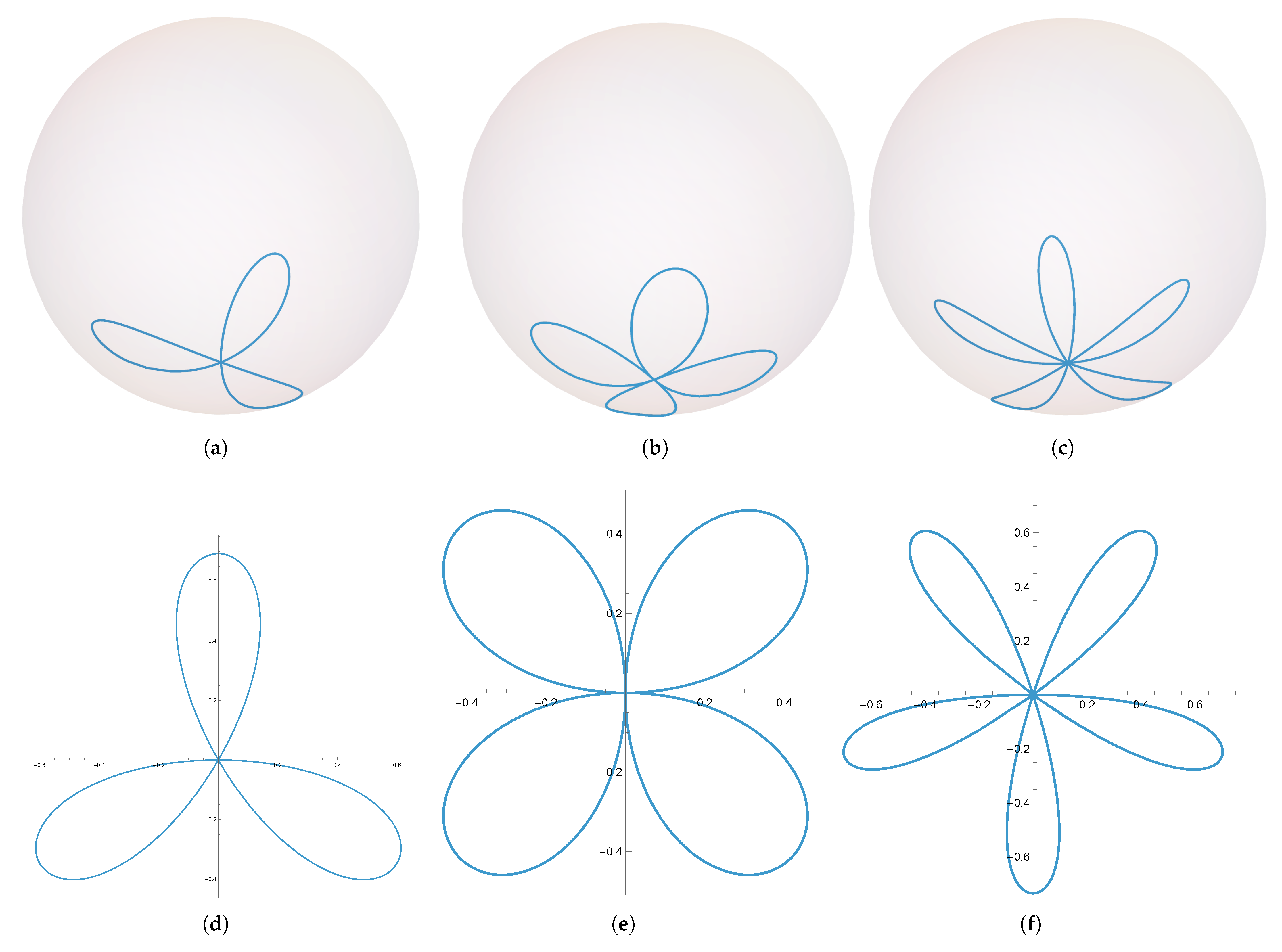
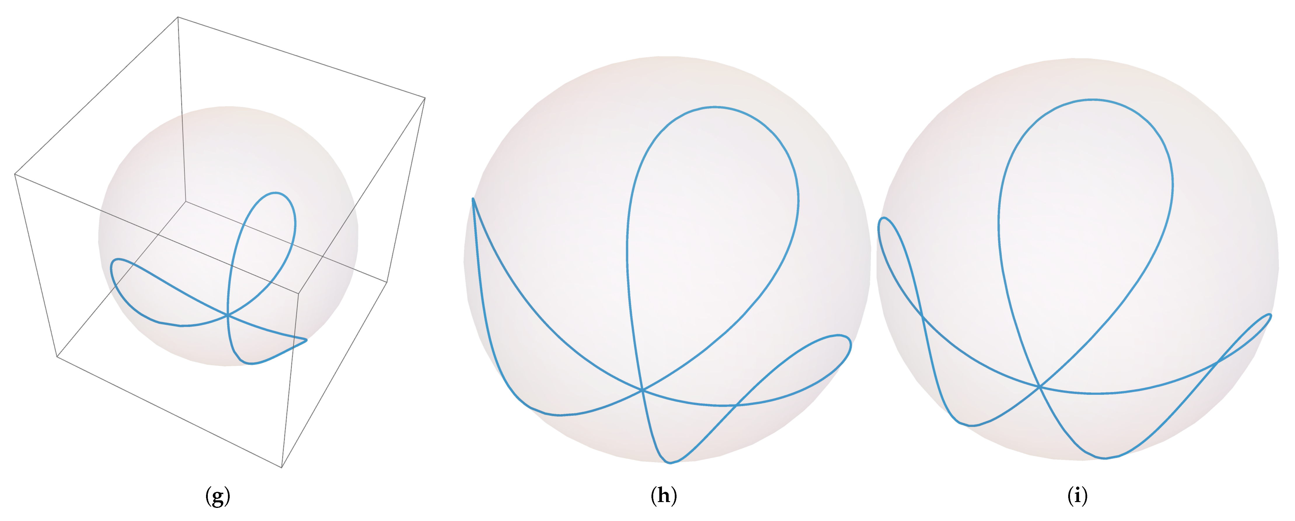
where $b=b(q,\rho )$ is given by Equation (7) and $z=z(s,q,\rho )$ is given by Equations (3) and (9). A solution curve with n leaves is determined by solving the equation $▵\theta (q,\rho )={\displaystyle \frac{2\pi }{n}}$. An example with $\rho =1\le k\le q=1.5125430973168356$ is shown in Figure 1.

3. Results

The z coordinate of a buckled ring is given explicitly in terms of the Jacobi elliptic cosine. The $\theta$ coordinate cannot in general be given in a closed form, but it can be found by one quadrature. Since Mathematica 14 has built-in routines for Jacobi elliptic functions, we are able to determine the precise values of the parameters corresponding to closed-curve solutions such as the one shown in Figure 1.

Numerical investigations establish the existence of three-leaf buckled spherical rings for a significant range of values of $\rho$. These curves are the spherical counterparts of the Kiepert trefoil, a buckled ring in the plane. In the planar case, such buckled rings are all related by similarity. Of course, no such relation can exist on the sphere. Even allowing the curvature $\rho$ at the vertex to be slightly negative results in such a curve. Figure 2 shows some examples of buckled rings.

For a given choice of the minimum curvature $\rho$ of the buckled ring, we may find the precise values of the maximum curvature q corresponding to solutions with n leaves. The following

Table 1. Examples of parameter values for closed curves.

$\mathit{\rho }$	q	Number of Leaves
1.2455061500613556	1	4
1.4263123428252	1	3
1.5125430973168356	1	8
1.56315419238342057	1	5
1.29893522750021006565	0.5	3
1.4768833847622324	0.01	3
1.4846434986989393	0	3

gives some representative examples of such parameters.

4. Discussion

Buckled rings can be thought of as being created from closed curves of a fixed perimeter containing a fixed area, which minimize bending energy while subject to uniform external pressure. When the pressure is very great, the curves are known to buckle into curves with n-fold dihedral symmetry. The curves studied in this article may be thought of as limit curves of this process, in which the curves make self-contact at a central point. While these may not be physically achievable, the curves are nevertheless natural as mathematical limits. Indeed, curves with multiple self-crossings, which would require the curve to pass through itself, are still solutions to the buckled ring equation. (Examples may be found in [3,7], Figure 9). From the point of view of soliton theory, all closed-curve solutions are of interest.

The goal of this research has been to establish the existence of a family of such limit curves in the case where the ambient space has positive curvature. A natural extension of this to the case of negative ambient curvature is an area for future research.