A Comparative Analysis of Three Data Fusion Methods and Construction of the Fusion Method Selection Paradigm

Abstract

Multisource and multimodal data fusion plays a pivotal role in large-scale artificial intelligence applications involving big data. However, the choice of fusion strategies for different scenarios is often based on experimental comparisons, which leads to increased computational costs during model training and suboptimal performance during testing. In this paper, we present a theoretical analysis of early fusion, late fusion, and gradual fusion methods. We derive equivalence conditions between early and late fusions within the framework of generalized linear models. Moreover, we analyze the failure conditions of early fusion in the presence of nonlinear feature-label relationships. Furthermore, we propose an approximate equation for evaluating the accuracy of early and late fusion methods as a function of sample size, feature quantity, and modality number. We also propose a critical sample size threshold at which the performance dominance of early fusion and late fusion models undergoes a reversal. Finally, we introduce a fusion method selection paradigm for selecting the most appropriate fusion method prior to task execution and demonstrate its effectiveness through extensive numerical experiments. Our theoretical framework is expected to solve the problems of computational and resource costs in model construction, improving the scalability and efficiency of data fusion methods.

1. Introduction

The ongoing advancement of data acquisition technologies has precipitated a proliferation of multimodal data representation paradigms for characterizing complex phenomena. In the pursuit of enhanced representational completeness, modern analytical frameworks increasingly incorporate advanced data fusion methods to synthesize disparate information sources. The data fusion method was first proposed and widely used by the US military, which was defined as “ multi-level process dealing with the association, correlation, combination of data and information from single and multiple sources to achieve refined position, identify estimates and complete and timely assessments of situations, threats and their significance” [1].

Since then, many scholars have classified data fusion methods. Durrant-Whyte classified data fusion methods into three categories, namely methods for complementarity data sources, redundancy data sources, and cooperation data sources [2]. In Dasarathy’s classification framework, data fusion techniques were systematically organized into a tripartite structure comprising signal fusion, feature fusion, and decision fusion, with this categorization predicated on the nature of input–output data modalities and their corresponding feature attributes [3]. At present, the mainstream classifications are mainly early fusion (EF), intermediate fusion (IF), and late fusion (LF) [4,5]. Early fusion, also known as data layer fusion, refers to the simple concatenation of original features as the input of a predictive classifier. Intermediate fusion, also known as feature layer fusion, refers to the learning of edge features of original data and the fusion of features for predictive classification. Late fusion, also known as decision layer fusion, refers to the training of unimodal models with different data and the fusion of model decisions [6,7,8]. Figure 1 shows the framework of these three types of data fusion methods. Comparative analysis of various data fusion methods has become a prominent focus in contemporary data fusion research.

At present, most studies on the comparative analysis of data fusion methods rely on experimental results from specific data sets, such as the comparison of the effect of early fusion and late fusion [9,10,11,12], early fusion and intermediate fusion [13,14,15], and the comprehensive comparison between the three fusion methods [16,17,18,19,20,21,22]. Few studies have compared the effects of different fusion methods based on the mechanism of different fusion methods. Pereira et al. [23], assuming a perfect model and a sufficiently large sample size, mathematically derived that early fusion outperforms late fusion in binary classification problems. What is more, an aspect worth thinking about is the lack of selection mechanism of fusion methods before performing predictive and classification tasks.

In this paper, we address the binary classification problem within the framework of data fusion. Specifically, we provide mathematical formulations for both early fusion and late fusion methodologies. Furthermore, we derive a mathematical definition of gradual fusion (GF) as a novel intermediate fusion approach, which processes data in a hierarchical, stepwise manner for prediction tasks [4,5]. In order to construct a fusion method selection paradigm, we first compare three fusion methods from the perspective of fusion mechanism and obtain the equivalent conditions of the early fusion and late fusion, the failure conditions of the early fusion when there is a gradual association between different features, and labels under the generalized linear model through mathematical derivation. Then, we propose an equation to evaluate the accuracy of the early fusion and late fusion by sample size, feature number, and mode number, and evaluate the critical sample size threshold at which the performance dominance of early fusion and late fusion models undergoes a reversal. Finally, based on the proposed equation, we give a discriminant paradigm that provides a theoretical basis for selecting fusion models before performing a specific task. The process of constructing the fusion method selection paradigm is shown in Figure 2.

The paper is structured in the following manner. In Section 2, the research questions and concepts related to data fusion are described. In Section 3, three fusion methods are compared and analyzed, and the fusion method selection paradigm is proposed. Then, the main conclusions are illustrated in Section 4 with examples. Finally, we discuss the work of this paper in detail and discuss the feasible research direction in the future.

2. Description of the Problem and Related Concepts

Since we are concerned with the fusion of multimodal data, any tasks related to data preprocessing are outside the scope of this article. We assume that the data have been filtered by the relevant variables, so all features have a prediction weight of non-0 relative to the label. In this paper, the mode features are denoted as ${\left\{X^i\right\}}_{i=1}^K$, $X^i=(x_1^i,x_2^i,...,x_{m_i}^i)$. $K$ represents the number of modes. The complete set of features was denoted as $X=(x_1,...,x_m)$, that is $\bigcup _{i=1}^K{X}_i=X$. We assume that none of the modes contain the cross-terms of the features, and the prediction models were all generalized linear models.

The generalized linear model is an extension of the classical linear regression model, which is capable of handling non-normally distributed response variables and allows the relationship between the linear predictor and the expected value of the response variable to be established through the link function. It is defined as follows [24].

Definition 1.

Suppose that the dependent variable ${Y=(Y}_1,Y_2,...,Y_n)$ obtains $n$ independent observations and follows an exponential distribution, i.e., there is a density function:

$$f(Y|\theta ,\varphi )=exp((Y\theta -b(\theta ))/\varphi +c(Y,\varphi )),$$

(1)

where $\theta$, $\varphi$ are the parameters, and $b(·)$ and $c(·)$ are the functions. When $\theta =K(X^T\beta )$, in which $X=(x_1,...,x_m)$ is the observed value of p-independent variable corresponding to the  $Y$, $\beta$ is the $p\times 1$ coefficient vector, and the function $K(·)$ describes the association between the independent variable $X$ and the parameter $\theta$. If there is a monotone differentiable connection function, such that

$$g(\mu )=\eta ={\mathrm{X}}^{\mathrm{T}}\beta ,$$

(2)

$$E(Y)=\mu ,$$

(3)

the model is called a generalized linear model. The inverse function of the join function $g^{-1}(·)$ is called the response function. Since the dependent variable $Y$ follows the exponential distribution, it can be calculated by the expectation of the exponential distribution that $E(Y)=b^{\prime }(\theta )=b^{\prime }(K(X^T\beta ))=F(X)$. So, the key to a generalized linear model is to find a monotone differentiable connection function $g(·)$ such that $g\circ F(X)=X^T\beta$. Since $g(·)$ is monotonic and differentiable, it is monotonic for every $x_i$ in $X$.

In early fusion, all features are spliced into a vector that serves as a unimodal input to the subsequent prediction model [25]. Therefore, the definition of early fusion can be given as follows.

Definition 2.

Given features of $K$ modes, the model that satisfies the following form is called the early fusion:

$$g_E\left(\mu \right)={\eta }_E=\sum _{i=1}^m{w}_i{x}_i,$$

(4)

where $g_E(·)$ is the connection function of the generalized linear model in the early fusion, ${\eta }_E$ is the output, $w_i$ is the weight coefficient ($w_i\ne$ 0), and the final prediction result is  $g_E^{-1}({\eta }_E)$.

In the late fusion, a separate model is trained for each mode, and the predictions from the individual models are aggregated to make the final prediction [4]. Therefore, the definition of late fusion can be given as follows.

Definition 3.

Given features of $K$ modes, the model that satisfies the following form is called the late fusion:

$$g_L^k(\mu )={\eta }_L^k={\sum }_{j=1}^{m_k}{w}_j^k{x}_j^k, k=\mathrm{1,2},...,K, x_j^k\in X,$$

(5)

$${output}_L=f({g_L^1}^{-1}({\eta }_L^1),{g_L^2}^{-1}({\eta }_L^2),...,{g_L^K}^{-1}({\eta }_L^K)),$$

(6)

where $g_L^k(·)$($k=\mathrm{1,2},...,K$) is the sub-model trained on the features of the $k$-th mode, ${g_L^k}^{-1}({\eta }_L^k)$ is the output, $f(·)$ is the fusion function of the decision, and ${output}_L$ is the final decision.

Gradual fusion is different from early fusion and late fusion. In this case, the features of different modes are fused step by step according to the correlation between modes. The mode with high correlation is fused first, while the mode with low correlation is fused later [4,5]. For gradual fusion, we can use a network diagram composed of modal and fusion functions to represent it.

Definition 4.

Given features of $K$ modes, the model that satisfies the following form is called the gradual fusion:

$$g_G(\mu )={\eta }_G=G(\overline{X},F),$$

(7)

where $\overline{X}$ represents the set of all modal features, $F$ represents the set of fusion prediction functions, the prediction function includes the input relations between modes and functions, and, therefore, $G$ represents the progressive fusion model graph of a whole composed of $\overline{X}$ and $F$.

Because the fusion functions are generalized linear models, the elements in $F$, as the output of the fusion prediction function, represent the inverse function of the connection function in the generalized linear model. The starting point of the directed connected edge in the network is the input of the end point, and there is a fusion function node with only the input degree and no output degree, that is, the final fusion prediction function, denoted as $f$. From (7), it is not difficult to achieve $f=g_G^{-1}(·)$. In addition, every modal node in the network must have a path to the final fusion prediction function node. See Appendix A for the detailed framework of the gradual fusion model construction.

Example 1.

Giving a case with 5 modal features ${\{X_i\}}_{i=1}^5$ and 4 fusion prediction functions  $\{f_1,f_2,f_3,f\}$. In first fusion step, $X_1$  and  $X_2$  are fused by $f_1$, while $X_3$  and  $X_4$  are fused by $f_2$. In the second fusion step, the results of $f_1$  and  $f_2$  are fused by $f_3$. Finally, the $X_5$  and the result of  $f_3$  are fused by $f$. The model can be represented as (8):

$$g_G\left(\mu \right)={\eta }_G=f\left(X_5,f_3\left(f_1\left(X_1,X_2\right),f_2\left(X_3,X_4\right)\right)\right).$$

(8)

3. Comparative Analysis and Construction of the Fusion Method Selection Paradigm

3.1. Comparative Analysis of Early Fusion and Late Fusion

Since the features have been variably filtered, we assume that for $\forall x_i,\exists {\eta }_i$, we include non-0 terms of $x_i$ and $w_j^i\ne$ 0. To start with the simple case, we consider $f(·)$ the case of a linear function in late fusion. According to the definitions of early fusion and late fusion, we find that the two methods may be equivalent in form, so let

$${\sum }_{k=1}^K{\alpha }_k{\eta }_L^k={\eta }_E.$$

(9)

When we bring (4), (5), (6) into Formula (9), we obtain

$${\sum }_{k=1}^K{\alpha }_k{\sum }_{j=1}^{m_k}{w}_j^k{x}_j^k={\sum }_{i=1}^m{w}_i{x}_i.$$

(10)

When Formula (10) is merged and sorted by $x$, we obtain

$${\sum }_{i=1}^m{x}_i{\sum }_{k=1}^K{\overline{w}}_k^i{\alpha }_k={\sum }_{i=1}^m{w}_i{x}_i,$$

(11)

where ${\overline{w}}_k^i$ is the coefficient of $x_i$ in Formula (5). A system of linear equations with respect to ${\alpha }_k$ is obtained by matching the coefficients of $x_i$.

$$\left\{\begin{array}{c}{\sum }_{k=1}^K{\overline{w}}_k^1{\alpha }_k=w_1\\ ⋮\\ {\sum }_{k=1}^K{\overline{w}}_k^m{\alpha }_k=w_m\end{array}\right.$$

(12)

Lemma 1.

Consistency Theorem for Nonhomogeneous Linear Systems [26]

$$\left\{\begin{array}{c}{a}_{11}{x}_1+a_{12}{x}_2+...+a_{1n}{x}_n=b_1\\ a_{21}{x}_1+a_{22}{x}_2+...+a_{2n}{x}_n=b_2\\ ⋮\\ a_{m1}{x}_1+a_{m2}{x}_1+...+a_{mn}{x}_n=b_m\end{array}\right.$$

(13)

The sufficient and necessary conditions governing the existence of solutions for the above equations are $r(A)=r(\tilde{A})$, where $A$ is the coefficient matrix of (13), $\tilde{A}$ is the augmented matrix of (13), and  $r(·)$ represents the rank of matrix.

Proof. 

See Appendix B for proof. □

According to Lemma 1, Equation (12) has a solution when the rank of the coefficient matrix $A$ is equal to the augmented matrix $\tilde{A}$. Let us assume that one of the solutions is $(\overline{{\alpha }_1},\overline{{\alpha }_2},...,\overline{{\alpha }_n}$), then $\sum _{k=1}^K\overline{{\alpha }_k}{\eta }_L^k={\eta }_E$. We only need to specify $f$ in Formula (6) to make the early fusion and the late fusion achieve the same output.

Theorem 1.

Under the condition of the generalized linear model, the necessary condition for the equivalence of early fusion and late fusion is that the rank of the coefficient matrix $A=\left({\overline{w}}_1,{\overline{w}}_2,...,{\overline{w}}_K\right)$ is equal to $\tilde{A}=\left({\overline{w}}_1,{\overline{w}}_2,...,{\overline{w}}_K,w\right)$, where ${\overline{w}}_i={(\begin{array}{ccc}{\overline{w}}_i^1& \cdots & {\overline{w}}_i^m\end{array})}^T (i=\mathrm{1,2},...,K)$ is the coefficient in the $i$-th sub-model of late fusion, and $w={(\begin{array}{ccc}{w}_1& \cdots & w_m\end{array})}^T$ is the coefficient of $x_i$ in the early fusion.

Proof. 

Because $r(A)=r(\tilde{A})$, according to Lemma 1, we can obtain $(\overline{{\alpha }_1},\overline{{\alpha }_2},...,\overline{{\alpha }_n}$), such that $\sum _{k=1}^K\overline{{\alpha }_k}{\eta }_L^k={\eta }_E$. In the late fusion model, outputs of sub-models are ${g_L^k}^{-1}({\eta }_L^k)$, which can be converted to ${\eta }_L^k$ by $g_L^k(·)$. So, we can set

$$f\left({g_L^1}^{-1}\left({\eta }_L^1\right),{g_L^2}^{-1}\left({\eta }_L^2\right),...,{g_L^K}^{-1}\left({\eta }_L^K\right)\right)=g_E^{-1}\left(\sum _{k=1}^K\overline{{\alpha }_k}{g}_L^k\left({g_L^k}^{-1}\left({\eta }_L^k\right)\right)\right).$$

(14)

Then, ${output}_{EF}={output}_{LF}$. The early fusion model and the late fusion model map the same input to the same output, which indicates the equivalence of the two models. □

Furthermore, we find that the number of equations in (12) represents the number of features, while $K$ represents the number of later fusion neutron models. We know that when the number of linearly independent equations in the system is greater than the number of unknowns, the system has no solution, so we can derive the following inference.

Inference 1.

When the number of linearly independent sub-models in the late fusion is less than the total number of features, the early fusion and the late fusion are not equivalent.

According to the conclusion of Theorem 1, we can also find that the early fusion is the parameter search on the full feature space, while the late fusion is the parameter search on the subspace of several features after incorporating the prior knowledge of feature grouping. In general, this kind of feature grouping is a lossy compression. Only when the feature grouping is accurate can the late fusion effectively reduce the parameter search space and improve the parameter search efficiency. This can be explained in detail by the information entropy theory. See Appendix A for details.

This provides us with a revelation that when the sample size is large enough, the model accuracy of the early fusion may be higher than that of the late fusion; however, the cost of sample sizes can be significant. In general, for a generalized linear model, when the number of linearly independent features is greater than the number of samples, the model will almost be overfit with probability 1. Therefore, in the early fusion, since the input of the model is the union of all modal features, the number of features will be very large, the requirements on the number of samples will be very high, and the total number of irrelevant features greater than that of all modes will be needed to greatly reduce the risk of overfitting. In the late fusion, because each mode is trained separately, the number of samples only needs to be greater than the largest number of irrelevant features in all modes, which greatly reduces the demand for the sample size. This conclusion is illustrated by the Vapnik–Chervonenkis (VC) dimension and the Hoeffding inequality [27,28].

When training generalized linear classifiers, there are empirical errors $E_{in}$ and generalization errors $E_{out}$. The training goal is to make empirical errors and generalization errors equal as much as possible. Through Hoeffding inequality, we can obtain the following formula [29]:

$$p(|E_{in}-E_{out}|>\epsilon )\le 4{(2N)}^{dvc}exp(-{\epsilon }^{2}N/8),$$

(15)

where $N$ represents the sample size and $dvc$ represents the VC dimension of the classifier. Since the VC dimension of the generalized linear classifier in the d-dimensional space is $d+1$, $dvc$ can be approximated as the feature dimension $d$. Derivation of right of Formula (14), with respect to the number of samples $N,$ is obtained as follows:

$$2{(2N)}^{d-1}(d-{\epsilon }^{2}N/8)exp(-{\epsilon }^{2}N/8).$$

(16)

Let (15) equal to 0, so that we can obtain $N=8d/{\epsilon }^2$. Therefore, when the sample size is large enough, with the increase in the sample size, the probability of $E_{in}=E_{out}$ is greater. However, when the number of features increases, in order to ensure the probability, the number of samples must also increase. In the early fusion, when the feature dimension increases $\Delta d_E$, the sample size needs to increase ${\displaystyle \frac{8\Delta d_E}{{\epsilon }^2}}$ as well. At this time in the late fusion, the increase in the feature dimension is $\Delta d_L\le \Delta d_E$, and, therefore, the increase in the sample size is $8\Delta d_L/{\epsilon }^2\le 8\Delta d_E/{\epsilon }^2$.

3.2. Comparative Analysis of Early Fusion and Gradual Fusion

In practical applications, the relationships between features and labels frequently exhibit significant complexity, often characterized by progressive associations. Such patterns are particularly prevalent in medical domains, where the diagnosis and treatment of diseases typically involve multifaceted interactions between clinical indicators and pathological outcomes [30,31]. Under such circumstances, conventional early fusion approaches may exhibit limited capacity to capture the intricate relationships inherent in the data, consequently leading to sub-optimal model performance in terms of predictive accuracy. We illustrate this by the following theorem.

Theorem 2.

Under the condition of generalized linear model, when there is a common feature $x$ among the modes, a common node in the path from the different modes contains $x$ to the final fusion prediction function. The fusion function of the common node is not monotonic for the features $x$. Then, the early fusion and gradual fusion are not equivalent.

Proof. 

According to the theorem conditions, we assume that $X_i\cap X_j=\{x\}$. It is obvious that there must be common nodes in the path from the different modes containing $x$ to the final fusion prediction function; at least the final fusion prediction function is one of them. Then, we assume that the fusion prediction function on this common node has the following expression for $X_i$ and $X_j$:

$$\tilde{\eta }=\tilde{f}(f_i(X_i),f_j(X_j))=w_i{f}_i(X_i)+w_j{f}_j(X_j)+C,$$

(17)

where $\tilde{f}$ represents the fusion prediction function represented by the common node, and $f_i$ and $f_j$ represent the fusion prediction function represented by the node pointing to $\tilde{f}$, respectively. We treat other modal features as constants, except for $X_i$ and $X_j$. According to the theorem condition, the pair is non-monotonic in the current node state. Since the fusion prediction functions on the path are all monotonic functions, the final fusion prediction function pair is also non-monotonic for $x$, so $f=g_G^{-1}(·)$ is non-monotonic for $x$. Suppose there are two multimodal feature sets ${\overline{X}}^1$ and ${\overline{X}}^2$, of which only feature x has different values, $x^1$ and $x^2$, respectively, $x^1{\ne x}^2$. In the gradual fusion model, ${\eta }_G^1=G({\overline{X}}^1, F)$ and ${\eta }_G^2=G({\overline{X}}^2, F)$, due to $g_G^{-1}\left(·\right),$ is non-monotonic for $x$, so we may as well assume that $g_G^{-1}({\eta }_G^1)=g_G^{-1}({\eta }_G^2)$. In the early fusion model, ${\eta }_E^1=W{\overline{X}}^1=\sum _{i=1}^{m-1}{w}_i{x}_i+w{x}^1$ and ${\eta }_E^2=W{\overline{X}}^2=\sum _{i=1}^{m-1}{w}_i{x}_i+w{x}^2$, then ${\eta }_E^1\ne {\eta }_E^2$, so $g_E^{-1}({\eta }_E^1)\ne g_E^{-1}({\eta }_E^2)$. This situation shows that gradual fusion maps ${\overline{X}}^1$ and ${\overline{X}}^2$ to the same output, while the early fusion maps the two data sets to different outputs, so the gradual fusion model and the early fusion model are non-equivalent. Proof over. □

To illustrate the content of Theorem 2, let us take a concrete example.

Example 2.

There are three modes of features. Each mode includes three-dimensional features denoted as $X_1=(x_1^1,x_2^1,x_3^1)$,  $X_2=(x_1^2,x_2^2,x_3^2)$, and $X_3=(x_1^1,x_2^3,x_3^3)$. In constructing the gradual fusion model, $X_1$ and $X_2$ are fused first, and then $X_3$ is fused. The prediction model used is the Logistic model. Suppose the expression for the fusion of $X_1$ and $X_2$ is ${\eta }_1=\sum _{i=1}^2\sum _{x_j^k\in X_i}{x}_j^k$. The fusion feature after the first fusion is

$$1/(1+exp(-({\sum }_{i=1}^2{\sum }_{x_j^k\in X_i}{x}_j^k))).$$

(18)

Let the fusion feature after the second fusion be

$$1/(1+exp(-({\sum }_{i=1}^2{\sum }_{x_j^k\in X_i}{x}_j^k)))-x_1^1/5+x_2^3+x_3^3.$$

(19)

Then, the prediction expression after the second fusion is

$$g_G(\mu )={\eta }_G=1/(1+exp(-({\sum }_{i=1}^2{\sum }_{x_j^k\in X_i}{x}_j^k)))-x_1^1/5+x_2^3+x_3^3.$$

(20)

We can obtain

$${\displaystyle \frac{\partial g_G(\mu )}{\partial x_1^1}}=exp(-({\sum }_{i=1}^2{\sum }_{x_j^k\in X_i}{x}_j^k))/(1+exp(-({\sum }_{i=1}^2{\sum }_{x_j^k\in X_i}{x}_j^k))))-1/5.$$

(21)

Obviously, $\partial g_G(\mu )/\partial x_1^1$ is not constant positive or negative, so $g_G(·)$ is not monotonic for $x_1^1$. In this case, $g_G(·)$ is not a generalized linear model.

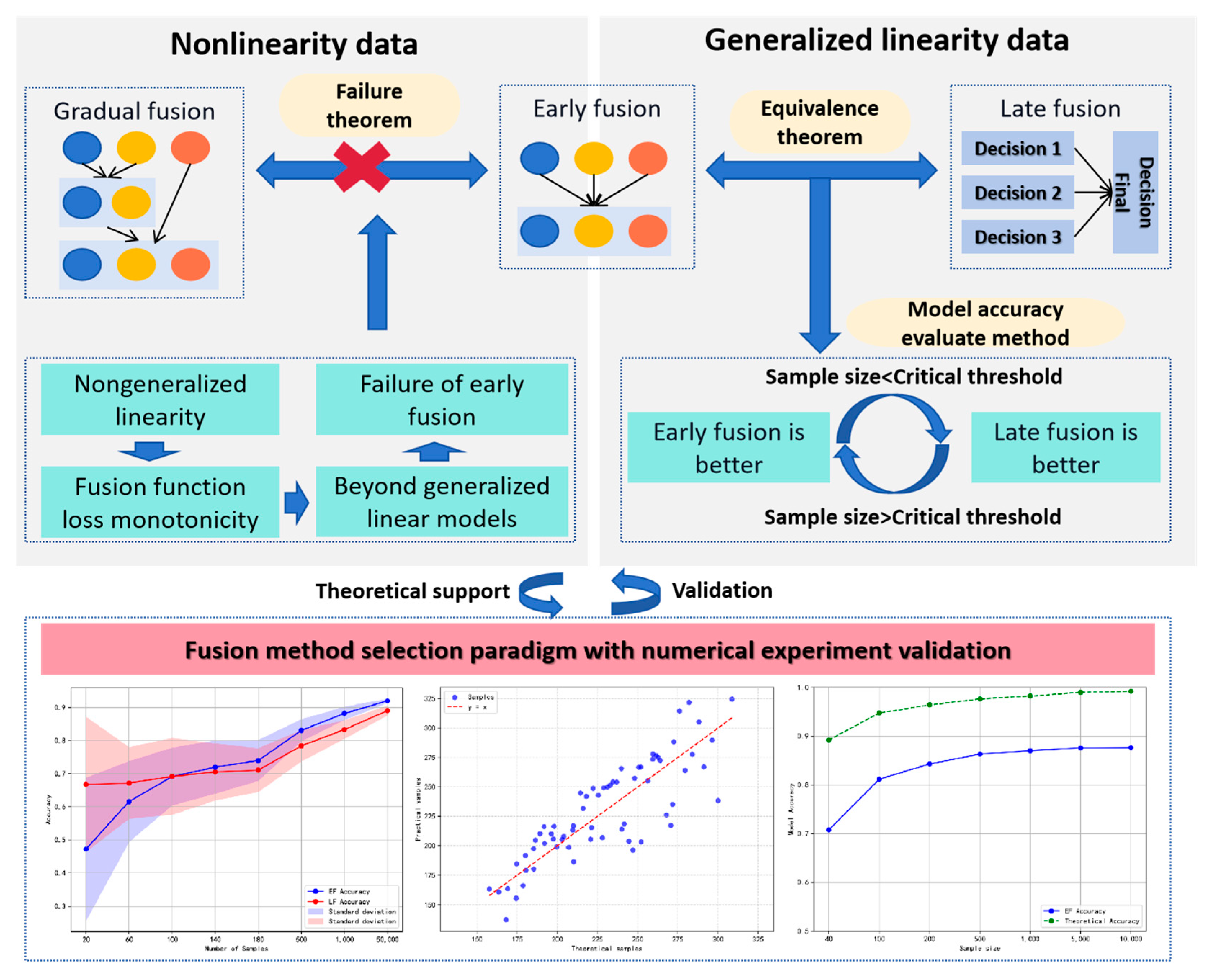
3.3. Construction of the Fusion Method Selection Paradigm

Theoretically, when there is a generalized linear relationship between the labels and each modal feature, the prediction accuracy of the early fusion model can approach 1 when the sample is large enough, while the accuracy of the later fusion model may approach $1-\epsilon$ due to the loss caused by the compression of the feature space. For this reason, we propose approximate Equations (21) and (22) to evaluate the early fusion and late fusion models’ accuracy through sample size, feature quantity, and modality number in early and late fusions. Furthermore, the suitability of early fusion and late fusion under varying sample size conditions is evaluated.

$${Accuracy}_{EF}=1-{\alpha }_1\ast d_{all}/N-{\alpha }_2\ast \sigma /\sqrt[3]{N},$$

(22)

$${Accuracy}_{LF}=1-{\alpha }_1\ast d_{max}/N-{\alpha }_2\ast \sigma /\sqrt[3]{N}-{\alpha }_3\ast \sqrt{K},$$

(23)

where $d_{all}$ represents the sum number of all features and $d_{max}$ represents the max number of all mode features. $d_{all}/N$ and $d_{max}/N$ represent the overfitting risk due to imbalance between the feature number and the sample number [32]. $\sigma /\sqrt[3]{N}$ represents uncertainty induced by data noise [33]. $\sqrt{K}$ represents parameter search loss due to modal partitioning. Data signal-to-noise ratio is calculated by (23):

$$\sigma =Var(\widehat{y})/Var(ϵ),$$

(24)

where $Var(\widehat{y})$ represents the variance of the predicted value by the linear regression model. $Var(ϵ)$ represents the variance of the residual difference between the predicted value and the true label predicted by the linear regression model. Through Equations (21) and (22), we calculate the sample critical value of early fusion and late fusion under the same set of data. Let ${Accuracy}_{EF}={Accuracy}_{LF}$, so we can obtain

$$N_{critical}={\alpha }_1(d_{all}-d_{max})/{\alpha }_3\ast \sqrt{K}.$$

(25)

When the sample size exceeds the threshold, the performance of the early fusion model outperforms that of the late fusion model.

According to Equations (21) and (22), a fusion method selection paradigm is proposed before constructing the prediction model.

(a)

Samples are randomly drawn from the population with a predetermined sample size range of $[d_{all}/3, 100d_{all}]$. For each sampled set, the signal-to-noise ratio is calculated simultaneously.

(b)

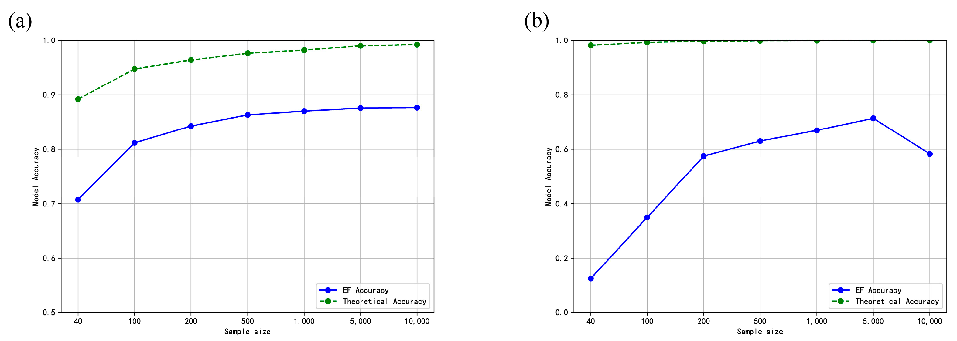
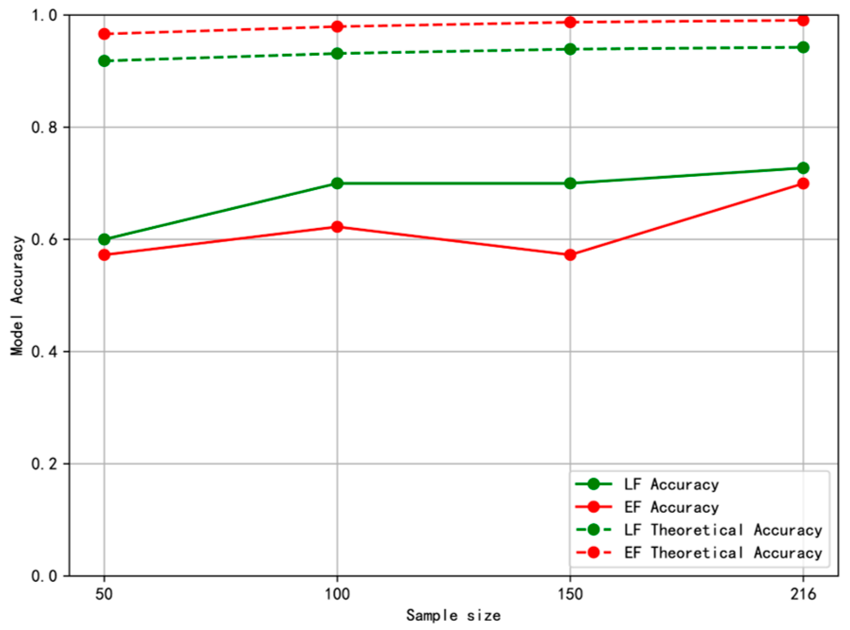
Generalized linear models are employed to construct both early fusion and late fusion models. The models are trained on the sampled datasets, and their predictive accuracy is systematically recorded. Concurrently, the theoretical accuracy under the given sample conditions is computed using Equations (21) and (22).

(c)

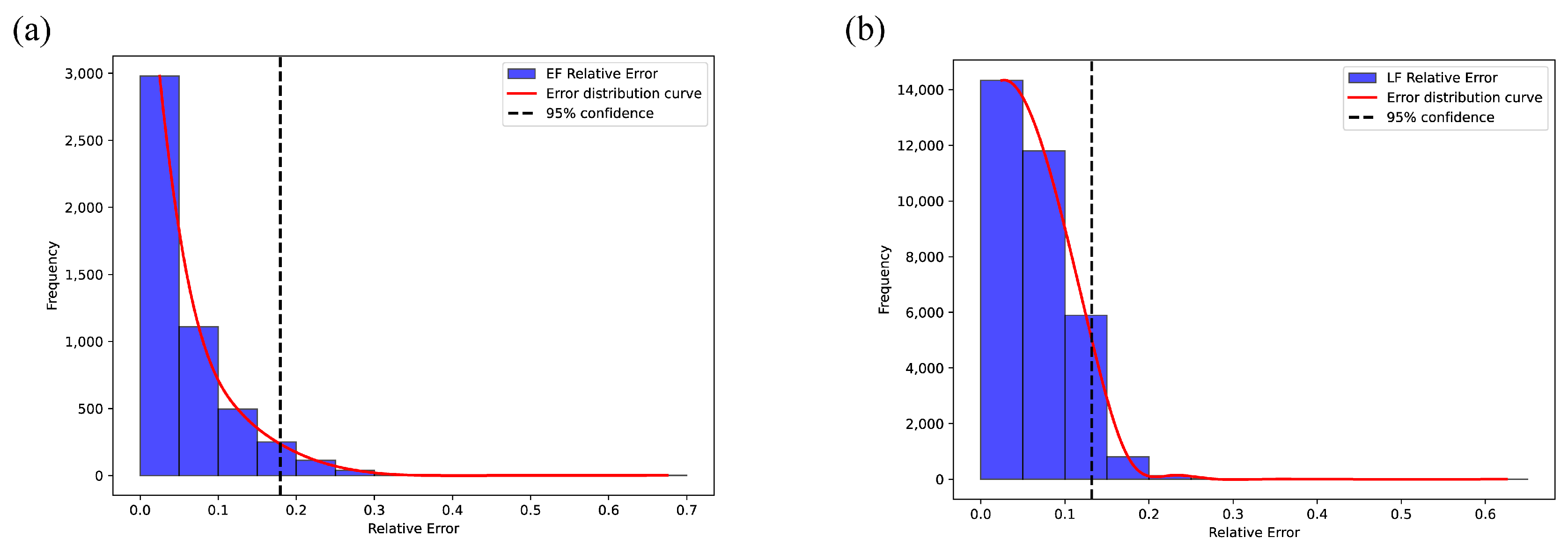
A comparative analysis is conducted between the empirical model’s accuracy and the theoretical accuracy. If the maximum deviation between the model’s accuracy and the theoretical accuracy for either early or late fusion does not exceed 20%, the task can be appropriately addressed using the corresponding generalized linear fusion approach. Conversely, if the deviation exceeds this threshold, the relationship between features and labels is deemed nonlinear, suggesting that generalized linear fusion methods (either early or late fusion) are insufficient. At a 95% confidence level, more sophisticated fusion strategies, such as progressive fusion, should be considered to capture the underlying complexity of the data.

4. Numerical Experiment Validation

4.1. Example of Early Fusion and Late Fusion Equivalence

Let the feature set be $X=(x_1,x_2,x_3)$, and there are three modes $X_1=(x_2,x_3)$, $X_2=(x_1,x_3)$ and $X_3=(x_1,x_2)$. Constructing a set of 1000 samples, $x_i(i=\mathrm{1,2},3)$ follows a uniform distribution between (0,1). $X_i(i=\mathrm{1,2},3)$ is constructed as described above. Then, a 2-dimensional weight vector between (0,1) is randomly generated for each one, and the average of the sum of the product of each modal feature and the weight is calculated. The final step involves substituting the mean value into the logistic function to compute the variable $\tilde{y}$. In order to simulate the binary classification scenario and make the two types of samples balance, the median is taken as the threshold of mapping $\tilde{y}$ to the binary value to obtain the final label $y$. The whole process is as follows:

$$\tilde{y}=1/(1+exp(-({\sum }_{i=1}^3{w}_i{X}_i)/3)),$$

(26)

$$y=\left\{\begin{array}{c}0, \tilde{y}\le median \\ 1, \tilde{y}>median\end{array}\right..$$

(27)

Using the above three modes to train the logistic regression model through early fusion and late fusion, respectively, the iteration steps of logistic regression model is 100. The expression of early fusion is as follows:

$$ln(y/(1-y))=5.688x_1+9.51x_2+9.142x_3.$$

(28)

The expressions of the three sub-models in the late fusion are as follows:

$$\left\{\begin{array}{c}ln(y/(1-y))=6.131x_2+6.02x_3\\ ln(y/(1-y))=2.846x_1+4.401x_3\\ ln(y/(1-y))=2.944x_1+4.655x_2\end{array}\right..$$

(29)

We can obtain the coefficient matrix $A$ and the augmented matrix $\tilde{A}$, $rank(A)=rank(\tilde{A})=3$. So, early fusion and late fusion are equivalent to Theorem 1. It can be further found that $({\alpha }_1,{\alpha }_2,{\alpha }_3)=(\mathrm{0.803,0.979,0.986})$ is a solution to the system. In the late fusion, the three sub-models can be mapped to the expression of the early fusion by summing the weights with linear weights.

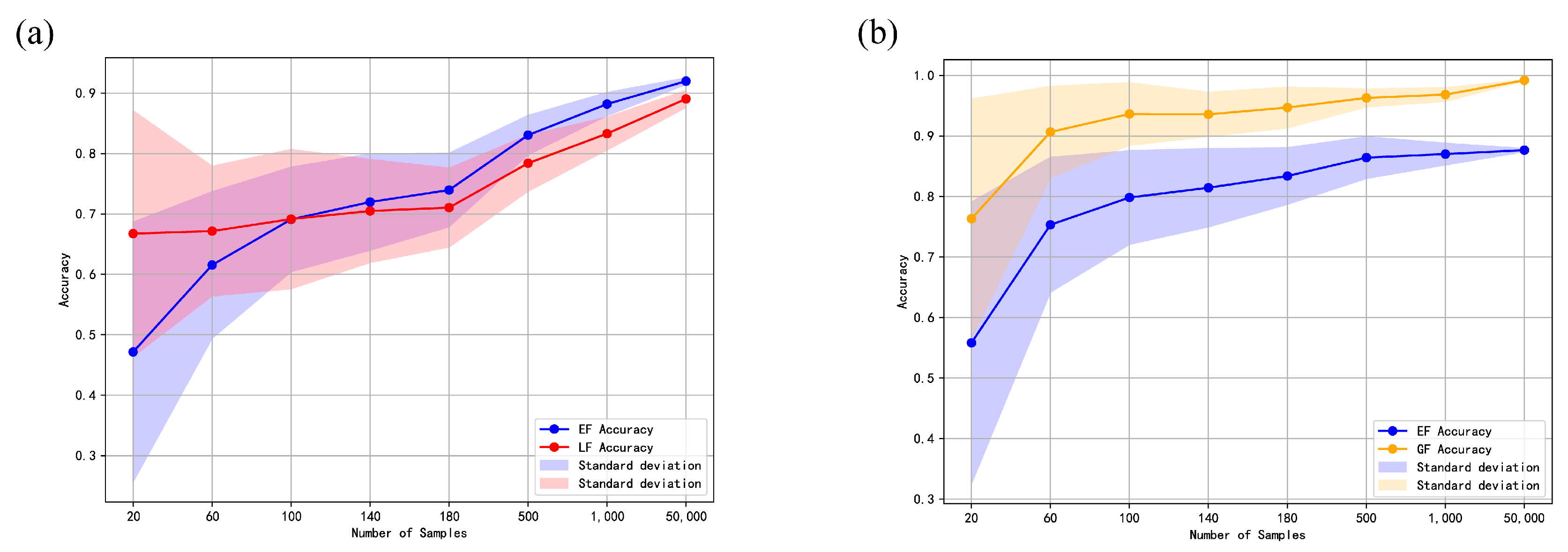
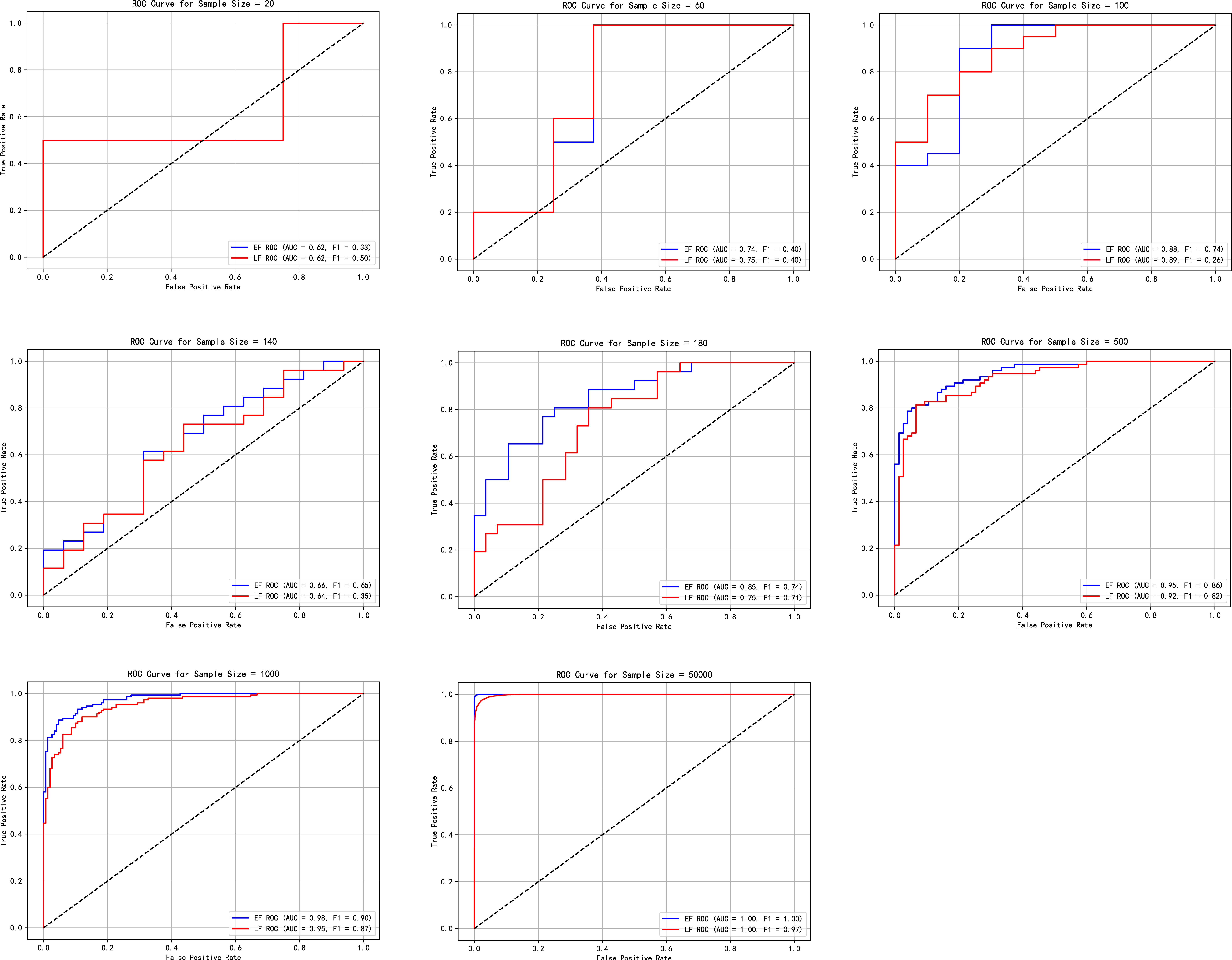
4.2. Comparative Experimental Analysis of Early Fusion and Late Fusion Models

Ten groups of 10-dimensional random variables between (0,1) are randomly generated as the features of the 10 modes, and the weight vector between (0,1) of the corresponding dimension is generated at the same time. The logical function values of the 10 modal features under the weights are calculated, respectively, and the obtained values are averaged and mapped to binary value as the label; see Algorithm 1 for details. The model is a logistic model and trained by early fusion and late fusion, respectively. The iteration steps of the logistic regression model is also 100. In early fusion, the features of all modes are spliced into a vector input model for training. In the late fusion, sub-model is trained on each mode, and the model output is linearly combined to obtain the final prediction result. The samples are divided into a training set and a test set in a 7:3 ratio. The experiment is repeated 100 times, and the average is used as the result.

Algorithm 1 Data Generation Algorithm of Late Fusion Mode

Random $W=\{w_1,w_2,...,w_{10}\}$, $w_j=(w_1^j,w_2^j,...,w_{10}^j)$

For i in Sample numbers:

Random $\{X_1^i,X_2^i,...,X_{10}^i\}$, $X_j^i=(x_1^j,x_2^j,...,x_{10}^j)$, $j,k=(\mathrm{1,2},...,10)$

Calculate $y_j^i=sigmoid(w_j·X_j^{iT})$

Calculate ${\overline{y}}^i=mean{\{y_j^i\}}_{j=1}^{10}$

$\overline{y}={({\overline{y}}^i)}_{i=1}^{\mathrm{S}\mathrm{a}\mathrm{m}\mathrm{p}\mathrm{l}\mathrm{e} \mathrm{n}\mathrm{u}\mathrm{m}\mathrm{b}\mathrm{e}\mathrm{r}\mathrm{s}}$

$\delta =median\{\overline{y}\}$

If ${\overline{y}}^i\ge \delta$:

${\overline{y}}^i=1$

Else:

${\overline{y}}^i=0$

Figure 3a shows the prediction accuracy of the two fusion methods. It can be found that the model accuracy of the two fusion methods increases with the increase in the number of samples. In addition, when the number of samples is small, due to the feature compression of late fusion, the search space becomes smaller so that the prediction accuracy of the model in late fusion is higher than that in the early fusion. When the sample is large enough, the search in the full feature space in the early fusion makes the model accuracy higher than that in the later fusion. It can also be found that with the continuous improvement of accuracy, the sample size required to increase the same accuracy is also increasing. Furthermore, we also compared the ROC curve and F1-score of the two fusion methods under different sample sizes, as shown in Figure 4. When the sample size is less than 100, the late fusion is better than the early fusion, and when the sample size is more than 100, the early fusion is better than the late fusion, which is consistent with the conclusion of the model’s accuracy.

4.3. Comparative Experimental Analysis of Early Fusion and Gradual Fusion Models

The gradual fusion model in this section consists of two stages. In the first stage, features from certain modalities are grouped, and pairwise dot product calculations are performed. In the second stage, the logarithmic values of computed pairwise values, along with the remaining modality features, are fused into a feature vector using the parallel splicing method from the previous fusion. This fused vector then serves as the input for the final prediction model. The specific experimental process is as follows.

Randomly generate four groups of three-dimensional random variables between (0,1) as features of the four modes. In particular, the last feature of the second and fourth modes is between (0,0.5). Then, the one-dimensional random variable between (0,1), the last feature of the first mode, and the third mode multiply by $-1/9$, which constitutes the feature of the fifth mode. Multiply the corresponding features of the first and second modes, as well as the third and fourth modes to calculate the logarithmic function value. The two pairs of the obtained values and the features of the fifth mode are calculated with the weight 1 to obtain the logical function value, and map it to the binary value as the label; see Algorithm 2 for details. It is obvious that label is non-monotonic for the last feature of the first mode and the third mode. In the early fusion training, the process is similar to the early fusion model training in Section 4.2. In gradual fusion, according to the process of data generation, the corresponding features of the first and second modes, the third and fourth modes are multiplied to obtain the pair value as the fusion feature of the first step. Then, the fusion feature and the features of the fifth mode are used to train the logistic regression model. The samples are divided into the training set and the test set in a 7:3 ratio. The experiment was repeated 100 times, and the average was used as the result.

Algorithm 2 Data Generation Algorithm of Gradual Fusion Mode

For i in Sample numbers:

Random $X_1^i=\{x_1^i,x_2^i,x_3^i\}$, $X_2^i=\{x_4^i,x_5^i,x_6^i\}$, $X_3^i=\{x_7^i,x_8^i,x_9^i\}$, $X_4^i=\{x_{10}^i,x_{11}^i,x_{12}^i\}$, $X_5^i=\{{-{\displaystyle \frac{1}{9}}{x}_3^i}_3,-{\displaystyle \frac{1}{9}}{x}_9^i,x_{13}^i\}$. $x_j^iϵ(\mathrm{0,1}) (j\ne \mathrm{6,12})$, $x_j^iϵ(\mathrm{0,0.5}) (j=\mathrm{6,12})$

Calculate $y_1^i=log(X_1^i·X_2^{iT})$ and $y_2^i=log(X_3^i·X_4^{iT})$

Calculate ${\overline{y}}^i=Sigmoid(y_1^i+y_2^i-x_3^i/9-x_9^i/9+x_{13}^i)$

$\overline{y}={({\overline{y}}^i)}_{i=1}^{\mathrm{S}\mathrm{a}\mathrm{m}\mathrm{p}\mathrm{l}\mathrm{e} \mathrm{n}\mathrm{u}\mathrm{m}\mathrm{b}\mathrm{e}\mathrm{r}\mathrm{s}}$

$\delta =median\{\overline{y}\}$

If ${\overline{y}}^i\ge \delta$:

${\overline{y}}^i=1$

Else:

${\overline{y}}^i=0$

Figure 3b shows the prediction results of the two fusion methods. It can be found that the gradual fusion is better than the early fusion overall. When the sample size is large enough, the accuracy of the gradual fusion model tends to be 1. When the sample size is small, the precision of the early fusion is low, and when the sample size is increased, the search effect of the full-feature space is enhanced but the upper bound is only 0.9, indicating that the gradual fusion method is worth considering when there is a nonlinear gradual relationship between the features and the labels. In the same way, we also compared the ROC curve and F1-score of the two fusion methods under different sample sizes, as shown in Figure 5. We can see that the effect of gradual fusion is better than that of early fusion in all cases of the sample size, which is consistent with the conclusion of model accuracy.

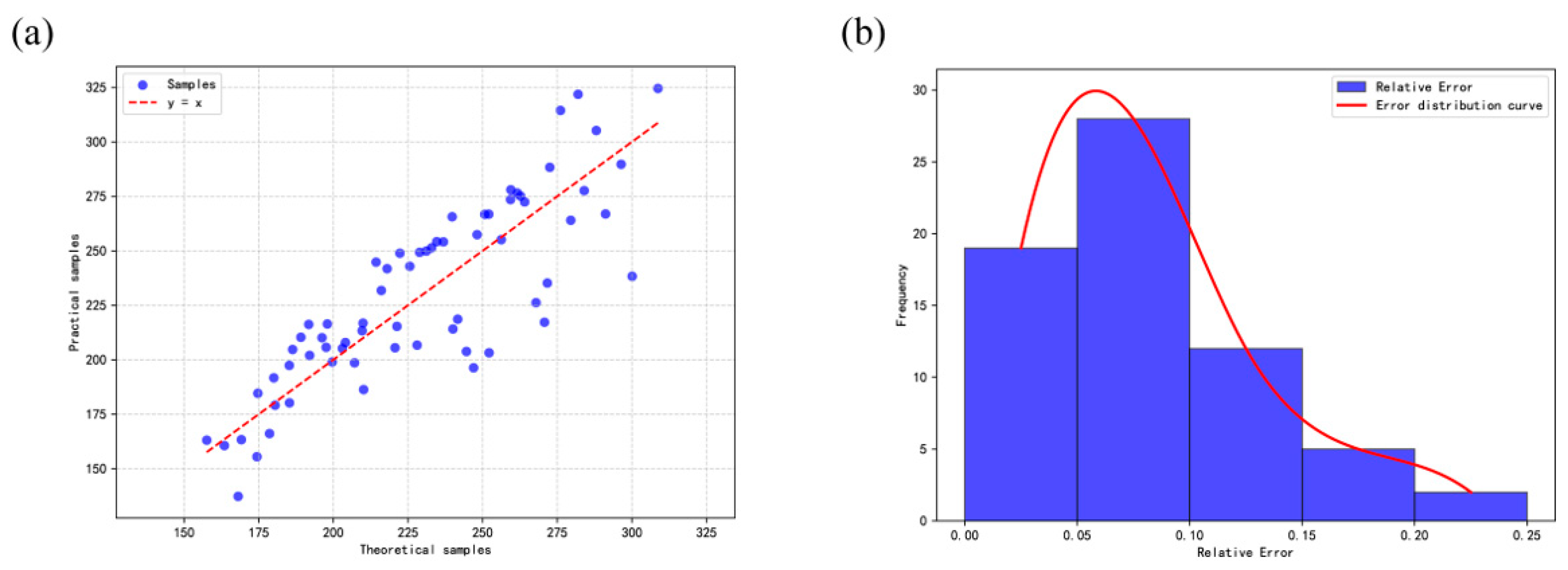
4.4. Effect Verification of the Approximate Equation and Method Selection Paradigm

In order to illustrate the validity of the accuracy evaluation’s equation form, we perform a series of numerical experiments under the model scene in this paper. First, we estimated the parameters in the equation by numerical experiments. We took $K\in \left[\mathrm{15,20}\right]$, $d_{max}\in \left[\mathrm{15,25}\right]$, and $d_{all}=K\ast d_{max}$ and conduct multiple sets of early and late fusion experiments. Each set of experiments was repeated 100 times to obtain the average value, and the estimate of the critical value of the actual sample was obtained by the method of mapping the intersection points of the experiments. The range of ${\alpha }_1$ and ${\alpha }_3$ were estimated experimentally by minimizing the mean square error of the theoretical and actual values and by grid search. In our experimental setup, the optimal values of ${\alpha }_1$ and ${\alpha }_3$ were 0.071 and 0.024, respectively. Figure 6a shows the distribution of the theoretical sample’s critical values and the actual sample’s critical values; it can be seen that the scattered points were basically around $y=x$. At the same time, Figure 6b shows the error distribution of the theoretical sample critical values and actual sample critical values, it can be seen that the errors of the theoretical sample’s critical values and the actual sample’s critical values were less than or equal to 0.25, and most of them were within 0.15.

Equations (36) and (37) in [23] also described the sample size $N_{EF}$ and $N_{LF}$ required for early fusion and late fusion, in which the convergence factor is 0.9. It indicates that the effect of the late fusion model may be better than that of the early fusion model when the sample size is between $N_{LF}$ and $N_{EF}$. We compared our calculated $N_{critical}$ with $N_{EF}$ and $N_{LF}$ in four typical cases. The experimental parameters and results are shown in

Table 1. The experimental parameters and results of sample size comparison experiment.

Experimental Parameters	${\mathbf{N}}_{\mathbf{a}\mathbf{c}\mathbf{t}\mathbf{u}\mathbf{a}\mathbf{l}}$	${\mathbf{N}}_{\mathbf{E}\mathbf{F}}$	${\mathbf{N}}_{\mathbf{L}\mathbf{F}}$	${\mathbf{N}}_{\mathbf{c}\mathbf{r}\mathbf{i}\mathbf{t}\mathbf{i}\mathbf{c}\mathbf{a}\mathbf{l}}$
$K=3$$, d_{max}=50$$, d_{all}=150$	185	1511	511	170
$K=15$$, d_{max}=10$$, d_{all}=150$	95	1511	111	106
$K=$$3, d_{max}=15$$0, d_{all}=450$	490	4511	1511	512
$K=$$15, d_{max}=$$30, d_{all}=450$	340	4511	311	320

. In [23], the sample sizes for early fusion and late fusion were evaluated under the premise of ensuring model accuracy, leading to a certain degree of redundancy in the sample estimates derived from parameters $N_{EF}$ and $N_{LF}$. More importantly, the study did not account for the correlation between the number of modes and the performance of the early fusion model. In contrast, our proposed method incorporates this factor, allowing our results to more precisely characterize the critical sample threshold at which the performance reversal between early fusion and late fusion models occurs.

Then, we perform the early fusion experiments in which the total number of features is a multiple of 10, the sample size is 200, 500, 1000, 5000, 10,000. Based on the grid search method of theoretical accuracy and model accuracy, we obtain the optimal ${\mathsf{\alpha }}_2$ is 0.033. Figure 7a shows the relative error between the actual accuracy of the model and the theoretical accuracy of all the early fusion experiments, and it can be seen that the relative error is about 0.18 with 95% confidence. Furthermore, we conducted a late fusion experiment in which the number of modes is integer between [15, 20] and the number of features of each mode is integer between [15, 25]. The sample sizes are also 200, 500, 1000, 5000, and 10,000. Figure 7b shows the relative error between the actual accuracy of the model and the theoretical accuracy of all experiments, and it can be seen that the error is about 0.14 with 95% confidence.

In order to verify the fusion method selection paradigm, Figure 8a shows the model accuracy and theoretical accuracy of the early fusion under the gradual fusion data, including five modes. It can be seen that when the sample size is small, the model accuracy of the early fusion is much different from the theoretical accuracy and the maximum error is about 21.1%. In addition, we also simulated the Lorentz system, a typical scenario in a group of nonlinear systems, and made predictions through the early fusion of logistic regression models. Figure 8b shows the accuracy of the model and its theoretical accuracy. The maximum error is far more than 20%, thus demonstrating the effectiveness of the proposed fusion method selection paradigm.

To reinforce the validation of the model selection paradigm, we applied our paradigm to a real data set of hypoproteinemia patients from a previous study [34]. The data set included 108 control patients and 108 experimental patients, each with four different medical examination features. According to the model selection paradigm, 50, 100, 150, and 216 samples were selected according to the equal proportion of labels to conduct early fusion model and late fusion model experiments. The accuracy of the theoretical model was also calculated, as shown in Figure 9. The results in the figure indicate that the maximum discrepancy between the actual model accuracy and the theoretical accuracy for both early fusion and late fusion exceeds 20%. This suggests that the applicability of these two models in this scenario is limited, thereby highlighting the effectiveness of our proposed model selection paradigm.

5. Discussion

The multisource and multimodal data fusion model has been widely used across various fields, but most of the research is still in the application level and the theoretical comparison of different data fusion methods is rarely studied. Since it is difficult to express all kinds of nonlinear models uniformly and the models themselves are complex, we consider a simple generalized linear model as a starting point for analysis. This paper analyzes the similarities and differences in the early fusion, late fusion, and gradual fusion from the perspective of fusion mechanism through mathematical derivation. Furthermore, a model accuracy evaluation equation is proposed in the early fusion and the late fusion, and the critical sample size threshold evaluates the method at which the performance dominance of early fusion and late fusion models that undergoes a reversal is analyzed. Finally, we give the selection evaluation paradigm of the fusion method in the construction of fusion model.

Specifically, we first give the mathematical definitions of early fusion and late fusion. Based on the definition, the unified expression of the generalized linear model is introduced for derivation. During the derivation process, we find that the equivalence of early fusion and late fusion depends on the model parameter, then the equivalence problem is transformed into a non-homogeneous linear system of model parameters. By the consistency theorem of the non-homogeneous linear system in linear algebra, we obtain the equivalence conditions of the earlier fusion and the later fusion. In the numerical experiment, we found that when the sample size was large, the effect of the early-stage fusion model was better than that of the late-stage fusion, even when the features and labels relatively met the mode of late-stage fusion. One possible reason is that in the early-stage fusion, parameter search is carried out in the full feature space, while in the later stage fusion, the features are divided into different modes for sub-model training, so the search space of parameters is compressed. If the modal distinction is not perfect, certain search loss will be caused, making the model unable to find the optimal parameter in the full space. This is consistent with the conclusion obtained by Pereira et al. [23]. Through a series of analysis, we highlight that under ideal conditions, specifically when the sample size is sufficiently large, there is no need for a complex late fusion. This is because the early fusion model can explore the entire parameter space to find the optimal solution, making it equivalent to or even superior to the late fusion model. However, in real-world scenarios, where sample sizes are often limited, early fusion tends to perform poorly. In such cases, late fusion can leverage its advantages to achieve an acceptable level of prediction accuracy.

We then give a mathematical definition of gradual fusion. We consider that the data features and labels meet the gradual fusion mode, so a nonlinear relationship is introduced between the features and labels. Based on the definition of the generalized linear model, we find that once the monotonicity between intermediate hidden variables and features is lost in the process of progressive fusion, the final label and features will no longer meet the definition of the generalized linear model, so the gradual fusion model and the early fusion will not be equivalent. This conclusion is also verified by numerical experiments.

Furthermore, we consider whether it is possible to quantify the correlation between the model accuracy and the data attributes of early fusion and late fusion. We assume that under the generalized linear condition, the association complexity between data features and labels is low, and combined with literature [19], we put forward Equations (21) and (22). Based on (21) and (22), we analyze the sample critical points of the model accuracy of early fusion and late fusion. Combined with numerical experiments of critical points, we give an estimate of the parameters through an optimization method. Moreover, the numerical experiment results show that the model relative error of the early fusion and the late fusion is controlled at about 18% and 14% with 95% confidence, which indicates the validity of Formulas (21) and (22). Finally, we put forward an evaluation paradigm for the selection of fusion mode in the construction of a fusion model, which provides a certain theoretical basis for the selection of fusion mode before model construction.

The research in this paper is carried out under the condition of the generalized linear model, and one of the future research directions is to extend the application scope of our conclusions to a specific class of nonlinear models, such as deep learning. Deep learning fundamentally relies on two key concepts: perceptrons and activation functions. By stacking multiple layers of perceptrons, activation functions, and various additional operations, a diverse range of deep learning models can be constructed. Since a perceptron combined with a sigmoid activation function essentially forms a generalized linear model, our findings can be extended to the design of single-layer perceptrons within certain deep-learning architectures, particularly in determining sample sizes and parameter counts. In addition, the parameter optimization of Formulas (21) and (22) is also a worthy research direction. Finding better parameters can narrow the error threshold in the selection evaluation paradigm of fusion mode and make the evaluation more accurate.

6. Conclusions

In this paper, we propose selection paradigms that provide a theoretical basis for selecting early fusion, late fusion, and gradual fusion models before performing a specific task. Unlike most of the recent fusion model studies that have on experimental results, our research is performed based on the mechanistic understanding of the fusion process. Specifically, we establish the equivalence conditions between early fusion and late fusion within the framework of generalized linear models, along with the failure conditions of early fusion in scenarios where nonlinear correlations exist between features and labels. This enhances our understanding of the similarities and differences between various fusion methods. Subsequently, we construct model accuracy evaluation equations that incorporate sample size, feature quantity, and modality number guided by theoretical insights, enabling a data-driven approach to fusion method evaluation. Furthermore, we propose a critical sample size threshold evaluation method at which the performance dominance of early fusion and late fusion models undergoes a reversal through the equations, allowing for the understanding of the trade-offs between model accuracy and data size. Finally, we propose the model selection paradigm based on accuracy evaluation equations. Numerical experimental results demonstrate that the proposed paradigm reliably identifies the optimal fusion strategy. In future research, our theoretical framework is anticipated to significantly reduce the computational and resource costs associated with model construction, thereby enhancing the scalability and efficiency of data fusion methodologies.

References

1. White, F.E. Data fusion lexicon. JDL. Tech. Panel C 1991, 3, 19. [Google Scholar]
2. Durrant-Whyte, H.F. Sensor models and multisensor integration. Int. J. Robot. Res. 1988, 7, 97–113. [Google Scholar] [CrossRef]
3. Dasarathy, B.V. Sensor fusion potential exploitation-innovative architectures and illustrative applications. Proc. IEEE 1997, 85, 24–38. [Google Scholar]
4. Lipkova, J.; Chen, R.J.; Chen, B.; Lu, M.Y.; Barbieri, M.; Shao, D.; Vaidya, A.J.; Chen, C.; Zhuang, L.; Williamson, D.F.; et al. Artificial intelligence for multimodal data integration in oncology. Cancer Cell 2022, 40, 1095–1110. [Google Scholar]
5. Stahlschmidt, S.R.; Ulfenborg, B.; Synnergren, J. Multimodal deep learning for biomedical data fusion: A review. Brief. Bioinform. 2022, 23, bbab569. [Google Scholar] [CrossRef]
6. Zhao, F.; Zhang, C.; Geng, B. Deep Multimodal Data Fusion. ACM Comput. Surv. 2024, 56, 216. [Google Scholar]
7. Mohsen, F.; Ali, H.; El Hajj, N.; Shah, Z. Artificial intelligence-based methods for fusion of electronic health records and imaging data. Sci. Rep. 2022, 12, 17981. [Google Scholar]
8. Qi, P.; Chiaro, D.; Piccialli, F. FL-FD: Federated learning-based fall detection with multimodal data fusion. Inf. Fusion 2023, 99, 101890. [Google Scholar] [CrossRef]
9. Mervitz, J.; de Villiers, J.; Jacobs, J.; Kloppers, M. Comparison of early and late fusion techniques for movie trailer genre labelling. In Proceedings of the 2020 IEEE 23rd International Conference on Information Fusion (FUSION), Rustenburg, South Africa, 6–9 July 2020; pp. 1–8. [Google Scholar]
10. Yao, W.; Moumtzidou, A.; Dumitru, C.O.; Andreadis, S.; Gialampoukidis, I.; Vrochidis, S.; Datcu, M. Early and late fusion of multiple modalities in Sentinel imagery and social media retrieval. In Pattern Recognition. ICPR International Workshops and Challenges; Springer: Cham, Switzerland, 2021; pp. 591–606. [Google Scholar] [CrossRef]
11. Pandeya, Y.R.; Lee, J. Deep learning-based late fusion of multimodal information for emotion classification of music video. Multimed. Tools Appl. 2021, 80, 2887–2905. [Google Scholar]
12. Pawłowski, M.; Wróblewska, A.; Sysko-Romańczuk, S. Effective techniques for multimodal data fusion: A comparative analysis. Sensors 2023, 23, 2381. [Google Scholar] [CrossRef]
13. Trinh, M.; Shahbaba, R.; Stark, C.; Ren, Y. Alzheimer’s disease detection using data fusion with a deep supervised encoder. Front. Dement. 2024, 3, 1332928. [Google Scholar]
14. Liu, Z.; Shen, Y.; Lakshminarasimhan, V.B.; Liang, P.P.; Zadeh, A.; Morency, L.-P. Efficient low-rank multimodal fusion with modality-specific factors. In Proceedings of the 56th Annual Meeting of the Association for Computational Linguistics, Melbourne, Australia, 15–20 July 2018. [Google Scholar]
15. Zadeh, A.; Chen, M.; Poria, S.; Cambria, E.; Morency, L.-P. Tensor Fusion Network for Multimodal Sentiment Analysis. In Proceedings of the 2017 Conference on Empirical Methods in Natural Language Processing, Copenhagen, Denmark, 9–11 September 2017; pp. 1103–1114. [Google Scholar]
16. Boulahia, S.Y.; Amamra, A.; Madi, M.R.; Daikh, S. Early, intermediate and late fusion strategies for robust deep learning-based multimodal action recognition. Mach. Vis. Appl. 2021, 32, 121. [Google Scholar]
17. Koca, M.B.; Sevilgen, F.E. Comparative Analysis of Fusion Techniques for Integrating Single-cell Multiomics Datasets. In Proceedings of the 2024 32nd Signal Processing and Communications Applications Conference, Mersin, Turkey, 15–18 May 2024; pp. 1–4. [Google Scholar]
18. Kantarcı, M.G.; Gönen, M. Multimodal Fusion for Effective Recommendations on a User-Anonymous Price Comparison Platform. In Proceedings of the 2024 IEEE Conference on Artificial Intelligence, Singapore, 25–27 June 2024; pp. 947–952. [Google Scholar]
19. Xu, R.; Xiang, H.; Xia, X.; Han, X.; Li, J.; Ma, J. Opv2v: An open benchmark dataset and fusion pipeline for perception with vehicle-to-vehicle communication. In Proceedings of the 2022 International Conference on Robotics and Automation, Philadelphia, PA, USA, 23–27 May 2022. [Google Scholar]
20. Chen, Y.; Bruzzone, L. Self-supervised SAR-optical data fusion of Sentinel-1/-2 images. IEEE Trans. Geosci. Remote Sens. 2021, 60, 5406011. [Google Scholar]
21. Zhang, P.; Wang, D.; Yu, Z.; Zhang, Y.; Jiang, T.; Li, T. A multi-scale information fusion-based multiple correlations for unsupervised attribute selection. Inform. Fusion 2024, 106, 102276. [Google Scholar]
22. Zhang, Q.; Zhang, P.; Li, T. Information fusion for large-scale multi-source data based on the Dempster-Shafer evidence theory. Inform. Fusion 2025, 115, 102754. [Google Scholar] [CrossRef]
23. Pereira, L.M.; Salazar, A.; Vergara, L. A comparative analysis of early and late fusion for the multimodal two-class problem. IEEE Access 2023, 11, 84283–84300. [Google Scholar]
24. Wu, X.; Zhao, X. Influence analysis of generalized linear model. Math. Stat. Appl. Probab. 1994, 4, 34–44. [Google Scholar]
25. Guo, W.; Wang, J.; Wang, S. Deep multimodal representation learning: A survey. IEEE Access 2019, 7, 63373–63394. [Google Scholar] [CrossRef]
26. Li, S. Linear Algebra; Higher Education Press: Beijing, China, 2006. [Google Scholar]
27. Vapnik, V.N.; Chervonenkis, A.Y. On the uniform convergence of relative frequencies of events to their probabilities. In Measures of Complexity: Festschrift for Alexey Chervonenkis; Springer: Cham, Switzerland, 2015; pp. 11–30. [Google Scholar]
28. Sontag, E.D. VC dimension of neural networks. NATO ASI Ser. F Comput. Syst. Sci. 1998, 168, 69–96. [Google Scholar]
29. Cherkassky, V.; Dhar, S.; Vovk, V.; Papadopoulos, H.; Gammerman, A. Measures of Complexity: Festschrift for Alexey Chervonenkis; Springer: Cham, Switzerland, 2015; p. 17. [Google Scholar]
30. Serebruany, V.L.; Christenson, M.J.; Pescetti, J.; McLean, R.H. Hypoproteinemia in the hemolytic-uremic syndrome of childhood. Pediatr. Nephrol. 1993, 7, 72–73. [Google Scholar]
31. Wu, S.; Shang, X.; Guo, M.; Su, L.; Wang, J. Exosomes in the diagnosis of neuropsychiatric diseases: A review. Biology 2024, 13, 387. [Google Scholar] [CrossRef] [PubMed]
32. Ying, X. An overview of overfitting and its solutions. J. Phys. Conf. Ser. 2019, 1168, 022022. [Google Scholar] [CrossRef]
33. Chabé-Ferret, S. Statistical Tools for Causal Inference. Social Science Knowledge Accumulation Initiative (SKY), 2022.
34. Liu, Z.; Kang, Q.; Mi, Z.; Yuan, Y.; Sang, T.; Guo, B.; Zheng, Z.; Yin, Z.; Tian, W. Construction of geriatric hypoalbuminemia predicting model for hypoalbuminemia patients with and without pneumonia and explainability analysis. Front. Med. 2024, 11, 1518222. [Google Scholar] [CrossRef] [PubMed]
Figure 1. Three fusion method frameworks: (a) Early fusion framework; (b) intermediate fusion framework; and (c) late fusion framework.
Mathematics 13 01218 g001
Figure 2. An illustration of the construction of the proposed fusion method selection paradigm with the relation of the three data fusion methods. Starting from the construction method selection paradigm, we conducted a comparative analysis of early–late fusion and early–gradual fusion. This analysis yielded a series of theoretical results, corresponding to the gray squares on the left and right sides of the figure. Finally, we validated our conclusions through multiple numerical experiments.
Mathematics 13 01218 g002
Figure 3. (a) Comparison of the accuracy of early fusion and late fusion models. The shaded portion represents the range of variance for 100 experiments. (b) Comparison of the accuracy of early fusion and gradual fusion models. The shaded portion represents the range of variance for 100 experiments.
Mathematics 13 01218 g003
Figure 4. ROC curve and F1-score of early fusion model and late fusion model under different sample sizes. When the sample size is 20, the ROC curves of the two models coincide.
Mathematics 13 01218 g004
Figure 5. ROC curve and F1-score of the early fusion model and the gradual fusion model under different sample sizes.
Mathematics 13 01218 g005
Figure 6. (a) Scatter plot of accuracy threshold of early fusion and late fusion models. The X-axis represents the theoretical value derived from N c r i t i c a l . The Y-axis represents the experimental results. (b) The error distribution of the theoretical sample’s critical values and the actual sample’s critical values.
Mathematics 13 01218 g006
Figure 7. The relative error distribution between the actual accuracy of the model and the theoretical accuracy of early fusion experiments and late fusion experiments. (a) Relative error distribution between the actual accuracy of the model and the theoretical accuracy of early fusion experiments. (b) Relative error distribution between the actual accuracy of the model and the theoretical accuracy of late fusion experiments.
Mathematics 13 01218 g007
Figure 8. The accuracy of the early fusion model and theoretical accuracy in the nonlinear data. (a) The model accuracy and theoretical accuracy of the early fusion under the gradual fusion data. When the sample size is smaller, the error between model accuracy and theoretical accuracy is larger. (b) The model accuracy and theoretical accuracy of the early fusion under the Lorentz system data. The error between model accuracy and theoretical accuracy is large at all times.
Mathematics 13 01218 g008
Figure 9. The accuracy of early fusion model, late fusion model, and theoretical accuracy in the hypoproteinemia data set. The maximum error of the actual accuracy and the theoretical accuracy of the two models exceeds 20%, as described in the model selection paradigm.
Mathematics 13 01218 g009