Abstract
Crop cultivation planning is vital for optimizing agricultural productivity and sustainable land use under farming uncertainties. This study developed a decomposition-based stochastic multilevel binary optimization model for agricultural plot management. Using land and crops as the division standard, the complex problem of agricultural land management was broken down into manageable sub-modules, which were efficiently solved using a greedy algorithm. In order to verify the actual effectiveness of the model, this study conducted an empirical analysis based on the production practice scenario in the mountainous areas of North China from 2023 to 2026. The performance of the model was verified through dimensions such as agricultural income accounting, the assessment of planting dispersion, and the optimization of legume crop rotation patterns. The stability of the system was also tested using sensitivity tests for multiple variables. To further evaluate the performance of the model, we compared it with two single-factor benchmark models that only considered uncertainty or only considered the land constraints. The results showed that in the multi-year and multi-income scenarios, our comprehensive model was significantly better than the two benchmark models in terms of optimization performance, which proves the necessity of considering land constraints and uncertainty at the same time.
Keywords:
agricultural land allocation; uncertainty; decomposition-based model; stochastic multilevel binary optimization; crop planning decisions MSC:
90C10
1. Introduction
In the context of global agricultural development, arable land is a crucial element of agricultural production [1] and is critical to agricultural systems [2,3]. In China, arable land is the foundation of agricultural production and a vital source of income for farmers. Moreover, arable land acts as a key link in the implementation of rural revitalization strategies.
Since the onset of global modernization, particularly after China’s reform and opening-up policy, rapid urbanization and industrialization have led to substantial economic growth. This phenomenon has changed consumer behavior in China, shifting the demand for agricultural products from a singular focus to a diversified and refined spectrum [4]. This evolution has driven the continuous transformation of crop-planting structures.
Given this context, and rooted in China’s national conditions and agricultural development strategy, optimizing crop planting structures is a critical task for rural agricultural advancement. This endeavor has profound implications for achieving agricultural modernization, ensuring food security, and promoting sustainable rural development.
Thus, multidimensional studies have investigated the structure of crop planting at various levels (e.g., country [5], state [6], county [7]). Furthermore, remote sensing technology has been widely used for data acquisition because of its efficiency and cost-effectiveness [8], enabling researchers to conduct in-depth analyses related to the spatiotemporal evolution and patterns of planting areas and structural types. Various analytical methods [9,10] have emerged to extract and analyze crop planting structure-related data from multiple perspectives.
Agricultural land use allocation is a core component of crop cultivation. Many agricultural regions have diverse topographies, geomorphologies [11], and varying soil characteristics. Additionally, there is a wide array of crop types [12] including grains, cash crops, fruits, and vegetables. This diversity is further complicated by various planting patterns (e.g., crop rotation [13] and intercropping [14]). In this complex context, the rational selection and planning of crop planting layouts present substantial challenges. This key problem in agricultural management science has both important theoretical implications and practical difficulties [15].
Kar et al. [16] used remote sensing and geographic information system technologies and found that rice, mung beans, and other crops were suitable for cultivation in irrigated areas and that low-irrigation zones were appropriate for initially planting rice and short-cycle vegetables, followed by legumes. Borah et al. [17] found that Karbi farmers preferred to cultivate rice, maize, and vegetables in highly water-retentive black clay soil. Other studies [18,19] found that cover crop mixtures can provide nitrogen nutrients and that diverse crop rotations contribute to soil health, promoting sustainable agricultural development.
These studies on crop cultivation and land use offer valuable insights but have limitations. First, the focus has been on specific aspects (e.g., terrain morphology, soil characteristics, and cropping structures), without adequate investigation of the diversity of crop types. Second, most of the research has concentrated on macro-regional scales, neglecting the multiple interwoven constraints of individual plots in actual agricultural production contexts.
Currently, uncertainty modeling methods have demonstrated a broad applicability in interdisciplinary research. For example, Yang et al. [20] proposed a modeling framework based on dynamic fault thresholds in mechanical system maintenance optimization, which constructs a life distribution model by incorporating multiple uncertainties. Chen et al. [21] conducted a systematic review of uncertainty analysis in supply chain management and pointed out that the combination of abstract modeling and optimization techniques was a common approach to address complex dynamic environments. Han et al. [22] developed a spatial uncertainty-aware method that combined deep learning and graph representation in geotechnical engineering, quantifying the spatial distribution and topological structure uncertainty of fault networks. Muñoz et al. [23] proposed a cascaded uncertainty quantification method coupled with process models and machine learning for compound flood disasters, effectively analyzing the cascading effects of multiple risk factors. These interdisciplinary contributions provide methodological references for uncertainty research in agricultural systems.
In the field of agricultural planning, researchers have begun to integrate uncertainty analysis to improve the robustness of decision-making. Among them, Alemany et al. [24] planned tomato planting and harvesting within a multifarmer supply chain from a sustainability perspective, considering uncertain conditions. Borah et al. [25] used four-dimensional single-valued neutrosophic sets to study the risks associated with mustard and rice cultivation in Assam. Liu et al. [26] used imprecise fuzzy chance-constrained programming to plan water–food relationship systems in Jinan. However, existing studies have primarily focused on traditional uncertainty sources such as climate and production, while paying insufficient attention to market dimension uncertainty. As a critical disturbance factor in agricultural systems, market uncertainty manifests itself through fluctuations in key parameters such as sales volume [27], selling price [28], planting cost [29], and yield per mu [30]. Given the time-varying nature of market variables, constructing their exact probability distributions has often proved challenging.
To address the uncertainty quantification problem, existing studies have generally adopted three methods: stochastic, fuzzy, and interval [31]. Stochastic uncertainty relies on probability distribution assumptions but is prone to modeling bias under limited data conditions. Fuzzy uncertainty effectively handles subjective perception differences but struggles to precisely characterize objective variable value fluctuations. In contrast, interval uncertainty can intuitively describe the market variable change boundaries by defining the parameter threshold ranges, requiring less information [32]. However, the current literature on the interval uncertainty modeling of core market parameters remains limited, and further exploration of the related methods’ practical applications in agricultural decision-making is necessary.
In agriculture, the investigation of a wide range of uncertainty factors has led to the construction of effective objective planning models combined with intelligent algorithms. The integration of intelligent algorithms (e.g., genetic algorithms [33,34], simulated annealing [35,36], particle swarm optimization [37,38], and ant colony optimization [39,40]) with objective planning techniques has provided a new means of solving crop planting optimization problems. For instance, Wu et al. [41] used game-theory algorithms to balance the objective function requirements to achieve an optimal crop-planting structure. Liu et al. [42] used wavelet optimization algorithms to develop a crop cultivation planning model to maximize the expected total returns. Zheng et al. [43] constructed a hybrid multiobjective firework optimization algorithm that targeted fertilization problems related to oilseed crops.
However, when random factors are considered simultaneously, the complexity of these problems increases significantly because of the unpredictability and dynamic nature of these random elements. Existing algorithms may have difficulty producing ideal solutions because of their limitations (e.g., inaccurate prediction and optimization results), deteriorating convergence properties, and increased data uncertainty.
In summary, despite progress in crop planting optimization, research on the planning of crop cultivation that has comprehensively considered specific plot constraints and uncertainty factors remains scarce. Notably, these two categories of factors are closely related: limiting factors (e.g., topography and soil characteristics) define suitable areas for crop cultivation, and uncertainty factors (e.g., market fluctuations) have a profound impact on the growth cycle of crops and their sales conditions.
In this study, we aimed to maximize the agricultural profits. We comprehensively considered multiple uncertainties, constructed the corresponding objective function, and established constraints based on both land constraints and uncertainty variables. To effectively solve this complex problem, we designed a decomposition-coordination algorithm architecture. This architecture decomposes the overall planning model into multiple submodels through the divide-and-conquer method and uses a greedy algorithm to solve each submodel, ultimately constructing a decomposition-based stochastic multilevel binary optimization model. To verify the performance of the model, we set up two benchmark models for comparative analysis: benchmark model 1 [44] only considered land constraints, and benchmark model 2 [45] only dealt with uncertainty factors. Empirical studies of different years and income scenarios have shown that our model is significantly superior to these two single-factor benchmark models in terms of optimization performance. This finding supports the necessity of the joint modeling of land constraints and uncertainty.
The rest of this paper is structured as follows. Section 2 introduces the mathematical model and the solution method. Section 3 validates the model through an application in the mountainous area of North China. Section 4 reports the results, analyzes the profitability and planning of crop cultivation in rural areas, and evaluates the optimization of the cultivation model. Section 5 of the system conducts a sensitivity analysis to explore the stability of the model by quantifying fluctuations in multiple key variables. Section 6 establishes two types of benchmark models as a comparative reference to comprehensively evaluate the model’s performance from different dimensions. Section 7 summarizes the paper and outlines future research directions.
2. Model and Methods
This section comprises five components: the definition of variable symbols, construction of the objective function, construction of decision constraints, and the introduction of algorithms.
2.1. Definition of Variable Symbols
We introduced a series of symbols to denote the relevant elements and their characteristics. We let denote the index for the abstract land parcel set that characterizes different cultivable area units, denote the index for crop species, and denote the index for the planning periods.
The decision variable was defined as . It takes the value of 1 when crop is planted on plot during period , and 0 otherwise. The variable denotes the area allocated for planting crop on plot during period . denotes the total area of plot .
Given that random uncertainties are difficult to quantify precisely and fuzzy uncertainty depends on subjective perceptions, we used the interval uncertainty method to deal with market uncertainty. Specifically, we let the expected sales volume, yield per mu, planting cost, and selling price of agricultural products be the random variables , , , and , respectively. Their initial values were denoted , , , and . The annual growth rates of these variables were denoted as , , , and . In order to quantify the trend of the each variable, we used a uniform distribution to describe the annual rate of change of each variable and limit its fluctuation range, which was , , , and , where , , , and .
2.2. Construction of the Objective Function
In the construction of the objective function, we took maximizing the agricultural income as the core objective and comprehensively considered the impact of various uncertain factors. In the initial period, denoted by , the yield per mu of crop during period was denoted as . Expected sales volume was denoted by . Actual sales volume was denoted by . For a more concise representation, the actual sales volume was denoted by . Selling price was denoted by . Planting cost was referred to as . Therefore, the formula for calculating the model return was as follows:
From the above formula, assuming a specific probabilistic scenario, , we let denote the realization of under this scenario (with analogous definitions for other variables). For land parcel and time period , the crop yield was influenced by factors (e.g., sales volume, yield per mu, planting cost, selling price). At time , an increase in expected sales volume contributed positively to profits. However, when both and are significantly large, even with rising prices, the overall profits may decline due to a substantial reduction in yield per mu. Additionally, if indicates an increase in planting cost, it negatively affects the profits. When is present and its magnitude is significant, the expected returns from cultivating crops tend to increase, influencing the decisions made during the optimization process .
2.3. Construction of Decision Constraints
Based on the land attributes and crop growth characteristics and taking into account the plot constraints and uncertain variables, we constructed the following six constraints.
- Constraint on the threshold area for crop cultivation in the land parcel
The total area of the crops planted in a given plot should not exceed the overall area of the plot. The mathematical expression for this concept is as follows:
- 2.
- Restrictions on repeated cropping
Monoculture, planting the same crop continuously on the same piece of land, can lead to imbalances in soil nutrients and outbreaks of pests and diseases, affecting the crop yield and quality. Mitigating these adverse effects requires restrictions on monoculture practices. The mathematical expression for this concept is as follows:
- 3.
- Crop rotation association constraints
Crop rotation is a scientifically based agricultural method. Different crops have varying patterns of nutrient absorption and utilization in the soil, and crop rotation can help maintain balanced soil fertility. The mathematical expression for this concept is as follows:
In this context, denotes the minimum number of times is cultivated in the plot during the period .
- 4.
- Constraint on planting dispersion
The degree of crop planting dispersion refers to the extent to which crops are distributed across plots. Excessive planting can significantly increase the ecological pressure on land, and overly dispersed planting may increase the management costs. Thus, to control this dispersion, regulating the number of plots designated for crop cultivation is essential. The mathematical expression for this concept is as follows:
In this context, denotes the maximum number of plots for the crop cultivation of crop , with a value range defined as .
- 5.
- Constraints on the threshold of cultivated area for crops in the plot
The planting area of agricultural crops in a single plot is often too small to achieve economies of scale, and excessively large areas may exceed the management capabilities. These phenomena can lead to poor management practices, affecting the yield. The mathematical expression of this relationship is as follows:
where and denote the minimum and maximum values of the threshold coefficients for the crop planting area in plot , respectively.
- 6.
- Uncertain variable range of change
Since the annual growth rates of the uncertain variables, namely the expected sales volume, yield per mu, planting cost, and selling price, follow a uniform distribution within certain ranges, these relationships can be set as constraint conditions. The specific expressions are as follows:
2.4. Divide-and-Conquer Decomposition with Coordinated Land—Crop Dimensionality
2.4.1. Divide-and-Conquer Approach
The divide-and-conquer approach is an effective granularity computation approach centered on repartitioning the attribute space into multiple subsystem decision tables. This technique enables the decomposition of large datasets into smaller subsets, a characteristic that facilitates parallel processing, thereby significantly improving the computational efficiency. In large-scale optimization problems, the divide-and-conquer method has significant advantages [46]. For instance, Zhang et al. [47] applied it to solve a large-scale capacitated arc-routing problem via a route-cutting-off operator, boosting the decomposition efficiency. Ren et al. [48] formulated a bilevel cooperative coevolution algorithm. This algorithm initializes populations using elite subspace solutions, thereby improving the optimization results. Ji et al. [49] proposed the AutoLifter synthesis tool to streamline divide-and-conquer automation, resolving scalability challenges in program synthesis.
These case studies demonstrate that the divide-and-conquer approach holds significant application value in solving large-scale problems across various domains. By decomposing complex problems into multiple subsystem problems, it enhances the overall problem-solving efficiency and effectiveness, enabling subproblems to be addressed more efficiently.
2.4.2. Criteria for Divide-and-Conquer Approach
In agricultural production, due to the need to consider many complex conditions, we chose two criteria for model division: land type and crop type, in order to optimize more effectively. The reasons are as follows:
In terms of land, agricultural land varies significantly in soil quality, irrigation conditions, and geographical location. Fertile soil is suitable for high-yield crops such as corn and soybeans, while poor soil is more suitable for hardy crops such as sweet potatoes and buckwheat. Irrigation conditions are also crucial. Well-irrigated lands are suitable for crops that require a lot of water, such as rice and lotus root, while land with limited water sources is more suitable for drought-resistant crops such as sorghum and sunflowers. Location is also a key factor: plots close to markets can prioritize perishable produce such as strawberries and grapes to reduce transportation losses, while remote plots are better suited for storage crops such as wheat and corn. In addition, the complementarity of crops can also bring benefits; for example, legumes can improve the soil fertility through nitrogen fixation. By implementing a reasonable crop rotation strategy, not only can fertilizer use be reduced, but sustainable land use can also be promoted. Therefore, the characteristics of the land are an important dimension of the agricultural system that cannot be ignored, directly affecting crop planting planning and resource allocation efficiency.
In terms of the crop, the characteristics of different crops vary significantly, and they have distinct requirements for conditions such as land type, light, temperature, and humidity. For example, rice, which thrives in water, is suitable for cultivation in plots with good irrigation conditions, while edible fungi rely on the stable environment of greenhouses. In addition, the growth cycles of crops vary; for instance, wheat is a single-season crop, whereas cucumbers are multiseason crops. These differences significantly impact planting planning and resource allocation. There are also notable differences in the economic value and market demand of crops. High-value crops such as blueberries and avocados, despite their higher planting cost, can achieve a better balance between costs and benefits through separate planning. Therefore, crops represent a crucial dimension of the agricultural system. By integrating these characteristics, scientific agriculture can be achieved, thereby enhancing the overall economic efficiency.
2.4.3. Planning Steps for Optimizing Model Subdivision Subsystems
- Definition of a subset of parcels
We defined subsets of parcels that satisfied and . This represented a partitioning of the entire parcel set into multiple non-overlapping parcel subsets. This partitioning enabled us to analyze and optimize each subset individually based on its unique characteristics, ensuring that the planting scheme was optimally adapted to the specific conditions of each parcel subset.
- 2.
- Definition of a subset of parcels
Crop subsets were defined so that and . This partitioning divided all crops into distinct non-overlapping groups. Through this categorization, targeted planting and marketing strategies could be formulated based on attributes like growth cycles, market demands, and cultivation requirements specific to each crop group.
- 3.
- Construction of subsystem model objective function
For each combination of crop subset and plot subset , we constructed a subsystem model . The objective function of the subsystem model was designed to maximize the total profit generated by planting a subset of crops on a subset of plots during different periods. This can be expressed as:
This objective function incorporates factors such as the expected sales volume, selling price, and planting cost over different periods to achieve the maximum profit.
- 4.
- Constraint construction for subsystem modeling
The constraints for subsystem-model were
These constraints were derived from the original model and were optimized and adjusted for different subsets of plots and crops after model decomposition. On the one hand, these constraints inherited the uncertainty-related constraints from the original model; on the other hand, they incorporated practical planting rules based on specific plot–crop combination scenarios. By restricting the subset of crops on the plot , the planting arrangements of each subsystem were ensured to align closely with the actual production constraints, thereby providing support for scientific and feasible agricultural planning.
2.5. Greedy Coordination Algorithm for Multisubsystem Crop Optimization
2.5.1. Greedy Algorithm
In the field of algorithm design, the greedy algorithm has been widely recognized as a classical and pivotal strategic approach. Its core tenet lies in making locally optimal decisions at each step based on the current state, thereby progressively approximating a globally satisfactory solution. Wang [50] systematically expounded on the fundamental concepts, characteristics, and application domains of the greedy algorithm, further demonstrating its extensive applicability and efficacy across diverse problem contexts.
From a macroscopic perspective of the research field, the greedy algorithm demonstrates an extremely wide range of applications. It exhibits unique value in problem scenarios such as path planning [51,52] and resource allocation [53,54]. Particularly in domains requiring high real-time performance and rapid decision-making, greedy algorithms have become a prevalent choice for researchers due to their simplicity and efficiency. For instance, Liu et al. [55] integrated telescope characteristics with space debris dynamics, designed an objective function, employed the pixelated sphere method to partition the sky area, and generated an optimal sky observation strategy using the greedy algorithm. Basile et al. [56] introduced the PRO-ACTION greedy algorithm to address the issue of high lone-block risk in traditional mining strategies. This algorithm comprehensively evaluates transaction fees, block propagation speeds, and other factors at each step to select optimal transactions, ultimately balancing the benefits and risks to achieve global optimization. Švarcmajer et al. [57] utilized a greedy graph coloring algorithm to systematically achieve rational network resource allocation based on node connectivity and coloring information, thereby enhancing system stability and load adaptability.
It is evident that the greedy algorithm demonstrates remarkable adaptability and efficacy across diverse domains. Whether addressing complex spatial observation challenges or optimizing the equilibrium between economic gains and risks in mining strategies, this algorithm can deliver efficient and viable solutions through locally optimal decisions. Although it does not inherently guarantee a globally optimal outcome, its operational efficiency and practical utility in real-world implementations have established it as a pivotal tool in algorithmic design with broad application prospects.
The core advantage of the greedy algorithm in resource allocation problems—step-by-step decision-making and rapid response—is aligned with the requirements of the crop allocation model in this study. In the model, the dynamic matching of land resources and crop demands essentially constitutes an immediate resource optimization problem under multiple constraints. By iteratively selecting the current optimal “land–crop” match (e.g., prioritizing high-value crops for high-quality plots), the algorithm can generate feasible solutions within a limited time frame. This approach not only inherits the efficiency of path planning and blockchain optimization, but also avoids the computational bottlenecks of traditional planning methods in complex agricultural scenarios, thereby helping to meet the real-time and actionable requirements of agricultural decision-making.
2.5.2. Steps for Applying the Algorithm
The decision-making mechanism of the greedy algorithm has significant advantages in our model. Its ability to iteratively select the local optima and dynamically adapt can efficiently handle the matching of land resources and crop needs, providing practical and actionable solutions for agricultural decision-making. The specific process flowchart is shown in Figure 1.
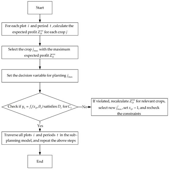
Figure 1.
Flowchart of the greedy algorithm.
According to Figure 1:
- Greedy selection step
For the subsystem-programming model , under the conditions of plot and period , we calculated the expected profit for each type of crop . We then selected the crop that maximized and denoted as the decision to plant . Thus, was formulated as follows:
- 2.
- Examination and adjustment of constraints
After completing greedy selection, it was necessary to examine and adjust the set of constraints in the subsystem model. For , we let denote the decision domain . Specifically, we introduced a constraint violation flag . If (indicating ), we defined as the set of crop types from the original set that caused the constraint violation. That is, when considering the decision-making variables related to , the constraint was not satisfied. Then, we recalculated the relevant for the violated part, re-selected a new from the valid crop set , set , and repeated the constraint check. This process was continued until all were satisfied. Thus, was formulated as follows:
- 3.
- Iterative computation
For the parcel with and period , we repeatedly performed greedy selections and constraint adjustments. Specifically, in each iteration, we first executed the greedy selection step to determine the optimal crop. Then, we checked whether all constraints were satisfied. If violations exist, adjust as per the rules. The above steps were repeated until the entire agricultural planting planning cycle was completed. This process generates an optimal decision set for maximizing agricultural planting profit.
3. Case Study
3.1. Study Area
The study area is located in the mountainous region of North China (Figure 2), characterized by a combination of temperate continental climate and mountain microclimate. The average annual temperature is relatively low, with significant diurnal temperature variations, and precipitation is primarily concentrated in the summer. However, the region enjoys sufficient sunlight throughout the year. The complex topography has fostered a diverse agricultural system: in flat dry lands, sandy loam soil with moderate water and nutrient retention capacity is suitable for drought-resistant crops such as corn and legumes; in terraced fields, the distinct soil layers and high organic matter content make them ideal for root crops such as potatoes; in slope areas, where soil erosion risk is higher, improved plots can support nitrogen-fixing pioneer crops like alfalfa, which also contribute to ecological restoration.
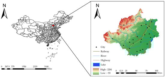
Figure 2.
Overview of the rural geography.
The region is currently undergoing a critical transition from traditional dry farming (primarily wheat-based) to diversified and modern agricultural production models. In open-field cultivation, the ratio of traditional staple crops (e.g., wheat) to cash crops (e.g., broccoli) is dynamically adjusted based on market demand. In facility agriculture, ordinary greenhouses extend the production cycle of spring and autumn vegetables, while intelligent greenhouses enable precise environmental control for the efficient cultivation of off-season vegetables and edible fungi. Since 2023, the region has implemented a three-year legume crop rotation system, prohibiting continuous cropping on all plots (including greenhouses) alongside the promotion of large-scale planting layouts to enhance mechanized operation efficiency.
As a typical representative of agricultural modernization in the mountainous areas of North China, the unique topographic and climatic diversity of this region, combined with the integration of traditional and modern technologies, provide an experimental environment for exploring crop adaptation strategies. This study adopted a decomposition-based stochastic multilevel binary optimization model to reveal planting rules through data-driven methods and formulate adaptation plans to help achieve sustainable agricultural development in similar mountainous areas.
3.2. Data
3.2.1. Data Sources
The data for this study were collected by the research team in collaboration with the local agricultural department in the mountainous area of North China. The main sources included historical records of land use, crop planting structure, and yields provided by the county-level agricultural department, detailed information on land use patterns, crop rotation practices, and greenhouse management obtained through field research in multiple representative villages. For detailed data, please refer to the Supplementary Materials.
3.2.2. Data Description and Data Processing
We focused on collecting data related to rural cultivated land and crops in 2023 (Table 1). Cultivated land covers six types, namely flat dry lands, terraced fields, sloping lands, irrigated lands, ordinary greenhouses, and smart greenhouses. Different types of cultivated land are suitable for corresponding planting modes due to differences in soil characteristics and environmental conditions. At the crop level, there were a total of 41 types, broken down into 16 types of food crop, 21 types of vegetable, and 4 types of edible fungi. According to the planting cycle, there were 16 single-season records and 25 double-season records: single-season crops are mainly distributed in arid land and some irrigated areas, relying on the natural climate to complete single-season growth; double-season crops, on the other hand, achieve annual production through irrigation systems and environmental control technology, thereby improving land utilization.

Table 1.
Basic information on the data of the research area.
Additionally, the 2023 crop planting dataset included detailed information such as sales volume, yield per mu, planting cost, and selling price. For example, in plot A1 (flat dry lands), 80 mu of wheat was planted, with a yield of 800 jin per mu, a planting cost of 450 yuan per mu, and a selling price ranging from CNY 3.00 to 4.00 per jin. These data reflect the economic performance and production characteristics of the local agriculture, providing a solid foundation for subsequent research and decision-making.
In the data preprocessing stage, we implemented a series of measures to address the challenges posed by multisource data and inconsistent formats. First, we conducted data cleaning to eliminate records with abnormal formats, ensuring data integrity. Second, rule-based logic was applied to exclude records missing key information. Finally, a “crop–plot–season” ternary composite label was constructed to accurately capture the dynamic planting patterns. These steps ensured data accuracy and usability.
3.3. Application in Rural Crop Planting Planning
Crop cultivation in rural areas is characterized by many uncertainties, with various interrelated factors influencing the outcomes. These factors include the crop yield per mu, selling prices, expected sales volume, and planting cost. Notably, the crop yield per mu and the selling price of edible fungi followed a uniform distribution. Specifically, the range for crop yield varied between −10% and 10%, and the selling price of edible fungi ranged between −5% and −1%. Additionally, the planting cost, expected sales volume, and vegetable selling prices were projected to increase annually by 5%, while the crop selling prices were projected to remain stable.
Based on the empirical data of the villages in the mountainous areas of North China, the model proposed in this study was divided into four subplanning models in the two dimensions of land resource management and crop planting planning, as follows:
- Subsystem-planning model I: Planting planning model for rice in irrigated lands
Given the unique high water consumption characteristics of rice, whose growth conditions and management modes differ from other crops, we classified rice cultivation on irrigated lands as a subsystem.
We let denote the set of irrigated lands, the set of rice, as the time, and as a very small number. As no constraints were related to restrictions on repeated cropping, crop rotation association constraints, or constraints on planting dispersion for rice cultivation in irrigated lands, we defined and . The model was formulated as follows:
- 2.
- Subsystem-planning model II: Planting planning model for non-rice seasonal food crops in flat dry lands, terraced fields, and sloping lands
Non-rice food crops have strong adaptability to water, can be grown in a wide range of land, and are all single-season crops. Therefore, their cultivation in flat drylands, terraced fields, and sloping lands was classified into a subsystem.
We let denote the collection of flat dry lands, terraced fields, and sloping lands, denote the set of non-rice seasonal food crops, and denote the time set. Let be a very small number. To ensure that the cultivation of non-rice seasonal food crops was not overly dispersed and to adhere to the constraints regarding the threshold area for crop planting on these parcels, we defined , , , and . The model was formulated as follows:
- 3.
- Subsystem-planning model III: Planting planning model for double-crop vegetables in irrigated lands, ordinary greenhouses, and smart greenhouses
Double-cropping vegetables adopt double-cropping planting. Irrigated lands secure water sources, and greenhouses control the basic temperature and humidity. Due to these characteristics, the planting model in water-irrigated lands and greenhouses formed a subsystem.
We let denote the collection of irrigated lands, ordinary greenhouses, and smart greenhouses, the collection of double-crop vegetables, and denotes the time set. To ensure that the planting of double-crop vegetables did not become overly dispersed and to adhere to constraints on the threshold area for crop cultivation within these plots, we defined , , , and . Thus, the model was as follows:
- 4.
- Subsystem-planning model IV: Cultivation planning model for edible fungi in ordinary greenhouses during the second season
Edible fungi demand a stable temperature and humidity. Open-air cultivation may reduce the yield and quality, so greenhouse facilities are needed for precise control. Given its environmental sensitivity, its greenhouse cultivation mode was set as a separate submodel.
Ordinary greenhouses were denoted as , with representing the collection of edible fungi and denoting the time set. When cultivating edible fungi in ordinary greenhouses, there were no constraints related to restrictions on repeated cropping, crop rotation association constraints, or constraint on planting dispersion. We defined and . Thus, the model was as follows:
4. Results
4.1. Analysis of Rural Crop Planting Profits and Planting Plans from 2024 to 2026 Under the Influence of Uncertainty Factors
Under the influence of uncertainties related to expected sales volume, yield per mu, planting cost, and selling prices, we can conclude that the crop planting profits for the village from 2024 to 2026 are projected to be CNY 5.15 × 10⁶, CNY 4.19 × 10⁶, and CNY 5.06 × 10⁶, respectively (Figure 3). Compared with the crop planting profit of CNY 4.89 × 10⁶ in 2023, the total profits for 2024 and 2026 exceeded those of 2023, and the profit for 2025 was less than that of the previous year.
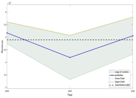
Figure 3.
Trend of crop profits from 2024 to 2026 under the influence of uncertainty.
From 2024 to 2026, multiple constraints (e.g., issues related to crop rotation), the implementation of legume cropping patterns, and limitations on planting dispersion positively influenced the crop growth and development. These factors optimize the growing environment and increase the convenience of field management operations. From the perspective of uncertainty factors, the range between the upper and lower limits remained within reasonable intervals. The sales prices of agricultural products shown an upward trend. Although the planting costs increased, these constraints ensured stability in the planting area and yield, resulting in the total profit levels exceeding those in 2023.
By 2025, repeated cropping restrictions and overly strict legume rotation regulations reduced the planting scheme flexibility. While controlling the planting dispersion reduced the risks, it raised the management costs. Additionally, declining sales prices for edible fungi, coupled with ongoing increases in cultivation expenses, led to suboptimal crop yields that did not meet the expectations. Furthermore, multiple interacting factors expanded the volatility of uncertainties, causing the total profit for 2025 to be lower than that for 2023.
Figure 4 presents the crop planting schemes for specific plots under the influence of uncertainty factors from 2024 to 2026.
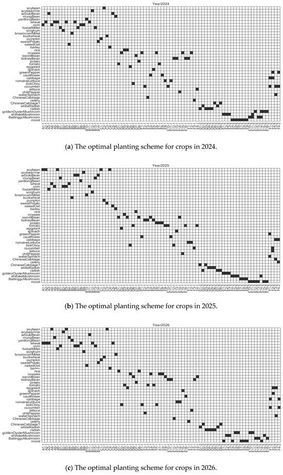
Figure 4.
Optimal planting scheme for crops from 2024 to 2026. Black squares denote planted crops. White squares denote areas that remain unplanted. Horizontal axis denotes plots of land, with −1 and −2 denoting the first and second seasons of cultivation, respectively. Vertical axis indicates the cultivated crop type.
The 2024–2026 crop planting schemes were dynamically adjusted. There were five land types, namely flat dry lands, terraced fields, sloping lands, irrigated lands, and greenhouses, each with their own unique planting plan. Given the existing uncertainties, plots are preferably allocated for high-return crops to improve the profitability.
Furthermore, due to rotation restrictions and the soil fertility maintenance role of leguminous crops, flat dry lands, terraced fields, and sloping lands are primarily cultivated with staple foods such as legumes. Irrigated fields and ordinary and smart greenhouses have focused on the cultivation of vegetables (beans). Based on the constraints related to crop rotation and the requirements for planting diversification across the years, various crop varieties are rotated within each plot. This strategy effectively mitigates problems associated with continuous cropping and facilitates field management practices that ensure optimal growth conditions in suitable soil environments and reasonable planting densities. This approach aims to secure stable long-term agricultural profits.
4.2. Evaluation of Optimization of Planting Models Based on Indicators
To further illustrate the optimization effectiveness of the planting model constructed in this study for practical applications, we introduced two key indicators, the Herfindahl–Hirschman index (HHI) and the rotation frequency of bean crops, for a comprehensive evaluation.
4.2.1. Assessing Crop Planting Concentration via the HHI
The HHI is primarily used to measure the market concentration and is widely applied in antitrust analyses, the formulation of competition policies, and the assessment of corporate mergers [58]. We used the HHI to evaluate the degree of concentration of crop planting distribution across different plots and examined the optimization effects of the planting models.
We let there be a total of plots cultivated with a certain crop. The area of the plot designated for the cultivation of this crop accounted for a proportion of the total cultivated area. The formula for calculating the HHI related to crop cultivation was
In this context, ∈ [0, 1], when is distributed uniformly and the total sum of is relatively small, resulting in an HHI close to zero. This indicates a dispersed crop cultivation pattern. Conversely, if there are significant disparities in , the total sum of increases the HHI, signifying a concentration in crop planting.
Thus, we present the HHI values of five crop categories, namely crops (beans), crops, vegetables (beans), vegetables, and edible fungi, from 2023 to 2026 (Figure 5).
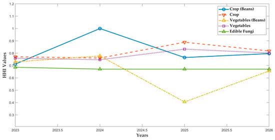
Figure 5.
HHI values of five types of crops from 2023 to 2026.
As shown in Figure 5, the HHI values of the different crop types exhibited distinct variations. Edible fungi were primarily cultivated in ordinary greenhouses during the second season, resulting in a relatively concentrated planting pattern. Thus, their HHI values remained stable. The HHI values for vegetables and crops showed gradual changes, mainly because of the absence of restrictions related to crop rotation and their relative stability when experiencing uncertain factors, leading to minor fluctuations in the planting arrangements. The HHI values for crops (beans) and vegetables (beans) varied significantly. These variations were attributed to multiple uncertainty factors and constraints (e.g., replanting issues, legume crop rotations, and degrees of planting dispersion). These interrelated factors contributed to continuous adjustments in the planting layouts, as reflected in the fluctuating HHI values. Overall, compared with the model’s performance in 2023, the model exhibited improved optimization capabilities when confronted with uncertainty.
4.2.2. Rotation Frequency of Bean Crops
We let denote the total number of plots, and denote the number of plots planted with leguminous crops over a consecutive 3-year period. The formula for calculating the rotation frequency of bean crops was
In this context, when was applied, the planting scheme adhered to the constraints of crop rotation, but when was implemented, certain plots did not comply with the requirements for legume rotation.
Thus, we calculated the crop rotation frequency of leguminous crops for seven types of land (flat dry lands, terraced fields, sloping lands, irrigated lands, ordinary greenhouses, smart greenhouses in the first season, and smart greenhouses in the second season) from 2023 to 2025 and 2024 to 2026. This analysis evaluated the rotation frequency of bean crops using this model (Figure 6).
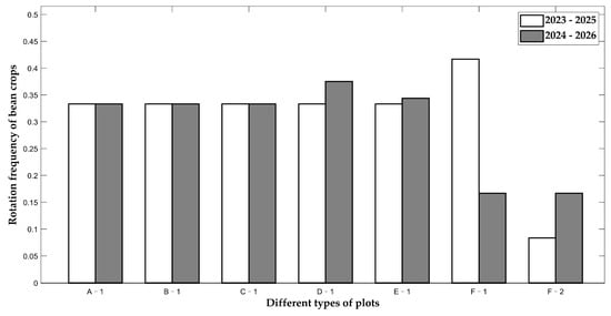
Figure 6.
Rotation frequency of bean crops from 2023 to 2025 and 2024 to 2026.
According to Figure 6, compared with 2023–2025, from 2024 to 2026, the first and second seasons of smart greenhouses had a relatively high and stable crop rotation frequency for leguminous crops. The rotation frequencies for the flat dry lands, terraced fields, sloped areas, irrigated lands, and ordinary greenhouses remained consistent and satisfied the constraints associated with bean crop rotation. These results indicate that the model comprehensively considered various factors across plots and optimized them accordingly. Consequently, these crop rotation frequencies ensured the rationality of crop rotation and maximized the advantages of each type of plot, safeguarding sustainability and efficiency within the entire agricultural system.
5. Sensitivity Analysis
5.1. Parameter Interval Setting
This study used sensitivity analysis to assess the robustness of the model to input parameters and systematically analyzed the mechanism by which five key variables affected the objective function. Based on differences in variable characteristics, these were categorized into two types: endogenous dynamic variables and exogenous benchmark variables. Endogenous dynamic variables included the annual rate of change in crop yield per mu and the annual rate of change in edible fungi selling price . Exogenous benchmark variables encompassed the annual rate of change in planting cost , the annual rate of change in expected sales volume , and the annual rate of change in selling prices (except edible fungi). The robustness of the model to changes in different variables was judged by analyzing the impact of coupled changes in endogenous dynamic variables and external benchmark variables on the model’s output, revealing the model’s response thresholds to rising costs, fluctuating demand, and changes in the prices of conventional agricultural products.
Specifically, we defined the fluctuation ranges and step size for both the endogenous dynamic variables and exogenous baseline variables. Among the endogenous dynamic variables, the annual rate of change in crop yield had a fluctuation range of [−10%, +10%], and the annual rate of change in edible fungus selling price had a fluctuation range of [−5%, −1%], with both undergoing at a 1% step size. Among the exogenous baseline variables, the benchmark values for the annual rate of change in crop planting cost , the annual rate of change in expected crop sales volume , and the annual rate of change in selling price were set to an annual growth rate of +5%. To verify the model’s stability under different conditions, this study uniformly expanded the fluctuation range of these three variables to [−20%, +20%], conducted at a 2% step size.
5.2. Sensitivity Coefficient Calculation Formula
To further investigate the extent to which changes in the parameter combinations affect revenues, this study introduced the bivariate sensitivity coefficient formula and applied it to analyze the revenue scenario. The calculation formula was as follows:
In the formula, represents the return after joint variation, is the initial benchmark return, and denotes the return change amount. and represent the factor variables involved in pairwise joint variation. and are the initial values of these two factor variables, respectively, while and are the change amounts of the factor variables.
Taking the annual change rate of crop planting cost and the annual change rate of expected sales volume as examples, this study elaborated in detail: when the annual change rate of crop planting cost becomes (with a change amount of ) and the expected sales volume becomes (with a change amount of ), the return after joint variation is denoted as . The return change amount is . According to the sensitivity coefficient calculation formula, the calculated at this point is the sensitivity coefficient after the pairwise joint variation of the crop planting cost and expected sales volume: . Similarly, calculating and analyzing the sensitivity coefficients of other variables across different return scenarios enabled a comprehensive and in-depth understanding of the model’s sensitivity to various parameter changes.
5.3. Results of Sensitivity Analysis
5.3.1. Results of Sensitivity Analysis of Endogenous Dynamic Variables
We investigated the impact of the coordinated changes on the endogenous dynamic variables, namely the annual rate of change in crop yield per mu, , and the annual rate of change in the selling price of edible fungi, , on the model’s revenue. A quantitative analysis was used to derive the corresponding sensitivity coefficients, as shown in Figure 7.
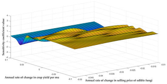
Figure 7.
Sensitivity analysis of the impact of the endogenous dynamic variable coupling on the model. The horizontal axis represents the annual rate of change in selling price of edible fungi, the vertical axis represents the annual rate of change in crop yield per mu, and the z-axis represents the sensitivity coefficient value. The different colors on the surface plot are used to represent the differences in the sensitivity coefficient value.
As can be seen from Figure 7, the model demonstrated good stability whether the sales price of edible fungi or the crop yield per mu changed or not. When the annual rate of change in crop yield per mu remained stable and the annual rate of change in the sales price of edible fungi fluctuated within the common range of −0.05 to −0.01, the sensitivity coefficient changed within a small range. Even when the price change rate approached the boundary value, the fluctuation of the model’s sensitivity coefficient still remained within an acceptable range, demonstrating strong robustness. Similarly, when the annual rate of change in the selling price of edible fungi remained stable and the annual rate of change in crop yield per mu varied within the normal production fluctuation range of −0.1 to 0.1, the sensitivity coefficient also maintained good stability.
Admittedly, there were local areas in the graph where the sensitivity coefficients fluctuated greatly. However, these areas accounted for a small proportion and represented low-probability scenarios. In contrast, the model’s stability in most areas was the primary feature, indicating that the model can reliably reflect the relationship between revenue and variables in most actual situations, providing decision-makers with a stable and valuable reference.
5.3.2. Results of Sensitivity Analysis of Exogenous Benchmark Variables
For the exogenous benchmark variables, including the annual rate of change in expected crop sales volume , the annual rate of change in crop planting cost , and the annual rate of change in selling price of crops (except edible fungi) , the study analyzed the impact of their coordinated changes on the model’s revenue and calculated the corresponding sensitivity coefficients, as shown in Figure 8.
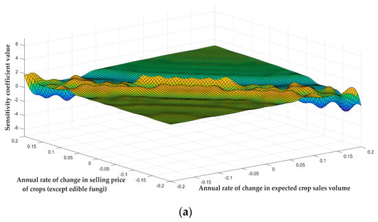
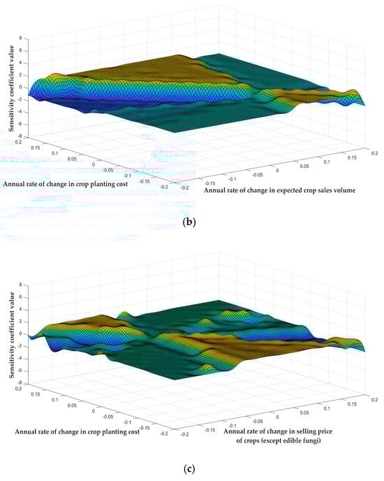
Figure 8.
Sensitivity analysis of the impact of exogenous benchmark variable coupling on the model. The horizontal and vertical axes in the figures represent the annual rates of change of different parameters, and the vertical axis represents the sensitivity coefficient value. (a) Sensitivity coefficients under the coupling of changes in expected crop sales volume and selling price of crops (except edible fungi). (b) Sensitivity coefficients under the coupling of changes in crop planting cost and expected crop sales volume. (c) Sensitivity coefficients under the coupling of changes in crop planting cost and selling price of crops (except edible fungi). The different colors on the surface plot are used to represent the differences in the sensitivity coefficient value.
Figure 8a–c shows the dynamic coupling relationships between three groups of exogenous benchmark variables: the annual rate of change in the expected crop sale volume and selling price, the annual rate of change in planting cost and expected crop sale volume, and the annual rate of change in the planting cost and selling price. A comparative analysis showed that these three graphs shared a significant common feature: within the range of variation of most parameters, the sensitivity coefficients of the model maintained a relatively stable fluctuation state. This phenomenon shows that the model has good robustness to coordinated changes in parameters within the normal range, and that the model’s income will not fluctuate violently due to normal market parameter fluctuations.
Although there were local areas of sensitivity coefficient fluctuations in all three graphs, these fluctuations only occurred within a limited range of parameters and accounted for a small proportion. In terms of differences, there were slight differences in the degree and scope of the impact of parameter fluctuations on the sensitivity coefficient in different graphs, but these differences did not change the overall stability of the model.
The comprehensive research results show that when two exogenous benchmark variables change in a coordinated manner, the model can maintain a stable response in the vast majority of cases. Although changes in the sensitivity coefficients may occur in certain parameter intervals, these local fluctuations do not affect the robustness of the model in the overall parameter range.
6. Discussion
6.1. Establishment of Benchmark Models
When verifying the performance of a model, it is common to establish a benchmark model to compare and determine whether it is superior to other models. This approach has been applied in many optimization problems [59,60]. However, in the field of agricultural optimization models, there is currently no universal benchmark model. The model constructed in this paper organically combines land constraints with market uncertainty. In order to evaluate this model, we established two benchmark models based on this model by removing the land constraint module and the market uncertainty module, respectively, and then compared and analyzed them with the model in this paper. The specific definitions are as follows.
- Pure land constraint model
This category focused exclusively on land “hardware” factors such as land suitability, crop rotation feasibility, and planting dispersion regulations during agricultural planning while neglecting dynamic market uncertainties. For instance, Thilagavathi et al. [44] emphasized land physical characteristics and related constraints, employing a social spider algorithm (SSA) to optimize crop planting areas and productivity. This provided a profit-oriented direction for agricultural planning. However, by excluding market price fluctuations and demand variations, this model risks missing market opportunities during macro-level land allocation strategy formulation, thereby limiting the economic potential of land resources.
- 2.
- Pure uncertainty model
This category prioritized market uncertainties like price volatility and yield variability while completely disregarding the land’s natural attributes and physical limitations. Ahumada et al. [45], for example, developed a two-stage stochastic programming model to optimize fresh agricultural product production in response to demand uncertainty. This approach relies solely on market trends and yield projections when formulating land strategies, without accounting for constraints such as land carrying capacity, crop rotation requirements, and planting dispersion. By assuming infinite land resource availability, this model may generate unrealistic allocation plans.
6.2. Comparison Result
Based on the two benchmark models constructed, we systematically evaluated the differences in the performance of the three models under different revenue scenarios (low, medium, and high) from 2024 to 2026, as shown in Figure 9. In the comparison, our research model is represented as Model A, the baseline model that only considered land constraints is represented as Model B, and the baseline model that only considered uncertainty is represented as Model C.
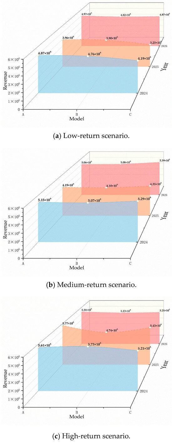
Figure 9.
Benefit performance of the three models in different years and income scenarios.
In the low-return scenario (Figure 9a), Model A’s returns in 2024 (CNY 4.87 × 10⁶) and 2026 (CNY 4.97 × 10⁶) exceeded those of Models B and C. Though its 2025 return (CNY 3.96 × 10⁶) declined, the drop was smaller than that of Model B (CNY 3.90 × 10⁶) and Model C (CNY 3.25 × 10⁶). This highlights Model A’s risk resistance: by accounting for both land constraints and uncertainty, it maintained relatively stable returns even in low-return environments. Model B, focusing solely on land constraints, lacked adaptability under uncertainty; and Model C, prioritizing uncertainty factors, ignored the land constraints, leading to volatile returns (e.g., a sharp 2025 decline). Both exemplify the limitations of single-factor models.
In the medium-return scenario (Figure 9b), Model A performed strongly in 2024 (CNY 5.15 × 10⁶) and 2026 (CNY 5.06 × 10⁶), with minimal three-year fluctuation. Model B showed promise in 2024 (CNY 5.07 × 10⁶) and 2026 (CNY 5.08 × 10⁶), but its 2025 return (CNY 4.10 × 10⁶) lagged behind A. Model C had the highest 2024 return (CNY 5.29 × 10⁶) but fluctuated drastically in 2025 (CNY 4.35 × 10⁶) and 2026 (CNY 5.39 × 10⁶). Model A’s strength lay in balancing returns across years via comprehensive constraint optimization, unlike Model B and Model C, which, hindered by single factors, failed to ensure stability in multiperiod returns.
In the high-return scenario (Figure 9c), Model A led in 2024 (CNY 5.61 × 10⁶) and 2025 (CNY 5.77 × 10⁶). While slightly lower than Model B in 2026 (CNY 5.13 × 10⁶), Model A’s three-year returns were more balanced. Model B peaked in 2024 (CNY 5.73 × 10⁶) but dropped sharply in 2025 (CNY 4.74 × 10⁶); Model C’s 2025 return (CNY 5.43 × 10⁶) was outstanding but declined notably in 2026 (CNY 5.21 × 10⁶). Model A’s superiority stemmed from its ability to capture high-return opportunities while mitigating extreme fluctuations through multifactor constraints. In contrast, Model B and Model C relied on single conditions, resulting in volatile returns and poor sustainability.
In summary, Model A achieved a balance between risk and return by incorporating both land constraints and uncertainty factors, and it showed greater stability and comprehensive adaptability in the low-, average-, and high-return scenarios. In contrast, Model B and Model C only considered a single factor, and in the face of environmental changes, their returns fluctuated greatly, exposing the limitations of the strategy.
7. Conclusions
In the study of crop planting planning, we focused on specific land and uncertainty constraints and constructed a decomposition-based stochastic multilevel binary optimization model. The model aims to maximize agricultural profits by taking into account the uncertainties in sales volume, selling price, yield per mu, and planting cost. In addition, we established six types of constraints, including thresholds for the crop area planted per plot, restrictions on repeated cropping, associations with crop rotation, degree of planting dispersion, management of the threshold for the crop area within plots, and the range of variation of uncertain variables, to ensure the comprehensiveness and practicality of the model.
Faced with the complexity of the planting planning problem, we adopted a divide-and-conquer approach, decomposing the problem from the perspectives of crops and plots, and transforming it into multiple manageable subproblems. In this way, we reduced the difficulty and complexity of solving the problem. Subsequently, we used a greedy algorithm to gradually solve these subproblems, which further improved the model solving process.
To verify the effectiveness of the model, we conducted an empirical study with a rural village in the mountainous area of North China as an example, predicted the village’s total agricultural revenue for the three years from 2024 to 2026, and formulated specific crop planting plans for different plots. To evaluate the optimization performance of the model, we used the Herfindahl–Hirschman Index (HHI) and the frequency of legume crop rotation indicators. The results show that from 2024 to 2026, the planting dispersion and rotation frequency of legume crops improved significantly compared with those in 2023. In addition, we conducted a sensitivity analysis, dividing the uncertain variables into endogenous dynamic variables and exogenous benchmark variables, and observed the impact of their coordinated changes on the model’s benefits. In particular, the model output showed good stability when the endogenous dynamic variables (such as the annual rate of change in yield per mu and the selling price of edible fungi) and exogenous benchmark variables (such as planting cost, selling prices, and expected sales volumes) changed.
In order to fully verify the superiority of the proposed model, we set up two benchmark models for comparative analysis: benchmark model 1 only considered the land resource constraints, and benchmark model 2 only considered the uncertainty factors. Through comparative experiments in different years and multiple income scenarios, the results showed that the performance of our model was significantly better than these two benchmark models. This comparison not only verified the effectiveness of the model, but also highlighted the combined advantages of considering both the land constraints and uncertainty factors.
Although the model performed well in both theoretical and empirical studies, it still had some limitations. First, we used a greedy algorithm in the solution process. Although this method can efficiently find a local optimal solution, it may not guarantee a global optimal solution. This means that in some cases, the optimization results of the model may not be the most ideal planting plan. Second, the model’s assumptions about uncertainty may not fully reflect the complexity and dynamic changes in reality. For example, extreme weather events (such as droughts and floods) or sudden market fluctuations (such as price crashes or supply chain disruptions) can have a significant impact on agricultural production.
In summary, our model provides a reference for crop planting planning by comprehensively considering the land constraints and uncertainty factors. It aims to help agricultural managers optimize resource allocation and promote sustainable agricultural development. In order to further improve the practicality and stability of the model, future research should focus on optimizing the model in complex and uncertain environments, incorporate more uncertainty factors, and further improve the algorithm to overcome the limitations of the greedy algorithm to better support agricultural production practices.
Supplementary Materials
The following supporting information can be downloaded at: www.mdpi.com/article/10.3390/math13071213/s1. The data for this study were collected by the research team in collaboration with the local agricultural department in the mountainous area of North China. Detailed data, please refer to the supplementary materials.
Author Contributions
Conceptualization, F.W., Y.L., W.Z. and Y.Y.; Methodology, F.W., Y.L., W.Z. and Y.Y.; Software, W.Z. and Y.Y.; Validation, F.W. and W.Z.; Formal analysis, F.W.; Data curation, F.W. and W.Z.; Writing—original draft, F.W.; Writing—review and editing, F.W. and Y.L.; Visualization, F.W.; Supervision, F.W. and Y.L.; Funding acquisition Y.L. All authors have read and agreed to the published version of the manuscript.
Funding
This research was funded by the National Natural Science Foundation of China (grant number 11701161) and the National Social Sciences Foundation of China (24BTJ068).
Data Availability Statement
All experimental data can be obtained by contacting the corresponding author.
Acknowledgments
We greatly appreciate the efforts made by the reviewers and editorial team for our article.
Conflicts of Interest
The authors declare no conflicts of interest.
Abbreviation
The following abbreviation was used in this manuscript:
| HHI | Herfindahl–Hirschman index |
References
- Hodge, I. Uncertainty, irreversibility and the loss of agricultural land. J. Agric. Econ. 1984, 35, 191–202. [Google Scholar]
- Chen, Q.; Xie, H. Temporal-spatial differentiation and optimization analysis of cultivated land green utilization efficiency in China. Land 2019, 8, 158. [Google Scholar] [CrossRef]
- Wang, J.; Li, Y.; Wang, Q.; Cheong, K.C. Urban–rural construction land replacement for more sustainable land use and regional development in China: Policies and practices. Land 2019, 8, 171. [Google Scholar] [CrossRef]
- Hufnagel, J.; Reckling, M.; Ewert, F. Diverse approaches to crop diversification in agricultural research. A review. Agron. Sustain. Dev. 2020, 40, 14. [Google Scholar]
- Liu, Z.; Yang, P.; Wu, W.; You, L. Spatiotemporal changes of cropping structure in China during 1980–2011. J. Geogr. Sci. 2018, 28, 1659–1671. [Google Scholar]
- Ozsahin, E.; Sari, H.; Ozdes, M.; Eroglu, I.; Yuksel, O. Determination of suitable lands for rice cultivation in Edirne plain: GIS supported FAO limitation method. Paddy Water Environ. 2022, 20, 325–338. [Google Scholar]
- Song, G.; Zhang, H. Cultivated land use layout adjustment based on crop planting suitability: A case study of typical counties in Northeast China. Land 2021, 10, 107. [Google Scholar] [CrossRef]
- Zhang, B.; Wu, Y.; Zhao, B.; Chanussot, J.; Hong, D.; Yao, J.; Gao, L. Progress and challenges in intelligent remote sensing satellite systems. IEEE J. Sel. Top. Appl. Earth Observ. Remote Sens. 2022, 15, 1814–1822. [Google Scholar] [CrossRef]
- Huang, Q.; Tang, H.; Zhou, Q.; Wu, W.; Wang, L.; Zhang, L. Remote-sensing based monitoring of planting structure and growth condition of major crops in Northeast China. Trans. Chin. Soc. Agric. Eng. 2010, 26, 218–223. [Google Scholar]
- Wang, H.; Pan, X.; Luo, J.; Luo, Z.; Chang, C.; Shen, Y. Using remote sensing to analyze spatiotemporal variations in crop planting in the North China Plain. Chin. J. Eco-Agric. 2015, 23, 1199–1209. [Google Scholar]
- Rabia, A.H.; Neupane, J.; Lin, Z.; Lewis, K.; Cao, G.; Guo, W. Principles and applications of topography in precision agriculture. Adv. Agron. 2022, 171, 143–189. [Google Scholar]
- Villa, G.; Adenso-Díaz, B.; Lozano, S. An analysis of geographic and product diversification in crop planning strategy. Agric. Syst. 2019, 174, 117–124. [Google Scholar] [CrossRef]
- Benini, M.; Blasi, E.; Detti, P.; Fosci, L. Solving crop planning and rotation problems in a sustainable agriculture perspective. Comput. Oper. Res. 2023, 159, 106316. [Google Scholar] [CrossRef]
- Almagro, M.; Re, P.; Díaz-Pereira, E.; Boix-Fayos, C.; Sánchez-Navarro, V.; Zornoza, R.; Martínez-Mena, M. Crop diversification effects on soil organic carbon and nitrogen storage and stabilization is mediated by soil management practices in semiarid woody crops. Soil Tillage Res. 2023, 233, 105815. [Google Scholar] [CrossRef]
- Thilakarathne, N.N.; Bakar, M.S.A.; Abas, P.E.; Yassin, H. Towards making the fields talks: A real-time cloud enabled IoT crop management platform for smart agriculture. Front. Plant Sci. 2023, 13, 1030168. [Google Scholar] [CrossRef]
- Kar, G.; Chaudhari, S.K.; Patra, P.K.; Dixit, P.R.; Alam, N.M. GIS based sustainable land use planning using spatial variation of soil and terrain information. J. Agric. Phys. 2020, 20, 15–21. [Google Scholar]
- Borah, N.; Ladon, P.; Garkoti, S.C. Ethnopedological knowledge of upland Karbi Community: A case study from Dima Hasao District of Assam, North-Eastern Himalaya, India. Indian J. Tradit. Knowl. 2023, 22, 30–39. [Google Scholar]
- Saleem, M.; Pervaiz, Z.H.; Contreras, J.; Lindenberger, J.H.; Hupp, B.M.; Chen, D.; Zhang, Q.; Wang, C.; Iqbal, J.; Twigg, P. Cover crop diversity improves multiple soil properties via altering root architectural traits. Rhizosphere 2020, 16, 100248. [Google Scholar] [CrossRef]
- Gutknecht, J.; Journey, A.; Peterson, H.; Blair, H.; Cates, A. Cover crop management practices to promote soil health and climate adaptation: Grappling with varied success from farmer and researcher observations. J. Environ. Qual. 2023, 52, 448–464. [Google Scholar] [CrossRef]
- Yang, L.; Chen, Y.; Ma, X.; Qiu, Q.; Peng, R. A prognosis-centered intelligent maintenance optimization framework under uncertain failure threshold. IEEE Trans. Reliab. 2023, 73, 115–130. [Google Scholar] [CrossRef]
- Chen, L.; Dong, T.; Peng, J.; Ralescu, D. Uncertainty analysis and optimization modeling with application to supply chain management: A systematic review. Mathematics 2023, 11, 2530. [Google Scholar] [CrossRef]
- Han, S.; Li, H.; Li, M.; Zhang, J.; Guo, R.; Ma, J.; Zhao, W. Deep learning–based stochastic modelling and uncertainty analysis of fault networks. Bull. Eng. Geol. Environ. 2022, 81, 242. [Google Scholar]
- Muñoz, D.F.; Moftakhari, H.; Moradkhani, H. Quantifying cascading uncertainty in compound flood modeling with linked process-based and machine learning models. Hydrol. Earth Syst. Sci. 2024, 28, 2531–2553. [Google Scholar] [CrossRef]
- Alemany, M.M.E.; Esteso, A.; Ortiz, Á.; del Pino, M. Centralized and distributed optimization models for the multi-farmer crop planning problem under uncertainty: Application to a fresh tomato Argentinean supply chain case study. Comput. Ind. Eng. 2021, 153, 107048. [Google Scholar]
- Borah, G.; Dutta, P. Fuzzy risk analysis in crop selection using information measures on quadripartitioned single-valued neutrosophic sets. Expert Syst. Appl. 2024, 255, 124750. [Google Scholar] [CrossRef]
- Liu, F.; Li, W.; Wang, X.; Zhang, Y.; Ding, Z.; Xu, Y. Water–Food Nexus System Management under Uncertainty through an Inexact Fuzzy Chance Constraint Programming Method. Water 2024, 16, 227. [Google Scholar] [CrossRef]
- Jayne, T.S. Do high food marketing costs constrain cash crop production? evidence from Zimbabwe. Econ. Dev. Cult Change 1994, 42, 387–402. [Google Scholar] [CrossRef][Green Version]
- Fafchamps, M. Cash crop production, food price volatility, and rural market integration in the third world. Am. J. Agric. Econ. 1992, 74, 90–99. [Google Scholar]
- Narayanamoorthy, A. Profitability in crops cultivation in India: Some evidence from cost of cultivation survey data. Indian J. Agric. Econ. 2013, 68, 104–121. [Google Scholar]
- Mani, V.S.; Gautam, K.C.; Chakraborty, T.K. Losses in crop yield in India due to weed growth. Int. J. Pest Manag. C 1968, 14, 142–158. [Google Scholar]
- Guo, S.; Zhang, F.; Engel, B.A.; Wang, Y.; Guo, P.; Li, Y. A distributed robust optimization model based on water-food-energy nexus for irrigated agricultural sustainable development. J. Hydrol. 2022, 606, 127394. [Google Scholar] [CrossRef]
- Guo, S.; Guo, P. A two-stage joint chance-constrained programming considering compound uncertainty of interval, random and fuzzy: A case study for agricultural water planning in an arid area. Stoch. Environ. Res. Risk Assess. 2022, 36, 3281–3293. [Google Scholar] [CrossRef]
- Cao, K.; Batty, M.; Huang, B.; Liu, Y.; Yu, L.; Chen, J. Spatial multi-objective land use optimization: Extensions to the non-dominated sorting genetic algorithm-II. Int. J. Geogr. Inf. Sci. 2011, 25, 1949–1969. [Google Scholar] [CrossRef]
- Stewart, T.J.; Janssen, R.; Van Herwijnen, M. A genetic algorithm approach to multiobjective land use planning. Comput. Oper. Res. 2004, 31, 2293–2313. [Google Scholar] [CrossRef]
- Duh, J.D.; Brown, D.G. Knowledge-informed Pareto simulated annealing for multi-objective spatial allocation. Comput. Environ. Urban Syst. 2007, 31, 253–281. [Google Scholar] [CrossRef]
- Santé-Riveira, I.; Boullón-Magán, M.; Crecente-Maseda, R.; Miranda-Barrós, D. Algorithm based on simulated annealing for land-use allocation. Comput. Geosci. 2008, 34, 259–268. [Google Scholar] [CrossRef]
- Liu, X.; Ou, J.; Li, X.; Ai, B. Combining system dynamics and hybrid particle swarm optimization for land use allocation. Ecol. Model. 2013, 257, 11–24. [Google Scholar] [CrossRef]
- Masoomi, Z.; Mesgari, M.S.; Hamrah, M. Allocation of urban land uses by Multi-Objective Particle Swarm Optimization algorithm. Int. J. Geogr. Inf. Sci. 2013, 27, 542–566. [Google Scholar] [CrossRef]
- Yu, J.; Chen, Y.; Wu, J. Modeling and implementation of classification rule discovery by ant colony optimisation for spatial land-use suitability assessment. Comput. Environ. Urban Syst. 2011, 35, 308–319. [Google Scholar] [CrossRef]
- Mousa, A.A.; El-Desoky, I.M. Stability of Pareto optimal allocation of land reclamation by multistage decision-based multipheromone ant colony optimization. Swarm Evol. Comput. 2013, 13, 13–21. [Google Scholar] [CrossRef]
- Wu, L.; Tian, J.; Liu, Y.; Jiang, Z. Multi-objective crop planting structure optimization based on game theory. Water 2022, 14, 2125. [Google Scholar]
- Liu, L.C.; Lv, K.C.; Zheng, Y.J. Crop cultivation planning with fuzzy estimation using water wave optimization. Front. Plant Sci. 2023, 14, 1139094. [Google Scholar] [CrossRef] [PubMed]
- Zheng, Y.J.; Ling, H.F. Emergency transportation planning in disaster relief supply chain management: A cooperative fuzzy optimization approach. Soft Comput. 2013, 17, 1301–1314. [Google Scholar]
- Thilagavathi, N.; Amudha, T. A novel methodology for optimal land allocation for agricultural crops using Social Spider Algorithm. PeerJ 2019, 7, e7559. [Google Scholar] [CrossRef]
- Ahumada, O.; Villalobos, J.R.; Mason, A.N. Tactical planning of the production and distribution of fresh agricultural products under uncertainty. Agric. Syst. 2012, 112, 17–26. [Google Scholar]
- Hu, F.; Wang, G. Knowledge reduction based on divide and conquer method in rough set theory. Math. Probl. Eng. 2012, 2012, 864652. [Google Scholar]
- Zhang, Y.; Mei, Y.; Zhang, B.; Jiang, K. Divide-and-conquer large scale capacitated arc routing problems with route cutting off decomposition. Inf. Sci. 2021, 553, 208–224. [Google Scholar]
- Ren, Z.; Chen, A.; Wang, M.; Yang, Y.; Liang, Y.; Shang, K. Bi-hierarchical cooperative coevolution for large scale global optimization. IEEE Access 2020, 8, 41913–41928. [Google Scholar]
- Ji, R.; Zhao, Y.; Xiong, Y.; Wang, D.; Zhang, L.; Hu, Z. Decomposition-based synthesis for applying divide-and-conquer-like algorithmic paradigms. ACM Trans. Program. Lang. Syst. 2024, 46, 1–59. [Google Scholar]
- Wang, Y. Review on greedy algorithm. Theor. Nat. Sci. 2023, 14, 233–239. [Google Scholar] [CrossRef]
- Xiang, D.; Lin, H.; Ouyang, J.; Huang, D. Combined improved A* and greedy algorithm for path planning of multi-objective mobile robot. Sci. Rep. 2022, 12, 13273. [Google Scholar] [CrossRef]
- Aslan, S. Back-and-Forth (BaF): A new greedy algorithm for geometric path planning of unmanned aerial vehicles. Computing 2024, 106, 2811–2849. [Google Scholar]
- Shen, C.; Ninh, A. Finding the Modes of Some Multivariate Discrete Probability Distributions: Application of the Resource Allocation Problem. Stat. Probab. Lett. 2020, 156, 108579. [Google Scholar] [CrossRef]
- Luo, S.; Wang, Y.; Tang, J.; Guan, X.; Xu, M. Two-Echelon Multidepot Logistics Network Design with Resource Sharing. J. Adv. Transp. 2021, 2021, 6619539. [Google Scholar]
- Liu, S.; Hu, S.; Du, J.; Cao, H.; Zhang, B.; Jiang, Y.; Feng, S. Space Debris Sky Survey Observation Strategy Based on HEALPix and Greedy Algorithm. Aerospace 2025, 12, 168. [Google Scholar] [CrossRef]
- Basile, M.; Nardini, G.; Perazzo, P.; Dini, G. PROACTION: Profitable Transactions Selection Greedy Algorithm in Rational Proof-of-Work Mining. Blockchains 2025, 3, 2. [Google Scholar] [CrossRef]
- Švarcmajer, M.; Ivanović, D.; Rudec, T.; Lukić, I. Application of Graph Theory and Variants of Greedy Graph Coloring Algorithms for Optimization of Distributed Peer-to-Peer Blockchain Networks. Technologies 2025, 13, 33. [Google Scholar] [CrossRef]
- Pavic, I.; Galetic, F.; Piplica, D. Similarities and Differences between the CR and HHI as an Indicator of Market Concentration and Market Power. Br. J. Econ. Manag. Trade 2016, 13, 1–8. [Google Scholar] [CrossRef]
- van Der Meer, D. A benchmark for multivariate probabilistic solar irradiance forecasts. Sol. Energy 2021, 225, 286–296. [Google Scholar] [CrossRef]
- Luan, F.; Zhang, W.; Liu, Y. Robust International Portfolio Optimization with Worst-Case Mean-LPM. Math. Probl. Eng. 2022, 2022, 5072487. [Google Scholar]


Disclaimer/Publisher’s Note: The statements, opinions and data contained in all publications are solely those of the individual author(s) and contributor(s) and not of MDPI and/or the editor(s). MDPI and/or the editor(s) disclaim responsibility for any injury to people or property resulting from any ideas, methods, instructions or products referred to in the content. |
© 2025 by the authors. Licensee MDPI, Basel, Switzerland. This article is an open access article distributed under the terms and conditions of the Creative Commons Attribution (CC BY) license (https://creativecommons.org/licenses/by/4.0/).