Article

Multistage Threshold Segmentation Method Based on Improved Electric Eel Foraging Optimization

College of Computer and Control Engineering, Northeast Foresty University, 26 Hexing Road, Harbin 15004, China
*
Author to whom correspondence should be addressed.
Mathematics 2025, 13(7), 1212; https://doi.org/10.3390/math13071212
Submission received: 31 January 2025 / Revised: 3 March 2025 / Accepted: 25 March 2025 / Published: 7 April 2025

Abstract

:
Multi-threshold segmentation of color images is a critical component of modern image processing. However, as the number of thresholds increases, traditional multi-threshold image segmentation methods face challenges such as low accuracy and slow convergence speed. To optimize threshold selection in color image segmentation, this paper proposes a multi-strategy improved Electric Eel Foraging Optimization (MIEEFO). The proposed algorithm integrates Differential Evolution and Quasi-Opposition-Based Learning strategies into the Electric Eel Foraging Optimization, enhancing its search capability, accelerating convergence, and preventing the population from falling into local optima. To further boost the algorithm’s search performance, a Cauchy mutation strategy is applied to mutate the best individual, improving convergence speed. To evaluate the segmentation performance of the proposed MIEEFO, 15 benchmark functions are used, and comparisons are made with seven other algorithms. Experimental results show that the MIEEFO algorithm outperforms other algorithms in at least 75% of cases and exhibits similar performance in up to 25% of cases. To further explore its application potential, a multi-level Kapur entropy-based MIEEFO threshold segmentation method is proposed and applied to different types of benchmark images and forest fire images. Experimental results indicate that the improved MIEEFO achieves higher segmentation quality and more accurate thresholds, providing a more effective method for color image segmentation.

1. Introduction

With the development of computer computing resources, the field of computer vision has developed rapidly. Image segmentation is not only an important branch of computer vision, but also one of the most difficult problems in image processing [1]. Image segmentation is widely used in automatic driving [2,3], intelligent medicine [4], industrial testing [5] and other fields. Currently, the most widely used image segmentation methods include threshold segmentation [6], edge segmentation [7], region segmentation [8], clustering segmentation [9,10] and deep learning segmentation [11,12]. Threshold segmentation has gained attention due to its simplicity, low computational cost, and ease of implementation. Threshold segmentation has become a research hotspot owing to its advantages of simplicity, small computation and easy solution [13].
Threshold segmentation can be divided into two types, single-threshold segmentation and multi-threshold segmentation [14]. Single-threshold segmentation divides an image into target and background, whereas multi-threshold segmentation segments an image into multiple regions. Because single-threshold segmentation often fails to provide the necessary patterns for the problem at hand, multi-threshold segmentation is generally preferred. However, with the increase in thresholds, the computational complexity of traditional segmentation methods grows exponentially, leading to issues such as low accuracy and slow convergence speed. In order to solve this problem, an increasing number of researchers are introducing swarm intelligence optimization algorithms for image segmentation to enhance accuracy and speed [15]. Common multi-threshold segmentation methods include Otsu’s entropy [16,17], Kapur entropy [18,19], fuzzy entropy [20] and the cross-entropy method [21,22]. The Kapur entropy technique is insensitive to regions and preserves details better, which is why it has been widely applied in multi-level image segmentation.
However, multi-level threshold segmentation techniques rely heavily on threshold combinations and involve a large search space [23]. Therefore, improving the segmentation performance necessitates optimization of the multi-level threshold selection process. Traditional methods often optimize the optimal thresholds by employing operational research techniques or exhaustive enumeration methods. However, as the number of thresholds increases, the computational complexity grows exponentially. To address this issue, researchers have introduced heuristic algorithms, which alleviate the problem of low computational efficiency to a certain extent. Houssein, E. H. et al. [24] proposed an improved chimp optimization algorithm (ICHOA) and applied it to the problem of multi-level threshold image segmentation. Sabha, M. et al. [25] introduced a cooperative simulated meta-heuristic algorithm called CPGH, which combines particle swarm optimization (PSO), gray wolf optimization (GWO), and Harris hawks optimization (HHO)to run in parallel, ultimately applied to coronavirus image segmentation. Hao, S. et al. [26] developed an improved salp swarm algorithm (ILSSA) that integrates chaotic mapping with local escape operators and applied it to dermoscopic skin cancer image segmentation. Chauhan, D. et al. [27] presented a crossover optimization artificial electric field algorithm (AEFA) that uses a Kapur’s entropy function, applied to the Berkeley segmentation dataset. Qian, Y. et al. [28] proposed a continuous foraging ant colony optimization algorithm (SSACO) based on salp foraging (SSACO), and applied it to remote sensing image segmentation. Dhal, K. G. et al. [29] introduced an improved slime mould algorithm (ISMA), employing oppositional learning and differential evolution mutation strategies to enhance the algorithm’s performance, applied to the segmentation of unlabeled white blood cell images. Shi, J. et al. [30] proposed an improved variant of the whale optimization algorithm (GTMWOA) and applied it to lupus nephritis images. Houssein, E. et al. [31] introduced an efficient search rescue optimization algorithm (SAR) based on oppositional learning for segmenting blood cell images and addressing multi-level threshold issues.
SIO is a powerful family of heuristic algorithms that have demonstrated remarkable capabilities in solving computationally intensive and complex problems, where classical algorithms often prove inefficient [32]. In most cases, swarm intelligence algorithms begin by randomly generating a population in the early stages of iteration and utilize specific formulas to explore the search space during the process, ultimately identifying the optimal solution. These operations are inspired by natural phenomena such as natural behaviors, physical rules, social interactions, and evolutionary principles. Representative SIO methods, including Particle Swarm Optimization (PSO) [33], Differential Evolution (DE) [34], Artificial Bee Colony (ABC) [35] and the Whale Optimization Algorithm (WOA) [36], have been successfully applied to various fields such as path planning, power systems and image processing. Although SIO methods differ in form, their core idea remains similar: simulating natural behaviors to construct mathematical models for solving specific problems.
EEFO, a novel SIO algorithm proposed in 2024, simulates the predatory behavior of electric eels [37]. It has been tested using various benchmark functions and engineering problems and compared with standard algorithms such as the Whale Optimization Algorithm (WOA), the Arithmetic Optimization Algorithm (AOA) [38], Harris Hawks Optimization (HHO) [39] and Beluga Whale Optimization (BWO) [40]. Experimental results indicate that EEFO exhibits significant potential. Thus, EEFO holds promise for further research and applications. However, there is still considerable room for improvement when applying EEFO to complex problems such as image segmentation. According to the “No Free Lunch” theorem [41], no algorithm is universally optimal for solving all problems. In other words, every algorithm has its limitations. Nevertheless, its performance can be enhanced by introducing new strategies and adjusting the parameter settings.
In this study, we further develop the EEFO method to enhance its effectiveness in addressing the challenges of color image segmentation.
The main contributions of this study are as follows:
i. This paper proposes an improved Electric Eel Foraging Optimization, which incorporates a differential evolution strategy, a quasi-oppositional learning strategy and the Cauchy mutation strategy, named MIEEFO.
ii. A set of 15 benchmark test functions are used to evaluate the algorithm, and MIEEFO is compared with several state-of-the-art heuristic algorithms. Analysis using different evaluation methods demonstrates that MIEEFO exhibits superior performance.
iii. We introduce an efficient MIEEFO-based color image segmentation technique. Experiments were conducted comparing MIEEFO with other similar algorithms at multiple threshold levels, using Kapur’s entropy as the fitness function. The results show that the segmentation method based on MIEEFO significantly improves the accuracy of image segmentation.
iv. The proposed image segmentation method was applied to forest fire images, providing an effective solution for segmenting forest fire imagery.
The remainder of this paper is organized as follows: Section 2 provides an overview of the EEFO algorithm. Section 3 describes the proposed enhanced MIEEFO algorithm. Section 4 presents the simulation results of MIEEFO for the test functions. Section 5 outlines the image segmentation principles of MIEEFO and provides experimental results of the segmentation method. Finally, Section 6 presents our conclusions and future work.

2. Electric Eel Foraging Optimization

Electric Eel Foraging Optimization (EEFO) [37] was proposed by Weiguo Zhao and Liying Wang et al. in 2024, which simulates the predation behavior of electric eels in nature. The algorithm can be divided into an interacting stage, resting stage, hunting stage and migrating stage. These mechanisms are illustrated in Figure 1.

2.1. Interacting Stage

When eels encounter a school of fish, they interact by swimming and agitating each other. The eels then begin to swim in a large electrified circle, catching many small fish in the center of the circle. The following model represents this churn.
v i ( t + 1 ) = x j ( t ) + C × x ¯ ( t ) x i ( t ) p 1 > 0.5 v i ( t + 1 ) = x j ( t ) + C × x r ( t ) x i ( t ) p 1 0.5 fit x j ( t ) < fit x i ( t ) v i ( t + 1 ) = x i ( t ) + C × x ¯ ( t ) x j ( t ) p 2 > 0.5 v i ( t + 1 ) = x i ( t ) + C × x r ( t ) x j ( t ) p 2 0.5 fit x j ( t ) fit x i ( t )
x ¯ = 1 n i = 1 n x i ( t )
x r = lb + r × ( ub lb )
B = b 1 , b 2 , , b k , , b d
b ( k ) = 1 i f k = = g { l 0 e l s e
l = 1 , , ( T m a x t T m a x × r 1 × ( d 2 ) + 2 )
where C = n 1 × B , p 1 , p 2 , r , r 1 are random numbers within (0, 1), g is a random population individual, f i t ( x ( i ) ) is the fitness of the candidate solution of electric eel i, x j is the position of an electric eel randomly selected from the current population, and lb and ub are the lower and upper boundaries, respectively.

2.2. Resting Stage

Before the electric eel enters the resting phase, it establishes a resting zone. Once the resting zone is determined, the eel is moved to this area. The mathematical model for the resting phase of the eel is shown as follows.
X | X Z ( t ) | α 0 × | Z ( t ) x p r e y ( t ) |
α 0 = 2 · ( e e t T max )
Z ( t ) = lb + z ( t ) × ( ub lb )
Z { t = x r a n d { n r a n d { d { t l b r a n d { d u b r a n d { d l b r a n d { d
R i ( t + 1 ) = Z ( t ) + α × | Z ( t ) x p r e y ( t ) |
α = α 0 × sin ( 2 π r 2 )
v i ( t + 1 ) = R i ( t + 1 ) + η 2 × ( R i ( t + 1 ) r o u n d ( r a n d ) × x i ( t ) )
where x p r e y is the best position vector so far, α 0 is the initial scale of the rest area, x r a n d is a random dimension of individuals randomly selected from the current population, r 2 is a random number within (0, 1), and η 2 follows a Gaussian uniform distribution, η 2 N ( 0 , 1 ) .

2.3. Hunting Stage

After determining the hunting area, the electric eel will capture prey within that zone. When eels detect prey, they do not simply swarm to hunt it. Instead, they tend to cooperate by swimming in a large circle to surround the prey, and then capture it using organ discharge. The simulation of the hunting phase of an eel is represented by the following equation.
X | X x p r e y ( t ) | β 0 × | x ¯ ( t ) x p r e y ( t ) |
β 0 = 2 × ( e e t T max × sin ( 2 π r 3 ) )
H p r e y ( t + 1 ) = x p r e y ( t ) + β × | x ¯ ( t ) x p r e y ( t ) |
v i ( t + 1 ) = H p r e y ( t + 1 ) + η × ( H p r e y ( t + 1 ) r o u n d ( r a n d ) × x i ( t ) )
η = e r 4 ( 1 t ) T max × cos ( 2 π r 4 )
where β 0 is the initialization scale of the hunting region, r 3 and r 4 are random numbers in (0, 1), and η is the crimp factor.

2.4. Migrating Stage

When eels spot prey, they tend to migrate from resting to hunting areas. To model the migration behavior of eels mathematically, the following formula is used:
v i ( t + 1 ) = r 5 × R i ( t + 1 ) + r 6 × H r ( t + 1 ) L × ( H r ( t + 1 ) x i ( t ) )
H r ( t + 1 ) = x p r e y ( t ) + β × | x ¯ ( t ) x p r e y ( t ) |
x i ( t + 1 ) = x i ( t ) f i t ( x i ( t ) ) f i t ( v i ( t + 1 ) ) v i ( t + 1 ) f i t ( x i ( t ) ) > f i t ( v i ( t + 1 ) )
where H r represents any position in the hunting area, r 5 and r 6 are random numbers within (0, 1), ( H r ( t + 1 ) x i ( t ) ) represents eel movement to the hunting area, and L is the Levy flight function.
In EEFO, the search behavior is determined by the energy factor, which can effectively manage the transition between exploration and utilization, thereby improving the optimization performance of the algorithm, and the energy factor is defined as follows:
E ( t ) = 4 × sin ( 1 t T max ) × ln 1 r 7
where r 7 is a random number between (0, 1). In addition, Figure 2 shows the flow chart of the EEFO algorithm.

3. Improve the Optimization Algorithm

3.1. Differential Evolution Algorithm

Although EEFO has a good search capability, it still faces issues such as a weak search ability and slow convergence speed in certain problems. To further enhance the global search ability and accelerate the convergence speed of the EEFO algorithm, a differential evolution (DE) strategy was introduced to improve its global search capability and speed up convergence. The Differential Evolution Algorithm (DE) primarily consists of three processes: mutation, crossover, and selection [34,42]. The mathematical model is as follows:
V i ( t + 1 ) = v r 1 ( t ) + F · ( v r 2 ( t ) v r 3 ( t ) )
where F is the variance factor, a random number within the range 0 , 1 , and v r 1 , v r 2 , and v r 3 are three different and unequal individuals. After generating a mutated solution through the mutation operation, the mutated solution undergoes a crossover operation with the original solution to produce a new solution. The two common crossover methods are binomial and exponential crossover. Among these, binomial crossover is more frequently used, defined as follows:
U i , j ( t + 1 ) = V i , j ( t + 1 ) , r a n d i , j 0 , 1 C R v i , j ( t ) , o t h e r w i s e
where V i , j ( t + 1 ) is the j dimension of the i individual generated in the previous step, r a n d i , j 0 , 1 is a random number between 0 , 1 , and CR is the crossover factor, a random number within 0 , 1 . The new solution is then compared with the original solution, retaining the individual with better fitness. The mathematical model for the selection operation is as follows.
v i ( t + 1 ) = U i ( t + 1 ) , f i t ( U i ( t + 1 ) ) f i t ( v i ( t ) ) v i ( t ) , f i t ( U i ( t + 1 ) ) > f i t ( v i ( t ) )

3.2. Quasi-Oppositional-Based Learning

In 2005, Tizhoosh proposed Opposition-Based Learning (OBL) [43] as a framework for machine intelligence. OBL extracts complementary candidate solutions from a set of solutions and then generates opposing solutions. Quasi-Opposition-Based Learning (QOBL) [44] is an improved version of OBL. In recent years, QOBL has been widely applied to algorithm improvements to enhance convergence speed and accuracy.
x q o = r a n d ( l b + u b 2 ) , x o
In this context, x o = l b + u b v i ( t ) , with x o being the opposite individual of the current search individual. The random number uniformly distributed between ( l b + u b 2 ) and x o is represented as r a n d ( l b + u b 2 ) , x o .

3.3. Cauchy Variation

EEFO faces the issue of getting trapped in local optima during the iterative process. To address this, the Cauchy mutation strategy is adopted, which combines the best solution with the Cauchy distribution function to form a new solution. Cauchy Mutation (CM) is an optimization operator based on the Cauchy distribution. It uses changes in the original position to perform a local neighborhood search. The Cauchy distribution has a probability density function given by
c a u c h y ( x ) = 1 π γ ( x x 0 ) 2 + γ 2
In this context, x 0 is the parameter defining the peak position of the Cauchy distribution, and γ is the scale parameter representing half the width at half maximum. This paper employs the standard Cauchy distribution with x 0 = 0 and γ = 1 . In this study, the best solution was combined with the Cauchy distribution function to form a new solution. The Cauchy mutation strategy was applied as follows [45]:
x n e w = x p r e y × c a u c h y ( x )
where x n e w is the introduction of the Cauchy mutation mechanism to the mutated individual. A flow chart and the pseudocode for the EEFO method are provided in Algorithm 1 and Figure 3, respectively.
Algorithm 1. Pseudo-code of MIEEFO
1Initialize population parameters, N, D, ub, lb, T
2while t < T do
3   Calculate the value of population fitness Fit(i)
4   Update the location of the optimal population Xi
5   Calculate E using Equation (22)
6   for each eel Xi do
7      if E > 1 then (Exploration)
8         if rand < 0.5 then(Interacting stage)
9            Perform the interacting stage using Equation (1).
10         else(Differential evolution)
11            Differential evolution is performed according to Equation (25).
12         end if
13      else (Exploitation)
14         if rand < 1/3 then (Resting stage)
15            Perform the resting stage using Equation (13).
16         elseif rand > 2/3 then (Migrating stage)
17            Perform the migrating stage using Equation (19).
18         else (Hunting stage)
19            Perform the hunting stage using Equation (17).
20            Simulate the Quasi-Opposition-Based Learning strategy using Equation (26).
22      end if
23      The position of each population is calculated using Equation (21).
24   end for
25   According to Equation (28), the Cauchy variation strategy is used to mutate the optimal individuals of the population
26   t = t + 1;
27end while

3.4. Time Complexity

In order to fully understand and evaluate the optimizer, it is crucial to examine computational complexity. The main components of MIEEFO are as follows: N denotes the number of eels, D denotes the variable dimensions of the problem, and T denotes the maximum number of iterations. The total computational complexity of MIEEFO is shown in Equation (29).
O ( M I E E F O ) = O ( i n i t i a l i z a t i o n ) + O ( f u n c t i o n e v a l u a t i o n ) + O ( i n t e r a c t i n g ) + O ( D E ) + O ( i n r e s t i n g ) + O ( h u n t i n g ) + O ( i n m i g r a t i n g ) + O ( C a u c h y m u t a t i o n ) + O ( Q O B L ) = O ( N D ) + O ( 2 N l o g ( 2 N ) ) + O ( 1 / 4 T m a x N D ) + O ( 1 / 4 T m a x N D ) + O ( 1 / 6 T m a x N D ) + O ( 1 / 6 T m a x N D ) + O ( 1 / 6 T m a x N D ) + O ( T m a x ) = O ( T m a x N D + N D + 2 N l o g ( 2 N ) + T m a x ) O ( T m a x N D )

4. Experimental Results and Discussion

This section analyzes the algorithm through simulation experiments on the 15 test functions and discusses the results.

4.1. Parameter Settings

Fifteen benchmark test functions were used to evaluate the performance of the MIEEFO algorithm. These test functions were categorized into four types: unimodal, multimodal, hybrid and composite. The mathematical formulas for the test functions are presented in Table 1; “ F i ” indicates the global optimum. The parameter settings are detailed in Table 2.
MIEEFO was compared with the following seven advanced meta-heuristic methods: EEFO, DE, DBO [46], HHO, ZOA [47], IDBO [48], and MIHHO [49]. To ensure a fair comparison, the population size for each algorithm was set to 30 individuals, with 30 runs and 1000 iterations for each run. The default parameters for using the metaheuristic are listed in Table 2. The experimental platform was set up on a computer with an Intel(R) Core(TM) i7-8750H CPU, 2.2 GHz clock speed and 16 GB of RAM, running the Windows 10 (64-bit) operating system, with Matalab2022b as the software.

4.2. Analysis of Statistical Results

The performance of the algorithms was analyzed using the mean, standard deviation (STD), and the Friedman test. Among these, the average (Avg) is the mean rank obtained by each algorithm across all benchmarks, while the rank is the experimental result calculated through the Friedman test, as shown in Table 3, with the best results highlighted in bold. It can be observed that MIEEFO outperforms other algorithms across all 15 test functions. Additionally, MIEEFO ranks first in the Friedman test. In conclusion, the MIEEFO algorithm demonstrates strong global and local search capabilities.

4.3. Convergence Curve Analysis of MIEEFO Algorithm

This section presents the convergence curves of the proposed MIEEFO algorithm compared with other competing algorithms on the 15 test functions, as shown in Figure 4. MIEEFO achieves superior experimental results on functions F1 to F10 and F12 to F15, demonstrating its strong local search capability and ability to avoid becoming trapped in local optima. For the F11 function, MIEEFO produces results similar to those of the competing algorithms but with faster convergence. This indicates that MIEEFO has robust global search capabilities, which significantly accelerates the convergence speed of the algorithm.

4.4. Box Diagram Analysis

In this subsection, box plots are used to compare MIEEFO with the other algorithms. The upper and lower bounds of the box plots represent the maximum and minimum data values, respectively. The upper quartile corresponds to the 75th percentile of the ordered data, whereas the lower quartile corresponds to the 25th percentile. The median represents the 50th percentile of ordered values. Box plots allow us to visualize outliers, the spread of the distribution, and the symmetry of the data. As shown in Figure 5, it is evident that MIEEFO exhibits very narrow boxes, consistently maintaining the lowest points across most test functions. Compared to algorithms such as EEFO, MIEEFO achieves lower values in the box plots, while demonstrating better optimization performance than DE, DBO, and ZOA. Overall, MIEEFO demonstrates strong optimization capabilities.

4.5. Statistical Analysis

To validate the stability of the MIEEFO algorithm, the Wilcoxon test was employed. Table 4 presents the Wilcoxon test results for 30 runs across 15 test functions, where the p-value indicates the significance of differences between results. A threshold of 0.05 was set for the p-value: If the p-value is below 0.05, MIEEFO outperforms the compared algorithm. If the p-value equals 0.05, the performance is similar. If the p-value is above 0.05, the compared algorithm outperforms MIEEFO. The results indicate that MIEEFO outperforms other algorithms on at least 12 test functions, while the performance is comparable on the remaining functions. Overall, MIEEFO exhibits superior performance and stability.

5. MIEEFO Is Used for Image Segmentation

In this section, the MIEEFO algorithm is compared with six other algorithms—EEFO, LHHO, NHHGWO [50], HSMAWOA [51] and HVSFLA [52]—on the Multithreshold Image Segmentation (MTLIS) task. The experiments were conducted on images 37073, 42049, 94079, 118035, 189011 and 385028. The segmentation was performed at four threshold levels (4, 6, 8, and 12), where 4 and 6 represent low threshold levels, and 8 and 12 represent high threshold levels. To further ensure the fairness of the experiment, we conducted tests using the same parameters. The population size was set to 30, the number of iterations to 500, and the image resolution to 1980 × 1080. The experiment was conducted on a computer with an Intel(R) Core(TM) i7-8750H CPU, a clock speed of 2.2 GHz and 16GB RAM, running the Windows 10 (64-bit) operating system, and using MATLAB 2022b as the software platform. The experimental results are evaluated using PSNR, FSIM and SSIM as performance metrics.

5.1. Kapur Entropy

In this subsection, for a given image with a gray level of G, ranging from 0 to G 1 , and a total of N pixels, the i-th intensity level has a frequency of f ( i ) .
N = f ( 0 ) + f ( 1 ) + f ( 2 ) + + f ( G 1 )
The probability of the intensity class is given by Equation (31).
P i = f i N
Assume that M has the following thresholds: t h 1 , t h 2 , , t h M , at 1 M G 1 . Using the threshold value, a given image is divided into segments of M + 1, and given the following symbols: C l a s s ( 0 ) = 0 , , t h 1 1 , C l a s s ( 1 ) = t h 1 , t h 1 + 1 , , t h 2 1 and C l a s s ( M ) = t h M , t h M + 1 , , G 1 . MIEEFO uses Equation (32) as the objective function, and the optimal solution of t h 1 , t h 2 , , t h M in MIEEFO is the optimal threshold.
F ( t h 1 , t h 2 , , t h M ) = E 0 + E 1 + + E M
E 0 = i = 0 i = t h 1 1 P i ω ln P i ω 0 , ω 0 = i = 0 i = t h 1 1 P i E 1 = i = t h 1 i = t h 2 1 P i ω 1 ln P i ω 1 , ω 1 = i = t h 1 i = t h 2 1 P i E M = i = t h M i = G 1 P i ω M ln P i ω M , ω M = i = t h M i = G 1 P i H k a p u r = a r g m a x F ( t h 1 , t h 2 , , t h M )

5.2. Performance Specifications

In order to effectively evaluate the quality of the image segmentation results, PSNR, SSIM and FSIM are used as evaluation indexes. Figure 6 present the original image and corresponding histograms for each color channel.
The Peak Signal-to-Noise Ratio (PSNR) has been one of the most commonly used objective metrics for evaluating image quality in recent years. It primarily measures the error between corresponding pixel values of two images. Mathematically, PSNR is defined as follows:
P S N R = 20 · log 10 255 i = 0 M 1 j = 0 N 1 ( I i j S e g i j ) 2 M × N
where I i j and S e g i j represent the pixel values of the original image and the distorted image at position and M × N is the total number of pixels in the image.
PSNR is expressed in decibels (dB), and higher PSNR values generally indicate better image quality.
The Structural Similarity Index (SSIM) is a metric used to measure the similarity between two images, typically before and after compression or processing.
The SSIM formula is expressed as follows:
S S I M = ( 2 μ I μ S e g + c 1 ) ( 2 σ I , S e g + c 2 ) ( μ I 2 + μ S e g 2 + c 1 ) ( σ I 2 + σ S e g 2 + c 2 )
where μ I and μ S e g are the mean intensities of images I and Seg, respectively. σ I 2 and σ S e g 2 are the variances of images I and Seg. σ I , S e g is the covariance between I and Seg; c 1 and c 2 are small constants used to stabilize the division, preventing instability when the denominator is close to zero.
The SSIM value ranges from 0 to 1. A higher SSIM value indicates smaller differences between the two images, reflecting better segmentation quality and effectiveness. Conversely, a lower SSIM indicates greater dissimilarity, often implying poorer segmentation quality.
The FSIM metric focuses on perceptually relevant features. A higher FSIM value indicates a higher similarity between two images, presenting better image quality or segmentation accuracy.
The FSIM formula is typically expressed as follows:
F S I M = I ϵ Ω S L ( x ) P C m ( x ) I ϵ Ω P C m ( x )
where S L ( x ) is the local similarity measure computed for the pixel X and P C m ( x ) is the importance weight assigned to pixel X, where P C m ( x ) = m a x ( P C 1 ( x ) , P C 2 ( x ) ) . Ω represents the set of all pixels in the image.
S L ( x ) = S P C ( x ) α . S G ( x ) β
S P C ( x ) = 2 P C 1 ( x ) × P C 2 + T 1 P C 1 2 ( x ) + P C 1 2 ( x ) + T 1
S G ( x ) = 2 G 1 ( x ) × G 2 ( x ) + T 2 G 1 2 ( x ) + G 1 2 ( x ) + T 2
where S P C ( X ) represents the feature similarity of the image, and S G ( X ) represents the gradient similarity of the image. G 1 ( X ) and G 2 ( X ) denote the gradient magnitudes of the reference image and the enhanced image at pixel X, respectively. The parameters α and β are generally taken as 1.
The FSIM metric focuses on perceptually relevant features, making it more aligned with human visual perception compared to general pixel-wise metrics. A higher FSIM value (close to 1) indicates higher similarity between the two images, suggesting better image quality or segmentation accuracy.

5.3. Image Segmentation Results

This article compares Kapur entropy multithreshold image segmentation algorithms based on EEFO, LHHO, NHHGWO, HSMAWOA, and HVSFLA. Meanwhile, Figure 7, Figure 8 and Figure 9 present bar charts of PSNR, SSIM and FSIM results across multiple thresholds, providing a clearer display of the evaluation results. Figure 10 and Figure 11 show the segmentation results of different algorithms with thresholds of 4 and 12. From Figure 10 and Figure 11, it can be seen that as the threshold increases, the images become clearer, indicating that a higher threshold can effectively capture more information. Table 5, Table 6 and Table 7 provide the numerical evaluation results for the PSNR, SSIM and FSIM in the image segmentation task. The data show that MIEEFO generally outperforms other algorithms. Additionally, as the threshold gradually increased, the PSNR, FSIM and SSIM values of the segmented images also increased. Experimental results demonstrate that MIEEFO has a significant advantage in experiments based on Kapur entropy threshold segmentation.

5.4. Forest Fire Image Segmentation

In forest ecosystems, wildfires are characterized by their sudden onset and uncontrollabled nature. Once they exceed human control, they can cause severe damage to human lives and property, as well as significant harm to the ecological environment, and ultimately evolve into forest fires. An image-segmentation-based forest fire detection technique was proposed to minimize the damage caused by forest fires. The goal of forest fire image segmentation is to separate the fire-affected areas from the forest images for subsequent fire identification [53]. To verify the effectiveness of this algorithm in practical engineering applications, MIEEFO is used to segment forest fire images. Images captured using digital cameras were used as experimental samples. Figure 12 shows two forest fire images. All algorithms were tested under the same experimental conditions to ensure objectivity and fairness of the experiment. The algorithm parameters were set as described in the previous section. To verify the effectiveness of the algorithm in different dimensions, the number of thresholds used in the experiment was set to 2, 4, 8, 10 and 12. The image segmentation results of the multilevel thresholding algorithm based on MIEEFO for the different dimensions are shown in Figure 13. There is no obvious contrast or distinction between the fire-affected areas and background, which limits the optimization ability of the algorithm.
The segmentation results show that the MIEEFO-based algorithm is proficient in identifying fire regions on forest surfaces. In the image segmentation experiments, MIEEFO was compared to EEFO, LHHO, NHHGWO, HSMAWOA and HVSFLA, and the experimental results were evaluated using three metrics: FSIM, SSIM and PSNR. The data for the performance of each algorithm in the segmentation experiments are shown in Table 8, Table 9 and Table 10. The experimental results indicate that MIEEFO achieved the best SSIM, FSIM and PSNR values, demonstrating superior performance. Therefore, MIEEFO provided stable results and excellent performance across different threshold levels. The MIEEFO-based segmentation algorithm demonstrates ideal segmentation quality for forest fire detection. From the perspective of segmentation effectiveness, the MIEEFO-based algorithm can efficiently segment forest fire regions. In conclusion, this algorithm can solve optimization problems in various dimensions and effectively address complex engineering challenges.

6. Conclusions and Future Works

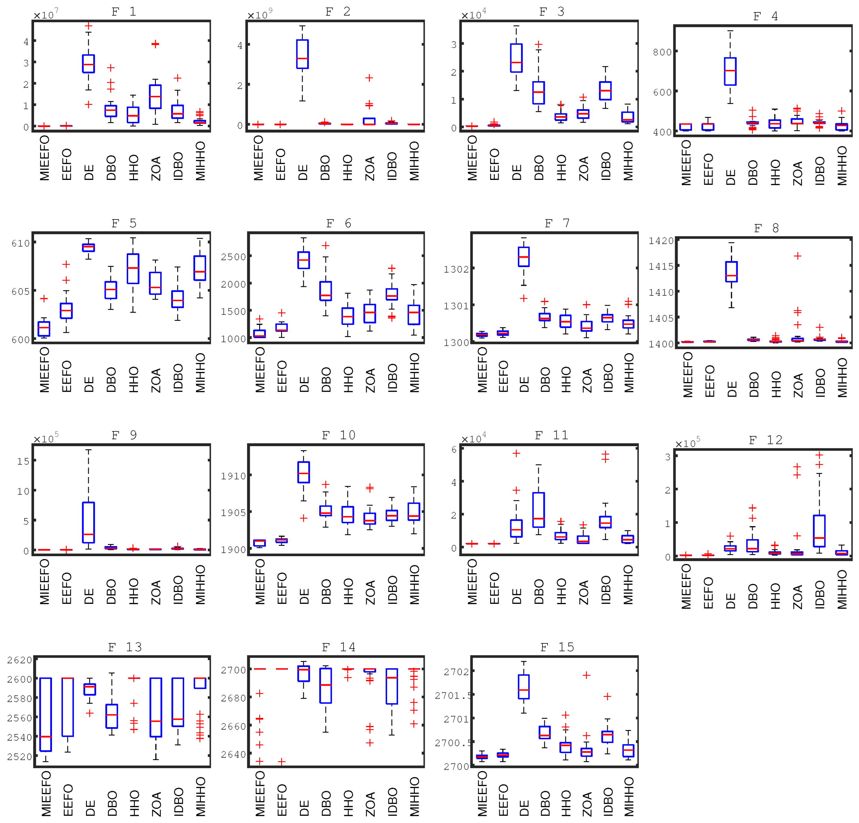
This paper proposes an improved Electric Eel Optimization Algorithm (MIEEFO) and tests it on 15 benchmark functions. MIEEFO is compared with EEFO, DE, DBO, HHO, ZOA, IDBO and MIHHO. The experimental results clearly demonstrate that MIEEFO exhibits superior exploration, exploitation, robustness and convergence accuracy. Additionally, MIEEFO is applied to the problem of color image segmentation. The test images include benchmark color images from the Berkeley database and forest fire images from real-world engineering problems. Using Kapur’s entropy as the fitness function, MIEEFO is compared with EEFO, LHHO, NHHGWO, HSMAWOA and HVSFA under different threshold levels. The experimental results show that the segmentation algorithm based on MIEEFO outperforms other algorithms across various threshold levels, proving the effectiveness of the model.
In future work, our research will focus on the following aspects: On the one hand, while the algorithm has already produced reliable results, additional strategies can be incorporated to further balance exploration and exploitation capabilities, thereby enhancing the convergence speed of EEFO. On the other hand, the improved MIEEFO can be applied to more complex domains, such as power systems, feature selection, data mining, artificial intelligence and other benchmark functions.

Author Contributions

Y.H. and L.Z. contributed to the idea of this paper; Y.H. performed the experiments; all authors analyzed data; Y.H. wrote the manuscript; Y.H., L.Z. and H.Z. contributed to the revision of the manuscript. All authors have read and agreed to the published version of the manuscript.

Funding

This research was funded by the The Central Government guides the local Science and Technology Development Project (ZY24QY03), the national key research and development Project (2021YFC2202502), the central university basic research funds special fund (2021YFC2202502).

Data Availability Statement

Data are contained within the article.

Acknowledgments

The authors thank the anonymous reviewers for their useful comments, which improved the quality of the paper.

Conflicts of Interest

The authors declare no conflicts of interest.

References

  1. Yu, Y.; Wang, C.; Fu, Q.; Kou, R.; Huang, F.; Yang, B.; Yang, T.; Gao, M. Techniques and challenges of image segmentation: A review. Electronics 2023, 12, 1199. [Google Scholar] [CrossRef]
  2. Reda, M.; Onsy, A.; Haikal, A.Y.; Ghanbari, A. Path planning algorithms in the autonomous driving system: A comprehensive review. Robot. Auton. Syst. 2024, 174, 104630. [Google Scholar] [CrossRef]
  3. Shaikh, P.W.; El-Abd, M.; Khanafer, M.; Gao, K.Z. A review on swarm intelligence and evolutionary algorithms for solving the traffic signal control problem. IEEE Trans. Intell. Transp. Syst. 2022, 23, 48–63. [Google Scholar] [CrossRef]
  4. Zivkovic, M.; Bacanin, N.; Venkatachalam, K.; Nayyar, A.; Djordjevic, A.; Strumberger, I.; Al-Turjman, F. COVID-19 cases prediction by using hybrid machine learning and beetle antennae search approach. Sustain. Cities Soc. 2021, 66, 102669. [Google Scholar] [CrossRef] [PubMed]
  5. Qin, J.; Hu, F.; Liu, Y.; Witherell, P.; Wang, C.C.L.; Rosen, D.W.; Simpson, T.W.; Lu, Y.; Tang, Q. Research and application of machine learning for additive manufacturing. Addit. Manuf. 2022, 52, 102691. [Google Scholar] [CrossRef]
  6. Han, J.; Yang, C.; Zhou, X.; Gui, W. A new multi-threshold image segmentation approach using state transition algorithm. Appl. Math. Model. 2017, 44, 588–601. [Google Scholar] [CrossRef]
  7. Liu, D.; Liang, B.; Li, J.; Lopez Estrada, F.R. Color uav image edge detection based on improved fireworks algorithm. Int. J. Aerosp. Eng. 2023, 1–12. [Google Scholar] [CrossRef]
  8. Aksac, A.; Ozyer, T.; Alhajj, R. Complex networks driven salient region detection based on superpixel segmentation. Pattern Recognit. 2017, 66, 268–279. [Google Scholar] [CrossRef]
  9. Narayanan, B.N.; Hardie, R.C.; Kebede, T.M.; Sprague, M.J. Optimized feature selection-based clustering approach for computer-aided detection of lung nodules in different modalities. Pattern Anal. Appl. 2019, 22, 559–571. [Google Scholar] [CrossRef]
  10. Ahmadi, A.; Karray, F.; Kamel, M.S. Model order selection for multiple cooperative swarms clustering using stability analysis. Inf. Sci. 2012, 182, 169–183. [Google Scholar] [CrossRef]
  11. Shelar, A.; Kulkarni, R. Analysis and design of optimal deep neural network model for image recognition using hybrid cuckoo search with self-adaptive particle swarm intelligence. Signal Image Video Process. 2024, 18, 6987–6995. [Google Scholar] [CrossRef]
  12. Devarajan, G.G.; Nagarajan, S.M.; Daniel, A.; Vignesh, T.; Kaluri, R. Consumer product recommendation system using adapted pso with federated learning method. IEEE Trans. Consum. Electron. 2024, 70, 2708–2715. [Google Scholar]
  13. Ren, L.; Heidari, A.A.; Cai, Z.; Shao, Q.; Liang, G.; Chen, H.L.; Pan, Z. Gaussian kernel probability-driven slime mould algorithm with new movement mechanism for multi-level image segmentation. Measurement 2022, 192, 110884. [Google Scholar]
  14. Naik, M.K.; Panda, R.; Wunnava, A.; Jena, B.; Abraham, A. A leader harris hawks optimization for 2-d masi entropy-based multilevel image thresholding. Multimed. Tools Appl. 2021, 80, 35543–35583. [Google Scholar]
  15. Bhandari, A.K.; Kumar, A.; Singh, G.K. Modified artificial bee colony based computationally efficient multilevel thresholding for satellite image segmentation using kapur’s, otsu and tsallis functions. Expert Syst. Appl. 2015, 42, 1573–1601. [Google Scholar]
  16. Fan, Q.; Ma, Y.; Wang, P.; Bai, F. Otsu image segmentation based on a fractional order moth–flame optimization algorithm. Fractal Fract. 2024, 8, 87. [Google Scholar] [CrossRef]
  17. Guo, Y.; Wang, Y.; Meng, K.; Zhu, Z. Otsu multi-threshold image segmentation based on adaptive double-mutation differential evolution. Biomimetics 2023, 8, 418. [Google Scholar] [CrossRef]
  18. Shajin, F.H.; Aruna Devi, B.; Prakash, N.B.; Sreekanth, G.R.; Rajesh, P. Sailfish optimizer with levy flight, chaotic and opposition-based multi-level thresholding for medical image segmentation. Soft Comput. 2023, 27, 12457–12482. [Google Scholar]
  19. Zhang, H.; Cai, Z.; Xiao, L.; Heidari, A.A.; Chen, H.; Zhao, D.; Wang, S.; Zhang, Y. Face image segmentation using boosted grey wolf optimizer. Biomimetics 2023, 8, 484. [Google Scholar] [CrossRef]
  20. Sharma, A.; Chaturvedi, R.; Bhargava, A. A novel opposition based improved firefly algorithm for multilevel image segmentation. Multimed. Tools Appl. 2022, 81, 15521–15544. [Google Scholar] [CrossRef]
  21. Khosla, T.; Verma, O.P. Optimal threshold selection for segmentation of chest x-ray images using opposition-based swarm-inspired algorithm for diagnosis of pneumonia. Multimed. Tools Appl. 2024, 83, 27089–27119. [Google Scholar]
  22. Oliva, D.; Zhang, C.; Pei, Y.H.; Wang, X.X.; Hou, H.Y.; Fu, L.H. Symmetric cross-entropy multi-threshold color image segmentation based on improved pelican optimization algorithm. PLoS ONE 2023, 18, e0287573. [Google Scholar]
  23. Dhal, K.G.; Das, A.; Ray, S.; Galvez, J.; Das, S. Nature-inspired optimization algorithms and their application in multi-thresholding image segmentation. Arch. Comput. Methods Eng. 2020, 27, 855–888. [Google Scholar]
  24. Houssein, E.H.; Emam, M.M.; Ali, A.A. An efficient multilevel thresholding segmentation method for thermography breast cancer imaging based on improved chimp optimization algorithm. Expert Syst. Appl. 2021, 185, 115651. [Google Scholar] [CrossRef]
  25. Sabha, M.; Thaher, T.; Emam, M.M. Cooperative swarm intelligence algorithms for adaptive multilevel thresholding segmentation of COVID-19 ct-scan images. JUCS-J. Univers. Comput. Sci. 2023, 29, 759–804. [Google Scholar]
  26. Hao, S.; Huang, C.; Heidari, A.A.; Chen, H.; Li, L.; Algarni, A.D.; Elmannai, H.; Xu, S. Salp swarm algorithm with iterative mapping and local escaping for multi-level threshold image segmentation: A skin cancer dermoscopic case study. J. Comput. Des. Eng. 2023, 10, 655–693. [Google Scholar]
  27. Chauhan, D.; Yadav, A. A crossover-based optimization algorithm for multilevel image segmentation. Soft Comput. 2023. [CrossRef]
  28. Qian, Y.; Tu, J.; Luo, G.; Sha, C.; Heidari, A.A.; Chen, H. Multi-threshold remote sensing image segmentation with improved ant colony optimizer with salp foraging. J. Comput. Des. Eng. 2023, 10, 2200–2221. [Google Scholar] [CrossRef]
  29. Dhal, K.G.; Ray, S.; Barik, S.; Das, A. Illumination-free clustering using improved slime mould algorithm for acute lymphoblastic leukemia image segmentation. J. Bionic Eng. 2023, 20, 2916–2934. [Google Scholar]
  30. Shi, J.; Chen, Y.; Wang, C.; Heidari, A.A.; Liu, L.; Chen, H.; Chen, X.; Sun, L. Multi-threshold image segmentation using new strategies enhanced whale optimization for lupus nephritis pathological images. Displays 2024, 84, 102799. [Google Scholar]
  31. Houssein, E.H.; Mohamed, G.M.; Samee, N.A.; Alkanhel, R.; Ibrahim, I.A.; Wazery, Y.M. An improved search and rescue algorithm for global optimization and blood cell image segmentation. Diagnostics 2023, 13, 1422. [Google Scholar] [CrossRef]
  32. Wu, B.; Zhu, L.; Li, X. Giza pyramids construction algorithm with gradient contour approach for multilevel thresholding color image segmentation. Appl. Intell. 2023, 53, 21248–21267. [Google Scholar] [CrossRef]
  33. Kennedy, J.; Eberhart, R. Particle swarm optimization. In Proceedings of the ICNN’95-International Conference on Neural Networks, Perth, WA, Australia, 27 November–1 December 1995; IEEE: Piscataway, NJ, USA, 1995; Volume 4, pp. 1942–1948. [Google Scholar]
  34. Nadimi-Shahraki, M.H.; Taghian, S.; Mirjalili, S.; Faris, H. Mtde: An effective multi-trial vector-based differential evolution algorithm and its applications for engineering design problems. Appl. Soft Comput. 2020, 97, 106761. [Google Scholar] [CrossRef]
  35. Karaboga, D.; Akay, B. A comparative study of artificial bee colony algorithm. Appl. Math. Comput. 2009, 214, 108–132. [Google Scholar] [CrossRef]
  36. Mirjalili, S.; Lewis, A. The whale optimization algorithm. Adv. Eng. Softw. 2016, 95, 51–67. [Google Scholar] [CrossRef]
  37. Zhao, W.; Wang, L.; Zhang, Z.; Fan, H.; Zhang, J.; Mirjalili, S.; Khodadadi, N.; Cao, Q. Electric eel foraging optimization: A new bio-inspired optimizer for engineering applications. Expert Syst. Appl. 2024, 238, 122200. [Google Scholar] [CrossRef]
  38. Abualigah, L.; Diabat, A.; Mirjalili, S.; Elaziz, M.A.; Gandomi, A.H. The arithmetic optimization algorithm. Comput. Methods Appl. Mech. Eng. 2021, 376, 113609. [Google Scholar] [CrossRef]
  39. Alabool, H.M.; Alarabiat, D.; Abualigah, L.; Heidari, A.A. Harris hawks optimization: A comprehensive review of recent variants and applications. Neural Comput. Appl. 2021, 33, 8939–8980. [Google Scholar] [CrossRef]
  40. Zhong, C.; Li, G.; Meng, Z. Beluga whale optimization: A novel nature-inspired metaheuristic algorithm. Knowl.-Based Syst. 2022, 251, 109215. [Google Scholar] [CrossRef]
  41. Wolpert, D.; Macready, W. No free lunch theorems for optimization. IEEE Trans. Evol. Comput. 1997, 1, 67–82. [Google Scholar]
  42. Liu, R.; Wang, T.; Zhou, J.; Hao, X.; Xu, Y.; Qiu, J. Improved african vulture optimization algorithm based on quasi-oppositional differential evolution operator. IEEE Access 2022, 10, 95197–95218. [Google Scholar]
  43. Tizhoosh, H.R. Opposition-based learning: A new scheme for machine intelligence. In Proceedings of the International Conference on Computational Intelligence for Modelling, Control and Automation and International Conference on Intelligent Agents, Web Technologies and Internet Commerce (CIMCA-IAWTIC’06), Vienna, Austria, 28–30 November 2005; IEEE: Piscataway, NJ, USA, 2005; Volume 1, pp. 695–701. [Google Scholar]
  44. Loganathan, V.; Veerappan, S.; Manoharan, P.; Derebew, B. Optimizing drone-based iot base stations in 6g networks using the quasi-opposition-based lemurs optimization algorithm. Int. J. Comput. Intell. Syst. 2024, 17, 218. [Google Scholar]
  45. Shan, W.; He, X.; Liu, H.; Heidari, A.A.; Wang, M.; Cai, Z.; Chen, H. Cauchy mutation boosted harris hawk algorithm: Optimal performance design and engineering applications. J. Comput. Des. Eng. 2023, 10, 503–526. [Google Scholar] [CrossRef]
  46. Xue, J.K.; Shen, B. Dung beetle optimizer: A new meta-heuristic algorithm for global optimization. J. Supercomput. 2023, 79, 7305–7336. [Google Scholar] [CrossRef]
  47. Trojovska, E.; Dehghani, M.; Trojovsky, P. Zebra optimization algorithm: A new bio-inspired optimization algorithm for solving optimization algorithm. IEEE Access 2022, 10, 49445–49473. [Google Scholar] [CrossRef]
  48. Wu, Q.; Xu, H.; Liu, M. Applying an improved dung beetle optimizer algorithm to network traffic identification. Comput. Mater. Contin. 2024, 78, 4091–4107. [Google Scholar]
  49. Li, C.Y.; Si, Q.; Zhao, J.A.; Qin, P.B. A robot path planning method using improved harris hawks optimization algorithm. Meas. Control. 2024, 57, 469–482. [Google Scholar] [CrossRef]
  50. Cai, J.; Luo, T.; Xu, G.; Tang, Y. A novel biologically inspired approach for clustering and multi-level image thresholding: Modified harris hawks optimizer. Cogn. Comput. 2022, 14, 955–969. [Google Scholar] [CrossRef]
  51. Abdel-Basset, M.; Chang, V.; Mohamed, R. optimization algorithm for tackling the image segmentation problem of chest X-ray images. Appl. Soft Comput. 2020, 95, 106642. [Google Scholar]
  52. Chen, Y.; Wang, M.; Heidari, A.A.; Shi, B.; Hu, Z.; Zhang, Q.; Chen, H.; Mafarja, M.; Turabieh, H. Multi-threshold image segmentation using a multi-strategy shuffled frog leaping algorithm. Expert Syst. Appl. 2022, 194, 116511. [Google Scholar] [CrossRef]
  53. Paygude, S.; Vyas, V. Dynamic texture segmentation approaches for natural and manmade cases: Survey and experimentation. Arch. Comput. Methods Eng. 2020, 27, 285–297. [Google Scholar] [CrossRef]
Figure 1. Physical structure and electricity producing organs of electric eels.
Mathematics 13 01212 g001
Figure 2. Flow chart of the proposed EEFO method.
Mathematics 13 01212 g002
Figure 3. Flow chart of the proposed MIEEFO method.
Mathematics 13 01212 g003
Figure 4. Convergence diagram of MIEEFO algorithm in test function.
Mathematics 13 01212 g004
Figure 5. Function box diagram test.
Mathematics 13 01212 g005
Figure 6. The original image and corresponding histograms for each color channel (red, green, blue).
Mathematics 13 01212 g006
Figure 7. Four threshold level values for PSNR evaluation.
Mathematics 13 01212 g007
Figure 8. Four threshold level values for SSIM evaluation.
Mathematics 13 01212 g008
Figure 9. Four threshold level values for FSIM evaluation.
Mathematics 13 01212 g009
Figure 10. Results of image segmentation with a threshold of 4.
Mathematics 13 01212 g010
Figure 11. Results of image segmentation with a threshold of 12.
Mathematics 13 01212 g011
Figure 12. Forest fire image.
Mathematics 13 01212 g012
Figure 13. Result of MIEEFO-based multilevel thresholding segmentation algorithm.
Mathematics 13 01212 g013
Table 1. Description of the test functions (search range: 100 , 100 ).
ClassFunctionDescription Fi
UnimodalF1Rotated High Conditioned Elliptic Function100
F2Rotated Bent Cigar Function200
F3Rotated Discus Function300
MultimodalF4Shifted and Rotated Rosenbrock’s Function400
F5Shifted and Rotated Weierstrass Function600
F6Shifted Schwefel’s Function1000
F7Shifted and Rotated HappyCat Function1300
F8Shifted and Rotated HGBat Function1400
HybridF9Hybrid Function 21800
F10Hybrid Function 31900
F11Hybrid Function 42000
F12Hybrid Function 52100
CompositionF13Composition Function 22400
F14Composition Function 32500
F15Composition Function 42600
Table 2. Algorithm parameter settings.
AlgorithmParameters
MIEEFO fi = 1.5 , TR = 0.3  F = 0.5,  C r = 0.9
EEFO β = 1.5
DEF = 0.5,  C r = 0.9
DBOk = 0.1, b = 0.3,  ff = 1
HHO E 0 ϵ 1 , 1
ZOAl ϵ 1 , 2
IDBOk = 0.1, b = 0.3, ff = 1
MIHHO fi = 1.5
Table 3. The experimental results of different algorithms on the test functions.
ID MIEEFOEEFODEDBOHHOZOAIDBOMIHHO
F1Mean498.033.33 ×   10 4 2.82 ×   10 7 7.99 ×   10 6 8.18 ×   10 6 1.46 ×   10 7 9.62 ×   10 6 2.93 ×   10 6
Std437.554.80 ×   10 4 9.52 ×   10 6 3.23 ×   10 6 6.03 ×   10 6 9.46 ×   10 6 4.78 ×   10 6 2.48 ×   10 6
F2Mean1914.022005.423.19 × 1094.80 ×   10 7 3.47 ×   10 5 2.32 × 1085.10 ×   10 7 2.62 ×   10 5
Std2111.582200.189.45 × 1082.70 ×   10 7 1.36 ×   10 5 3.57 × 1082.51 ×   10 7 9.28 ×   10 4
F3Mean300.08520.342.28 ×   10 4 1.32 ×   10 4 4101.364695.3012077.083920.48
Std0.11277.735829.806082.421832.582611.163881.981820.69
F4Mean413.91418.70704.47443.22436.04449.91443.75432.74
Std15.9616.2876.7126.6416.0237.6914.1924.73
F5Mean600.91602.40609.51605.22607.32605.90604.73606.97
Std0.711.100.801.381.811.621.371.57
F6Mean1105.261148.692476.301926.611492.781421.381777.991304.50
Std92.38123.62159.93321.87256.26187.79243.82183.96
F7Mean1300.181300.231302.281300.671300.521300.451300.631300.58
Std0.060.090.310.170.160.200.190.25
F8Mean1400.221400.251414.711400.711400.341401.311400.601400.22
Std0.070.102.830.220.312.740.200.07
F9Mean1804.732516.834.20 ×   10 5 4.48 ×   10 4 9889.6078552.732.71 ×   10 4 1.05 ×   10 4
Std2.532344.314.23 ×   10 5 4.71 ×   10 4 4150.3973926.932.58 ×   10 4 7929.32
F10Mean1900.771901.071910.211905.051904.451906.011904.8481905.10
Std0.370.482.270.941.247.460.991.61
F11Mean2001.942004.491.17 ×   10 4 2.12 ×   10 4 6142.065650.5815657.614365.96
Std1.263.375909.7041.50 ×   10 4 3090.362220.308158.861861.18
F12Mean2109.192233.662.43 ×   10 4 5.70 ×   10 4 9984.146.70 ×   10 4 4.28 ×   10 4 1.32 ×   10 4
Std11.92167.042.00 ×   10 4 5.43 ×   10 4 7232.611.03 ×   10 5 4.00 ×   10 4 1.05 ×   10 4
F13Mean2550.662563.342585.912569.802594.192563.052570.752583.15
Std31.4832.6610.0418.6313.8030.8720.9725.62
F14Mean2689.462696.112696.152692.712699.652694.862689.602697.14
Std16.2412.728.4312.451.9112.6314.5910.57
F15Mean2700.162700.182701.782700.592700.362700.362700.612700.38
Std0.050.050.380.100.170.380.120.15
FriedmanAvg1.75222.50677.22895.62224.65674.51335.47224.2478
Rank12875463
Table 4. Wilcoxon test results.
FunctionEEFODEDBOHHOZOAIDBOMIHHO
F15.87 ×   10 10 1.51 ×   10 11 1.51 ×   10 11 1.51 ×   10 11 1.51 ×   10 11 1.51 ×   10 11 1.51 ×   10 11
F25.00 ×   10 2 1.51 ×   10 11 1.51 ×   10 11 1.51 ×   10 11 1.02 ×   10 9 1.51 ×   10 11 1.51 ×   10 11
F31.51 ×   10 11 1.51 ×   10 11 1.51 ×   10 11 1.51 ×   10 11 1.51 ×   10 11 1.51 ×   10 11 1.51 ×   10 11
F42.11 ×   10 4 1.51 ×   10 11 2.37 ×   10 6 3.87 ×   10 6 4.42 ×   10 7 8.47 ×   10 10 3.18 ×   10 5
F51.66 ×   10 6 1.51 ×   10 11 1.51 ×   10 11 1.51 ×   10 11 1.51 ×   10 11 1.51 ×   10 11 1.51 ×   10 11
F65.00 ×   10 2 1.51 ×   10 11 1.51 ×   10 11 1.42 ×   10 8 1.11 ×   10 9 1.51 ×   10 11 2.59 ×   10 7
F75.00 ×   10 2 1.51 ×   10 11 1.51 ×   10 11 1.51 ×   10 11 2.37 ×   10 6 1.51 ×   10 11 9.28 ×   10 10
F86.51 ×   10 4 1.51 ×   10 11 1.51 ×   10 11 5.00 ×   10 2 2.73 ×   10 9 1.51 ×   10 11 3.81 ×   10 3
F92.49 ×   10 11 1.51 ×   10 11 1.51 ×   10 11 1.51 ×   10 11 1.51 ×   10 11 1.51 ×   10 11 1.51 ×   10 11
F101.14 ×   10 5 1.51 ×   10 11 1.51 ×   10 11 1.51 ×   10 11 1.51 ×   10 11 1.51 ×   10 11 1.51 ×   10 11
F113.37 ×   10 6 1.51 ×   10 11 1.51 ×   10 11 1.51 ×   10 11 1.51 ×   10 11 1.51 ×   10 11 1.51 ×   10 11
F123.52 ×   10 7 1.51 ×   10 11 1.51 ×   10 11 1.51 ×   10 11 1.51 ×   10 11 1.51 ×   10 11 1.51 ×   10 11
F131.53 ×   10 2 3.93 ×   10 3 3.60 ×   10 3 1.31 ×   10 7 1.72 ×   10 3 1.77 ×   10 2 1.26 ×   10 3
F142.08 ×   10 2 5.00 ×   10 2 5.00 ×   10 2 5.00 ×   10 2 5.00 ×   10 2 5.00 ×   10 2 5.00 ×   10 2
F152.63 ×   10 5 1.51 ×   10 11 1.51 ×   10 11 1.84 ×   10 11 1.30 ×   10 5 1.51 ×   10 11 2.09 ×   10 9
+/=/−12/3/013/1/014/1/013/2/014/1/014/1/014/1/0
Table 5. PSNR values for each method.
ImageDimMIEEFOEEFOLHHONHHGWOHSMAWOAHVSFLA
Image1421.523721.505421.523721.453421.523720.4470
622.878022.090522.142322.700222.819322.5626
824.522624.048824.177124.156324.137724.0919
1226.522526.471026.197825.924526.217826.3472
Image2420.922420.922420.891020.779420.891020.9200
622.591222.540322.368022.467322.565822.5770
824.510524.491524.461124.414624.360724.4154
1228.313028.224728.229728.007728.141827.9479
Image3418.274318.274318.274318.357718.274318.2925
621.336121.164321.330721.304021.330721.3275
823.539723.508123.482023.446223.439423.5385
1227.748827.615727.663427.206427.678827.6355
Image4419.659319.638919.657019.520419.657219.6572
623.089723.044623.078022.856923.087422.9759
824.051923.946924.048123.714923.860024.0359
1227.762827.456227.539227.317427.752727.3130
Image5419.660619.660619.660619.633819.660619.6464
621.475321.468521.421719.633821.451221.4498
824.074823.937524.034023.688223.923923.9936
1227.585527.528027.544127.426127.513927.5788
Image6418.556018.556018.556018.543718.556018.5541
621.295121.290521.294721.237621.294721.2807
823.630323.602523.602523.330223.625223.5916
1227.138127.089627.041926.959627.069827.1381
Table 6. SSIM values for each method.
ImageDimMIEEFOEEFOLHHONHHGWOHSMAWOAHVSFLA
Image140.66730.66140.66180.66180.66180.6268
60.72460.71730.71760.72460.71770.7075
80.78230.77340.77200.77600.78190.7814
120.83910.83910.83720.82550.83190.8350
Image240.86070.86070.85940.86060.85940.8564
60.89200.88720.88570.88650.88600.8874
80.91750.91630.91430.91590.91270.9162
120.93780.93200.93340.93550.93550.9358
Image340.68880.68690.68690.68870.68690.6869
60.80250.80210.80230.80220.80220.8016
80.86100.86010.85870.85540.85860.8586
120.93240.93090.93090.91670.92780.9323
Image440.88430.88400.88420.88400.88430.8840
60.91480.91470.91440.91450.91480.9147
80.92410.92310.92230.92030.92310.9238
120.92800.92670.92600.92200.92790.9274
Image540.54070.54070.54070.53950.54070.5407
60.59560.58650.58590.62460.58690.5869
80.67390.67300.67320.67310.66820.6716
120.80150.79330.79210.80960.79010.7883
Image640.68540.68540.68540.67960.68540.6555
60.75740.75730.75700.75680.75700.7562
80.82070.81960.81960.81090.81960.8199
120.89890.89810.88800.89330.89740.8799
Table 7. FSIM values for each method.
ImageDimMIEEFOEEFOLHHONHHGWOHSMAWOAHVSFLA
Image140.79450.79440.79450.79300.79450.7700
60.83040.81460.80740.81460.82260.8244
80.85920.85890.85790.85770.85910.8546
120.90890.90780.90530.90830.90660.9053
Image240.85360.85330.85250.85330.85250.8533
60.87480.87480.87030.87310.87470.8748
80.89160.89150.89100.89160.88960.8915
120.92120.91810.91980.91700.91900.9208
Image340.79330.79260.79260.79240.79260.7926
60.87060.87020.87050.86690.87030.8703
80.91090.90830.90790.90980.90810.9084
120.95860.95720.95780.95550.95360.9577
Image440.87770.87770.87760.87750.87770.8774
60.90340.90330.90330.90310.90250.9024
80.91590.91570.91520.91500.91560.9141
120.93420.93350.93830.93360.93410.9310
Image540.72190.72190.72190.72070.72190.7120
60.77090.77030.77020.75560.76100.7608
80.80460.80390.80290.80020.80210.8032
120.87930.87700.87920.87820.87710.8745
Image640.81210.81200.81200.81190.81200.8121
60.86780.86760.86750.86270.86750.8742
80.90460.90440.90400.90210.90400.9040
120.94380.94350.94350.94160.94330.9435
Table 8. PSNR values for each method.
ImageDimMEEFOEEFOLHHONHHGWOHSMAWOAHVSFLA
Image729.82339.82339.82339.82339.82339.8233
418.847318.847318.808218.753218.847318.8473
824.498124.453624.436724.448624.469524.0293
1026.758326.742926.680525.861526.694826.5086
1228.136028.094827.833727.320128.057128.0438
Image8210.380510.380510.380510.380510.380510.3805
418.910418.910418.910418.087318.910418.9104
824.900124.811724.742524.035824.708824.5550
1026.752826.662126.714525.601426.608926.4455
1227.840727.693527.701926.761627.544527.6708
Table 9. SSIM values for each method.
ImageDimMEEFOEEFOLHHONHHGWOHSMAWOAHVSFLA
Image720.28390.28390.28390.28390.28390.2839
40.64740.64740.64740.63230.64740.6474
80.81610.81280.81370.81340.81560.8123
100.86590.86300.86300.85230.86380.8572
120.89110.88980.88520.88440.88240.8877
Image820.29530.29530.29530.29530.29530.2953
40.65540.65540.65540.64210.65540.6554
80.83830.83750.83160.83460.83610.8365
100.88160.87090.87900.85730.87480.8810
120.90180.89090.89240.87550.88950.8991
Table 10. FSIM values for each method.
ImageDimMEEFOEEFOLHHONHHGWOHSMAWOAHVSFLA
Image720.63830.63830.63830.63600.63830.6383
40.81390.81390.81170.81270.81000.8139
80.91120.91090.91100.90720.91050.9012
100.94910.94780.94880.93480.94880.9446
120.96290.96190.96100.95440.96110.9602
Image820.64360.64360.64360.64360.64360.6436
40.82560.82240.82240.81590.82240.8224
80.92150.91950.91930.91740.91690.9112
100.95140.95020.95050.93800.94960.9513
120.96450.96250.96420.94650.95950.9604
Disclaimer/Publisher’s Note: The statements, opinions and data contained in all publications are solely those of the individual author(s) and contributor(s) and not of MDPI and/or the editor(s). MDPI and/or the editor(s) disclaim responsibility for any injury to people or property resulting from any ideas, methods, instructions or products referred to in the content.

