
Feedforward Factorial Hidden Markov Model

Abstract
1. Introduction
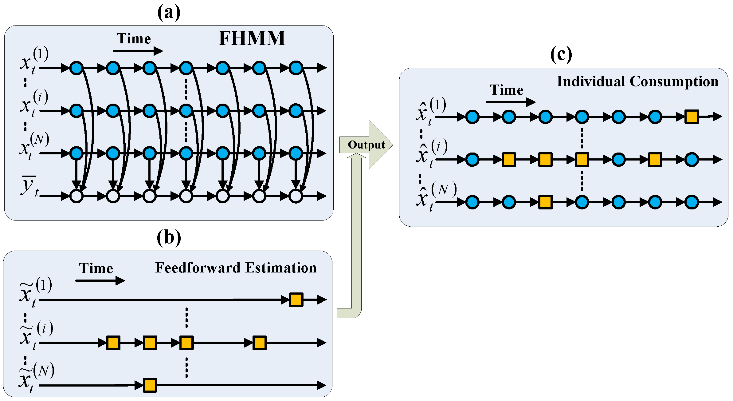
2. Feedforward FHMM
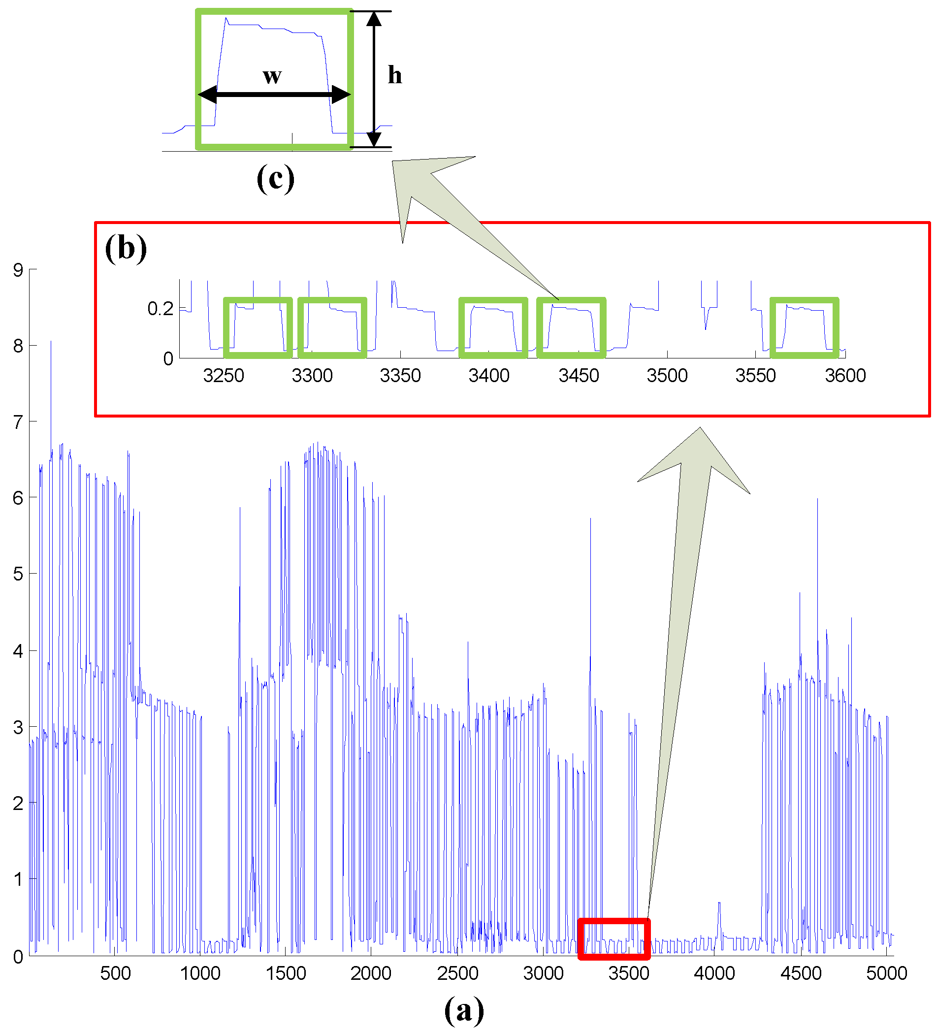
2.1. Automatic Feature Filter
- If for all such that , we have , then
- Otherwise,
2.2. Direct FFHMM
| Algorithm 1: EXACT algorithm for direct FFHMM | |
| 1 | Initialization: . |
| 2 | Recursion: . |
| 3 | Termination: |
| 4 | Path backtracking: |
| 5 | Merging: |
| Algorithm 2: AFAMAP algorithm for direct FFHMM | |
| 1 | Input: , , , , , and . |
| 2 | Minimization: |
| 3 | Output: , predicted the output of individual HMM |
- Firstly, it simplifies the control over outcomes for a designated HMM chain. Specifically, as the AFF’s estimations directly supersede those of the FHMM during particular timeframes, the accuracy of the FFHMM for the target HMM chain is unlikely to decline, assuming the AFF’s accuracy is maintained with sufficient conservatism. Secondly, an aggressive AFF can be employed to enhance the performance of the target HMM chain, though this approach carries a risk of potentially exacerbating outcomes.
- Secondly, alterations in accuracy for the estimation of one HMM chain are independent of changes in others. This attribute facilitates the independent improvement in accuracy for each HMM chain. Additionally, customized AFFs can be applied to specific HMM chains, thereby achieving superior results.
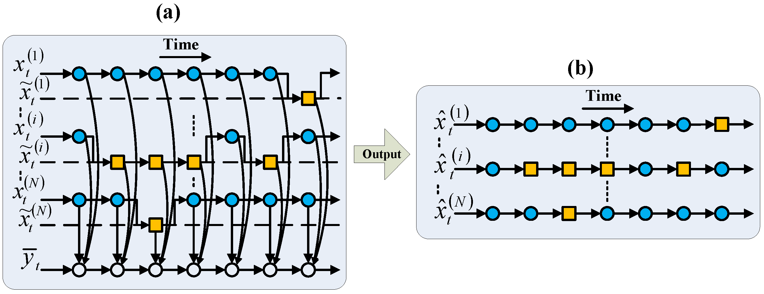
2.3. Embedded FFHMM
- 1.
- The initial state:
- (a)
- If , then
- (b)
- Otherwise,
- 2.
- The state transition:
- (a)
- If , then
- (b)
- Otherwise,
- 3.
- The observation probability distribution:
| Algorithm 3: EXACT algorithm for embedded FFHMM | |
| 1 | Initialization: , ,
|
| 2 | Recursion: , , , ,
|
| 3 | Termination: |
| 4 | Path backtracking: |
| Algorithm 4: AFAMAP algorithm for embedded FFHMM | |
| 1 | Input: , , , , , and . |
| 2 | Minimization: Output: , predicted individual HMM output |
3. Results
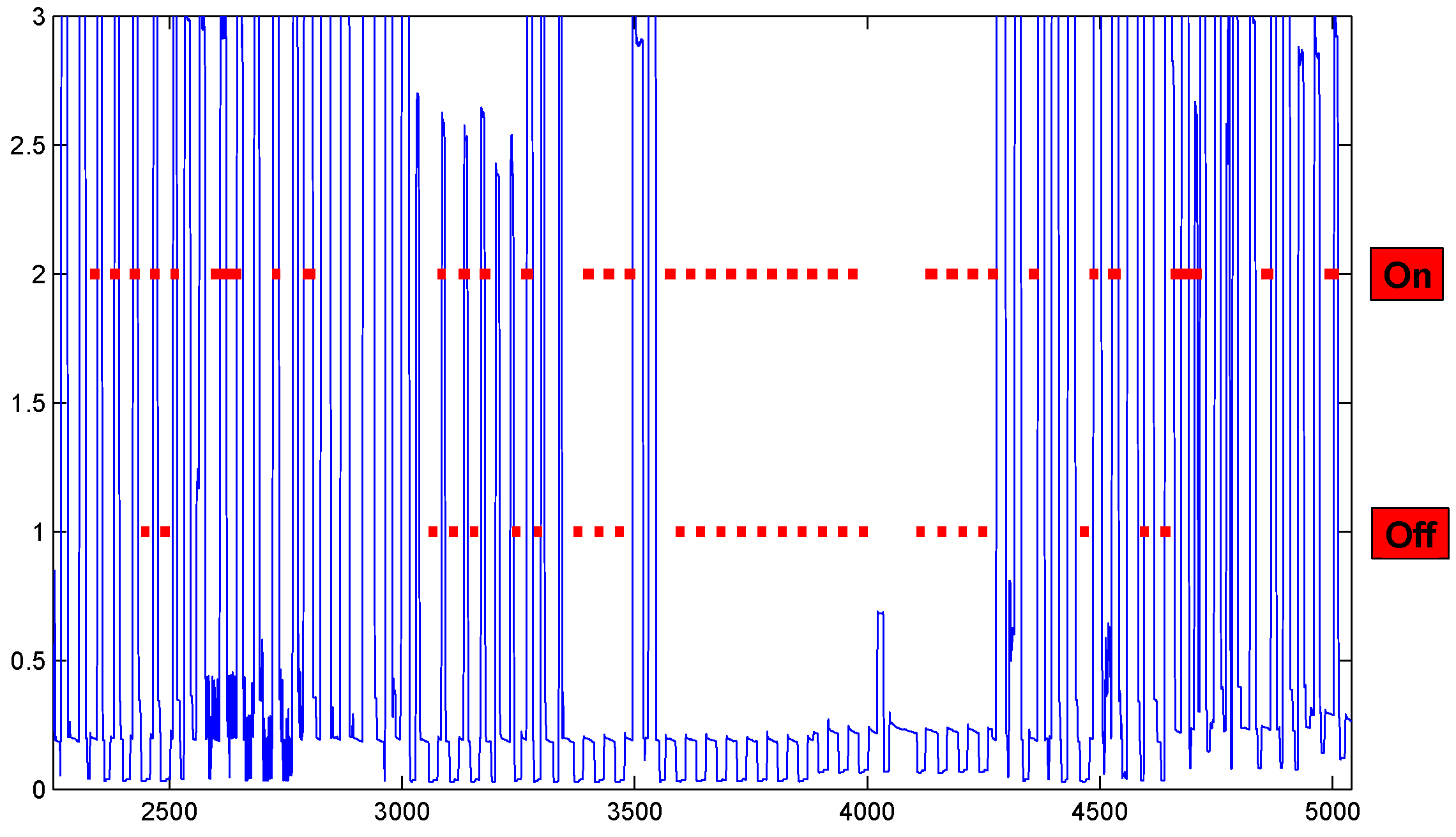
3.1. Automatic Pattern Recognition Using AFF
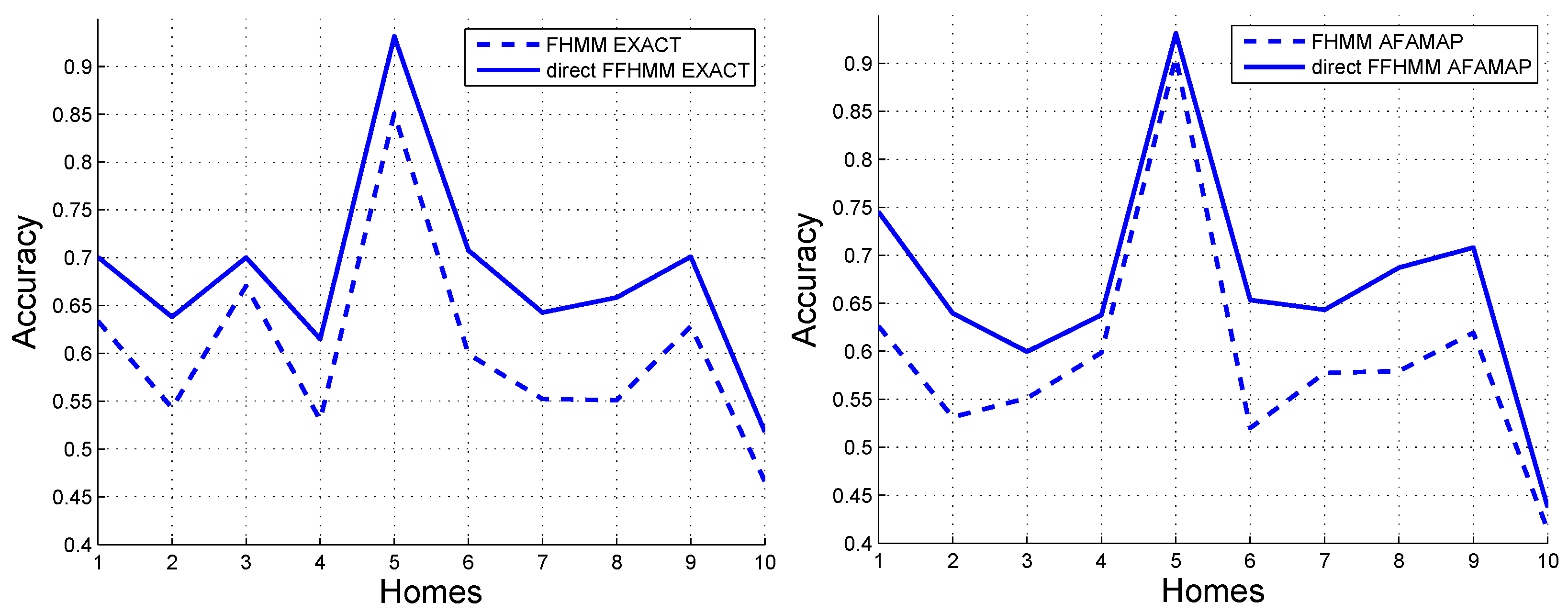
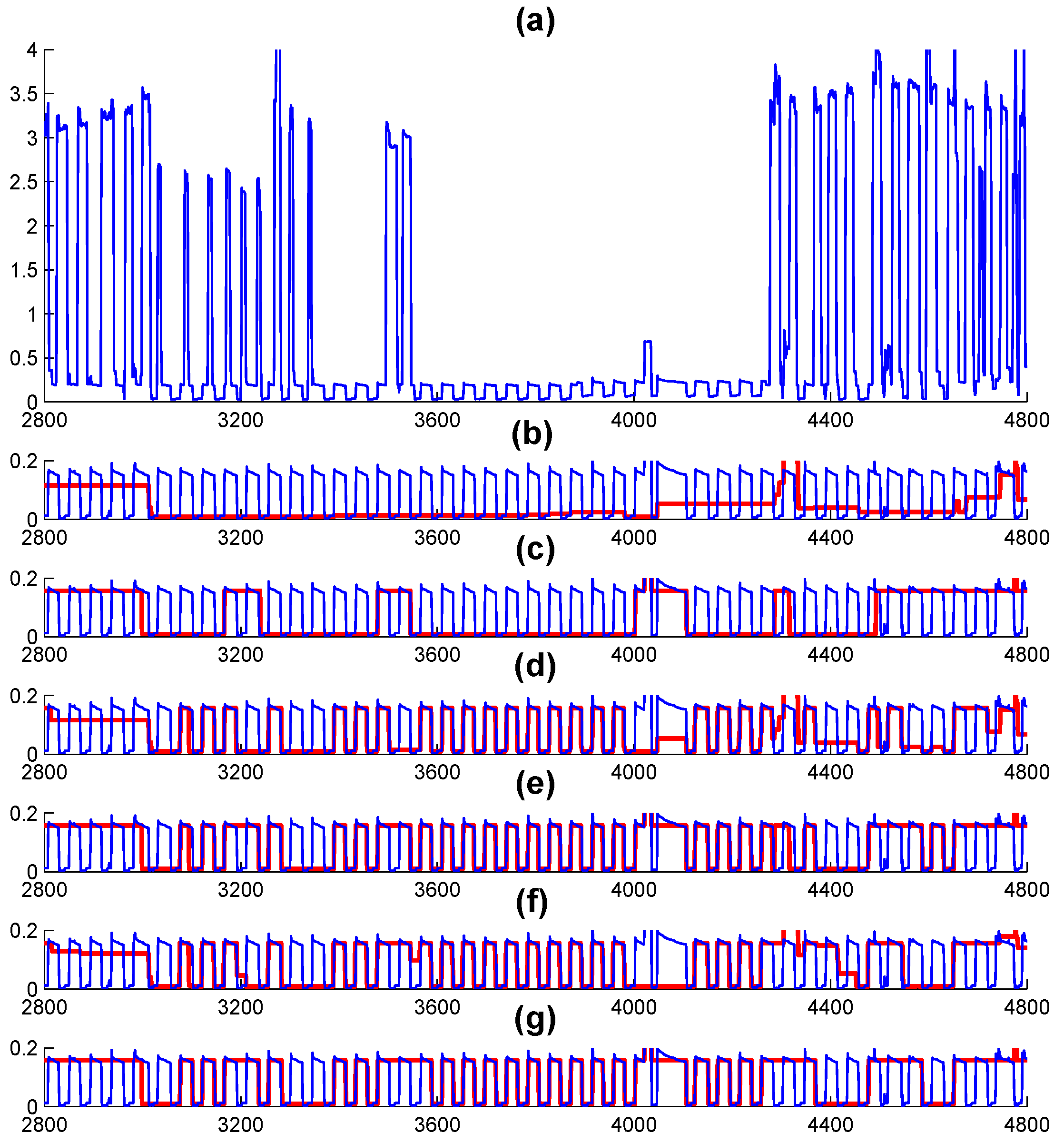
3.2. Experiments Using Direct FFHMM and Embedded FFHMM
4. Discussion
Author Contributions
Funding
Data Availability Statement
Acknowledgments
Conflicts of Interest
References
- Ghahramani, Z.; Jordan, M. Factorial hidden Markov models. Mach. Learn. 1997, 29, 245–273. [Google Scholar] [CrossRef]
- Schweiger, R.; Erlich, Y.; Carmi, S. FactorialHMM: Fast and exact inference in factorial hidden Markov models. Bioinformatics 2019, 35, 2162–2164. [Google Scholar] [CrossRef] [PubMed]
- Paeng, J.W.; Kwon, J. Visual tracking using interactive factorial hidden Markov models. IET Signal Process. 2021, 15, 365–374. [Google Scholar] [CrossRef]
- Kumar, P.; Abhyankar, A.R. A Time Efficient Factorial Hidden Markov Model-Based Approach for Non-Intrusive Load Monitoring. IEEE Trans. Smart Grid 2023, 14, 3627–3639. [Google Scholar] [CrossRef]
- Kani, A.; DeSarbo, W.S.; Fong, D.K. A factorial hidden Markov model for the analysis of temporal change in choice models. Cust. Needs Solut. 2018, 5, 162–177. [Google Scholar]
- Nepal, A.; Yates, A. Factorial Hidden Markov Models for Learning Representations of Natural Language. arXiv 2013, arXiv:1312.6168. [Google Scholar]
- Rahman, M.S.; Nicholson, A.E.; Haffari, G. HetFHMM: A Novel Approach to Infer Tumor Heterogeneity Using Factorial Hidden Markov Models. J. Comput. Biol. 2018, 25, 182–193. [Google Scholar] [CrossRef]
- Zhou, D.; Zhao, Y.; Wang, Z.; He, X.; Gao, M. Review on diagnosis techniques for intermittent faults in dynamic systems. IEEE Trans. Ind. Electron. 2019, 67, 2337–2347. [Google Scholar] [CrossRef]
- Duffield, S.; Power, S.; Rimella, L. A state-space perspective on modelling and inference for online skill rating. J. R. Stat. Soc. Ser. C Appl. Stat. 2024, 73, 1262–1282. [Google Scholar] [CrossRef]
- Puglisi, F.M.; Pavan, P. Factorial hidden Markov model analysis of random telegraph noise in resistive random access memories. ECTI Trans. Electr. Eng. Electron. Commun. 2014, 12, 24–29. [Google Scholar] [CrossRef]
- Saidane, M. Forecasting portfolio-Value-at-Risk with mixed factorial hidden Markov models. Croat. Oper. Res. Rev. 2019, 10, 241–255. [Google Scholar] [CrossRef]
- Durrieu, J.L.; Thiran, J.P. Source/filter factorial hidden markov model, with application to pitch and formant tracking. IEEE Trans. Audio Speech Lang. Process. 2013, 21, 2541–2553. [Google Scholar]
- Kolter, J.; Jaakkola, T. Approximate inference in additive factorial hmms with application to energy disaggregation. In Proceedings of the International Conference on Artificial Intelligence and Statistics, La Palma, Spain, 21–23 April 2012. [Google Scholar]
- Rabiner, L. A tutorial on Hidden Markov Models and selected applications in speech recognition. Proc. IEEE 1989, 77, 257–286. [Google Scholar]
- Chopin, N.; Papaspiliopoulos, O. An Introduction to Sequential Monte Carlo; Springer: Berlin/Heidelberg, Germany, 2020; Volume 4. [Google Scholar]
- Rebeschini, P.; Van Handel, R. Can local particle filters beat the curse of dimensionality? Ann. Appl. Probab. 2015, 25, 2809–2866. [Google Scholar] [CrossRef]
- Rimella, L.; Whiteley, N. Exploiting locality in high-dimensional Factorial hidden Markov models. J. Mach. Learn. Res. 2022, 23, 1–34. [Google Scholar]
- Franklin, G.F.; Powell, J.D.; Emami-Naeini, A. Feedback Control of Dynamic Systems, 8th ed.; Pearson: London, UK, 2018. [Google Scholar]
- Holcomb, C. Pecan Street Inc.: A test-bed for nilm. In Proceedings of the International Workshop on Non-Intrusive Load Monitoring, Pittsburgh, PA, USA, 7 May 2012. [Google Scholar]
- Kolter, J.; Johnson, M. REDD: A public data set for energy disaggregation research. In Proceedings of the Workshop on Data Mining Applications in Sustainability (SIGKDD), San Diego, CA, USA, 21 August 2011. [Google Scholar]
- Shao, H.; Marwah, M.; Ramakrishnan, N. A Temporal Motif Mining Approach to Unsupervised Energy Disaggregation: Applications to Residential and Commercial Buildings. In Proceedings of the Twenty-Seventh Conference on Artificial Intelligence (AAAI’13), Bellevue, WA, USA, 14–18 July 2013. [Google Scholar]
- Olson, D.; Delen, D. Advanced Data Mining Techniques, 1st ed.; Springer: Berlin/Heidelberg, Germany, 2008. [Google Scholar]


| No. of Home | Rate of Detection | Precision |
|---|---|---|
| 1 | 30.52% | 76.01% |
| 2 | 27.54% | 86.02% |
| 3 | 17.94% | 98.78% |
| 4 | 20.87% | 75.29% |
| 5 | 37.92% | 95.36% |
| 6 | 36.09% | 93.95% |
| 7 | 26.81% | 79.94% |
| 8 | 36.85% | 88.53% |
| 9 | 36.79% | 85.22% |
| 10 | 17.92% | 74.97% |
| Homes | Appliances | Ratio | FHMM | Embedded FFHMM | ||
|---|---|---|---|---|---|---|
| AFAMAP | EXACT | AFAMAP | EXACT | |||
| 1 | Refrigerator | 5.31% | 0.6262 | 0.6336 | 0.6749 | 0.7012 |
| Air conditioner 1 | 70.99% | 0.8417 | 0.9476 | 0.9387 | 0.9475 | |
| Furnace | 13.51% | 0.7580 | 0.7372 | 0.7645 | 0.7542 | |
| 2 | Refrigerator | 3.42% | 0.5315 | 0.5429 | 0.6344 | 0.5864 |
| Air conditioner 1 | 50.35% | 0.8096 | 0.9208 | 0.8106 | 0.9158 | |
| Furnace 1 | 27.29% | 0.9694 | 0.9589 | 0.9698 | 0.9608 | |
| Electrical dryer 1 | 6.74% | 0.5251 | 0.4955 | 0.5243 | 0.4008 | |
| Living room 1 | 5.47% | 0.2959 | 0.6970 | 0.3094 | 0.6491 | |
| 3 | Refrigerator | 8.84% | 0.5511 | 0.6706 | 0.6003 | 0.6831 |
| Air conditioner 1 | 45.60% | 0.8923 | 0.8975 | 0.8941 | 0.8988 | |
| Furnace | 21.22% | 0.8298 | 0.8360 | 0.8415 | 0.8368 | |
| Electrical Car | 17.30% | 0.7065 | 0.8152 | 0.6994 | 0.8152 | |
| 4 | Refrigerator | 4.78% | 0.5986 | 0.5304 | 0.6048 | 0.5716 |
| Air conditioner 1 | 63.63% | 0.9437 | 0.9432 | 0.9436 | 0.9433 | |
| Furnace | 22.10% | 0.7089 | 0.8083 | 0.6996 | 0.8102 | |
| 5 | Refrigerator | 4.85% | 0.9065 | 0.8507 | 0.9309 | 0.9313 |
| Air conditioner 1 | 49.13% | 0.8355 | 0.9292 | 0.8363 | 0.9287 | |
| Furnace | 7.79% | 0.7169 | 0.7134 | 0.7171 | 0.7297 | |
| Electrical car | 34.30% | 0.8564 | 0.9568 | 0.8548 | 0.9591 | |
| 6 | Refrigerator | 5.16% | 0.5201 | 0.5992 | 0.6163 | 0.6963 |
| Air conditioner 1 | 69.27% | 0.8198 | 0.9237 | 0.8150 | 0.9213 | |
| Air conditioner 2 | 13.67% | 0.5384 | 0.8579 | 0.5205 | 0.8526 | |
| 7 | Refrigerator | 4.15% | 0.5774 | 0.5524 | 0.6645 | 0.6638 |
| Air conditioner 1 | 57.32% | 0.8869 | 0.8978 | 0.8883 | 0.9003 | |
| Furnace | 16.10% | 0.8183 | 0.8454 | 0.8221 | 0.8451 | |
| Electrical dryer 1 | 8.23% | 0.7771 | 0.8225 | 0.7780 | 0.8219 | |
| Family room 1 | 7.34% | 0.7301 | 0.7647 | 0.7208 | 0.7626 | |
| 8 | Refrigerator | 2.39% | 0.5795 | 0.5510 | 0.6065 | 0.6109 |
| Air conditioner 1 | 40.61% | 0.8129 | 0.8740 | 0.8156 | 0.8622 | |
| Air conditioner 2 | 18.02% | 0.6402 | 0.7609 | 0.6500 | 0.7084 | |
| Furnace | 17.89% | 0.8168 | 0.8789 | 0.8171 | 0.8662 | |
| Electrical dryer 1 | 5.87% | 0.7677 | 0.8248 | 0.7697 | 0.8173 | |
| Living room 1 | 7.03% | 0.6510 | 0.6463 | 0.6438 | 0.6812 | |
| 9 | Refrigerator | 4.33% | 0.6193 | 0.6282 | 0.6839 | 0.6992 |
| Air conditioner 1 | 59.86% | 0.9437 | 0.9458 | 0.9422 | 0.9437 | |
| Furnace | 15.65% | 0.7921 | 0.8027 | 0.7928 | 0.8168 | |
| Theater | 13.50% | 0.6693 | 0.8222 | 0.6707 | 0.8580 | |
| 10 | Refrigerator | 4.03% | 0.4136 | 0.4661 | 0.4953 | 0.5845 |
| Air conditioner 1 | 66.92% | 0.9281 | 0.9514 | 0.9327 | 0.9502 | |
| Furnace | 15.75% | 0.7910 | 0.8173 | 0.8080 | 0.8266 | |
| Living room 1 | 5.08% | 0.6525 | 0.6541 | 0.6461 | 0.7529 | |
| Appliances | No. of Status | FHMM | Embedded FFHMM | ||||
|---|---|---|---|---|---|---|---|
| Precision | Recall | F-Measure | Precision | Recall | F-Measure | ||
| refrigerator | 2 | 0.9745 | 0.5043 | 0.6647 | 0.9839 | 0.7743 | 0.8666 |
| dishwasher | 5 | 0.9871 | 0.8798 | 0.9304 | 0.9873 | 0.8840 | 0.9328 |
| microwave | 2 | 0.9860 | 0.6365 | 0.7736 | 0.9983 | 0.6875 | 0.8143 |
| bathroomfi | 2 | 0.9838 | 0.9998 | 0.9917 | 0.9921 | 0.9999 | 0.9960 |
| kOutlet 2 | 2 | 0.9906 | 0.3008 | 0.4615 | 0.9945 | 0.3557 | 0.5240 |
| kOutlets 3 | 3 | 0.4546 | 0.6933 | 0.5491 | 0.4780 | 0.6782 | 0.5607 |
| light 3 | 3 | 0.7103 | 0.3944 | 0.5072 | 0.7803 | 0.3826 | 0.5135 |
| light 1 | 2 | 0.9997 | 0.1455 | 0.2541 | 0.9994 | 0.1684 | 0.2883 |
| light 2 | 2 | 0.9689 | 0.2451 | 0.3913 | 0.9368 | 0.3340 | 0.4924 |
| washdryer 2 | 2 | 1.0000 | 0.9538 | 0.9764 | 0.9999 | 0.9816 | 0.9907 |
| washdryer 1 | 3 | 0.9735 | 0.7783 | 0.8650 | 0.9814 | 0.7477 | 0.8488 |
| kOutlet 1 | 2 | 0.9966 | 0.7788 | 0.8743 | 0.9952 | 0.7226 | 0.8373 |
| oven 1& 2 | 2 | 1.0000 | 0.9728 | 0.9862 | 0.9925 | 0.8104 | 0.8923 |
Disclaimer/Publisher’s Note: The statements, opinions and data contained in all publications are solely those of the individual author(s) and contributor(s) and not of MDPI and/or the editor(s). MDPI and/or the editor(s) disclaim responsibility for any injury to people or property resulting from any ideas, methods, instructions or products referred to in the content. |
© 2025 by the authors. Licensee MDPI, Basel, Switzerland. This article is an open access article distributed under the terms and conditions of the Creative Commons Attribution (CC BY) license (https://creativecommons.org/licenses/by/4.0/).
Share and Cite
Peng, Z.; Huang, W.; Zhu, Y. Feedforward Factorial Hidden Markov Model. Mathematics 2025, 13, 1201. https://doi.org/10.3390/math13071201
Peng Z, Huang W, Zhu Y. Feedforward Factorial Hidden Markov Model. Mathematics. 2025; 13(7):1201. https://doi.org/10.3390/math13071201
Chicago/Turabian StylePeng, Zhongxing, Wei Huang, and Yinghui Zhu. 2025. "Feedforward Factorial Hidden Markov Model" Mathematics 13, no. 7: 1201. https://doi.org/10.3390/math13071201
APA StylePeng, Z., Huang, W., & Zhu, Y. (2025). Feedforward Factorial Hidden Markov Model. Mathematics, 13(7), 1201. https://doi.org/10.3390/math13071201