Benchmarking and Target Setting in Weight Restriction Context

Abstract

Data Envelopment Analysis (DEA) models with weight restrictions (WRs) have proven valuable for benchmarking and target setting. Although the DEA literature has explored the incorporation of managerial preferences and value judgments regarding the relative worth of inputs and outputs, as well as the establishment of targets in benchmarking contexts, little attention has been devoted to target setting under restricted DEA models. Moreover, despite the significant advances offered by minimum distance models for target establishment, limited research has addressed benchmarking improvement plans that integrate expert opinions and prior knowledge. Some studies have examined minimum distance models constrained to the efficient Assurance Region (AR) frontier, primarily by extending the concept of closest targets under WR. In contrast, this paper develops improvement plans that deviate minimally from the closest target projection obtained from the original, unrestricted DEA model—termed the reference target. This reference target is considered an acceptable “peer” since it requires the least effort for a decision making unit (DMU) to reach optimal performance before incorporating WR. To this end, we developed a mixed-integer linear programming (MILP) model under the assumption of Variable Returns to Scale in DEA. The proposed approach is illustrated through an application to benchmarking the tourism performance of localities in Córdoba, Argentina. The results reveal realistic and achievable improvement plans for the analyzed localities, ensuring that both global efforts are managed and expert-imposed restrictions are satisfied.

1. Introduction

Benchmarking is a systematic technique for evaluating company performance by identifying, comparing, and emulating key variables and indicators that reflect the operational quality of the units under review. Essentially, benchmarking involves the rigorous comparison of an organization’s processes and functions with those of leading firms, thereby providing a comprehensive view of potential improvements and innovations that can be adopted. This approach not only enables organizations to learn from the successes of their peers but also fosters a culture of continuous enhancement and strategic development. Over the past decades, benchmarking has been applied successfully across various sectors such as management, education, banking, airports, energy systems, hotels, and hospitals, among others. Its versatility and proven effectiveness have established it as a cornerstone in performance improvement initiatives. In this context, Data Envelopment Analysis (DEA) has emerged as a particularly powerful tool, offering a robust, non-parametric framework to assess the relative efficiency of decision making units (DMUs). DEA’s capacity to handle multiple inputs and outputs simultaneously makes it ideally suited to support the benchmarking process. The literature offers a rich array of methodological contributions that further enhance the benchmarking process. For example, ref. [1] developed an innovative approach based on genetic algorithms and parallel programming to improve computational efficiency, while [2] proposed a common framework that has streamlined the benchmarking process. Additionally, [3] introduced a methodology for benchmarking DMUs by classifying them into groups that experience similar circumstances, thereby ensuring more accurate comparisons. Other notable contributions include stepwise benchmarking approaches [4,5], goal-adjusted benchmarking models [6], and recent advancements such as benchmarking via hypervolume maximization [7]. Moreover, studies by [8,9] have focused on peer selection and the use of efficiency analysis trees, respectively. Comprehensive reviews of DEA applications in benchmarking are provided in [10,11], further underscoring the method’s widespread adoption and impact.

Although Data Envelopment Analysis (DEA), introduced by [12], was originally designed to assess the efficiency of decision making units (DMUs) in production settings, its application has significantly broadened in recent years. Today, DEA is widely employed as a benchmarking tool that provides actionable insights for enhancing the performance of DMUs. Fundamentally, DEA classifies DMUs as either efficient or inefficient, with the performance of inefficient units being measured relative to an efficient frontier formed by the best-performing entities. This evaluation framework is built on several key assumptions, including data enveloping, convexity, constant or variable returns to scale, free disposability, and minimal extrapolation. While DEA is effective in distinguishing between efficient and inefficient units, it faces limitations when it comes to ranking inefficient units. This challenge arises because the method relies on different weighting schemes during evaluation, which can vary across units and affect their relative ranking. As a consequence, many researchers have highlighted the practical benefits of employing DEA in a benchmarking context. For instance, ref. [13] emphasizes that, in many real-world applications, the primary interest lies in identifying targets that can transform inefficient DMUs into efficient ones, rather than simply quantifying the degree of inefficiency. This perspective underscores the preference among decision makers for actionable improvement plans that enable underperforming units to emulate the operational excellence of industry leaders, rather than relying solely on an efficiency score. The emphasis on target setting, rather than inefficiency measurement, allows organizations to prioritize concrete steps for performance enhancement, aligning with strategic goals and fostering continuous improvement.

DEA is a robust methodology used to assess the relative efficiency of a set of decision making units (DMUs) that employ multiple inputs to generate multiple outputs. In DEA, each DMU’s efficiency score is determined as the ratio of a weighted sum of outputs to a weighted sum of inputs. One of the key features of DEA, particularly in its early applications, was the complete flexibility in assigning weights, which allowed each DMU to attain its most favorable efficiency score. However, this flexibility can result in weight allocations that may not reflect realistic managerial preferences. As a result, several researchers have advocated for the incorporation of weight restrictions (WRs) to limit this flexibility. Weight restrictions are introduced into the DEA multiplier model as additional constraints on the input and output weights. These constraints enable the integration of managerial judgments, organizational preferences, and real-world production conditions, thereby enhancing the model’s capacity to differentiate among DMUs. Various methods have been proposed to implement these restrictions, such as the Assurance Region (AR) constraints [14] and cone-ratio models [15]. Moreover, the models developed by [16,17] incorporate preference structures by assigning weights to adjustments in input–output levels. For further discussion and reviews of DEA models that include weight restrictions, see [18,19,20,21,22,23,24]. From a technological standpoint, incorporating weight restrictions modifies the underlying production possibility set, projecting the DMUs onto the boundary of a new, restricted technology. In a benchmarking context, this adjustment means that DMUs are compared to unobserved or hypothetical units defined by the modified technology. Therefore, it is crucial to exercise caution when selecting reference units, as the application of weight restrictions can significantly influence the benchmarking outcomes. In the literature, numerous studies explore trade-offs and their impact on technology, as well as the relationship between weight restrictions and trade-offs, such as those by [25,26] as examples.

In this paper, we introduce a novel approach that integrates expert preferences—expressed through weight restrictions (WRs)—with the objectives of benchmarking and designing actionable improvement plans. Our methodology is designed not only for DMUs that are initially inefficient, but also for those that become inefficient when value judgments are incorporated into the analysis. Central to our contribution is a new model based on the well-known closest targets framework for benchmarking [27], now extended to include WRs. Unlike previous studies, our approach is founded on the premise of producing final targets that closely approximate the targets that a DMU would have achieved under an unrestricted DEA model. This projection onto the original, unrestricted frontier serves as an ideal “peer”, representing the benchmark that requires the minimal overall effort for the evaluated DMU to achieve efficiency. We refer to this ideal benchmark as the reference target, emphasizing its role as a practical and attainable standard for performance improvement.

In recent years, several authors have emphasized the importance of not only developing improvement plans that enable inefficient DMUs to achieve optimal performance but also carefully selecting the reference units from which these DMUs can learn. As noted by [28], although DEA yields two primary outputs in benchmarking—targets and peers—the majority of DEA models have traditionally focused on target setting, with peer identification treated merely as a secondary by-product. This observation highlights the need for models that provide greater control over peer selection, ensuring that benchmarks are both relevant and instructive. It is essential to distinguish between the targets coordinates of a projection point-derived from a combination of efficient units on the Production Possibility Set (PPS) and the peers, which are the actual efficient DMUs that serve as real-world exemplars for performance improvement. Building on the insights of [28] and inspired by the concept of the closest target, our novel model is designed to remain as faithful as possible to an ideal “peer” by closely aligning the final targets with those obtained from an unrestricted DEA analysis. Furthermore, while previous studies, such as those by [8,28], have addressed the identification of suitable benchmarks and the incorporation of decision makers’ pre-selected peer candidates, our approach goes a step further by integrating expert opinions directly into the benchmarking process. This integration not only refines the target setting procedure but also enhances the overall reliability and strategic relevance of the selected peers.

Incorporating closeness criteria is an effective strategy for developing benchmarking models, as it directly reflects performance similarity and, by extension, the effort required for improvement. More specifically, our proposed model employs a “double Closest Target” approach. In the first phase, we determine the minimum distance from the observed DMU to the original efficient frontier—that is, the frontier obtained without weight restrictions (WRs). This step faithfully captures the essence of a closest target based solely on observed performance and yields a target we designate as the reference target. Although this reference target is an ideal that cannot be directly observed, it serves as a critical benchmark that encapsulates the minimum necessary adjustments for the DMU to achieve efficiency. In the subsequent phase, we develop a model that minimizes the distance between this ideal reference target and the efficient Assurance Region (AR) frontier, which is defined under the imposed WRs. It is important to emphasize that, unlike approaches that simply minimize the distance between the observed DMU and the efficient AR frontier, our method prioritizes adherence to the original reference target. This fidelity ensures that the final improvement targets remain as close as possible to the performance level suggested by the ideal benchmark, thereby offering a more realistic and actionable guideline for performance enhancement. For further insights on the application of closest targets in DEA models with weight restrictions, see [29,30,31].

Targets play a crucial role for inefficient units by serving as the foundation upon which effective improvement plans and strategic guidelines are built. The pioneering work of [27] introduced a mixed-integer model that identifies the closest targets, thus enabling the formulation of improvement plans that require minimal adjustments. Since then, numerous researchers have expanded and refined this approach, establishing it as a standard benchmarking technique for designing efficient and realistic improvement plans. The incorporation of distance-based perspectives has fundamentally transformed the traditional methods used to determine benchmarks in DEA, allowing for a more precise and actionable identification of performance gaps. In particular, this paper is developed within the family of non-radial DEA models, which are well suited for target setting and benchmarking because of their ability to identify targets on the Pareto-efficient subset of the production frontier. As highlighted by [13], non-radial models offer a significant advantage in target determination, as they can capture the nuances of performance improvements that are most relevant for decision makers. The literature on benchmarking and the identification of closest targets is extensive. For example, [2,29] incorporated weight restrictions to better reflect real-world constraints. Additionally, ref. [2] proposes a common benchmarking framework. More recent contributions include the cross-benchmarking method proposed by [32], the consideration of multiple reference sets by [28], and the development of balanced improvement plans by [33]. These studies highlight the evolution of benchmarking methodologies and the need for continually refining the tools available to decision makers.

To compare our approach with similar studies in the existing literature, we highlight how it differs from previous work and the advantages it offers. For instance, [30] extended traditional DEA models by incorporating expert preferences into benchmarking and target setting. Their paper addresses the challenge of setting realistic and desirable targets for inefficient DMUs by minimizing the gap between actual and efficient performance. The proposed model ensures that targets are both technically achievable and aligned with expert opinions. The approach is applied to the evaluation of educational performance in Spanish public universities, highlighting the importance of expert-driven benchmarking in performance evaluation. The authors of [31] also focused on target setting in DEA but within the banking sector. The authors proposed a model that identifies the closest efficiency target while considering weight restrictions derived from trade-offs. The model ensures that inefficient bank branches can achieve efficiency with minimal input and output adjustments. The paper demonstrated the effectiveness of the method through its application to Iranian commercial banks.

The foregoing study and [30] share a common methodological approach, extending traditional DEA frameworks by incorporating external information that modifies the underlying production technology. In both cases, DEA is adapted to accommodate additional constraints—expert preferences in the educational sector [30] and production trade-offs in the banking sector [31]—reshaping the efficient frontier through weight restrictions. After adjusting the production technology, both studies focus on identifying the closest efficient target for each evaluated DMU. Specifically, they propose models that directly minimize the distance between inefficient DMUs and the strongly efficient frontier of the modified production possibility set, ensuring that the recommended targets are not only technically feasible but also aligned with the imposed weight constraints. Both approaches follow the same fundamental philosophy. However, despite their conceptual similarities, they differ in how they incorporate external information into the DEA framework. The authors of [30] construct their modified production technology using the AR-I constraint formulation introduced by [14], which imposes assurance region-type weight restrictions to integrate expert preferences into the efficiency assessment. In contrast, [31] adopt the production trade-off approach proposed by [25], which extends the production possibility set by explicitly modeling trade-offs between inputs and outputs. A key distinction also lies in their assumptions regarding returns to scale. The researchers in [30] assume a Variable Returns to Scale (VRS) framework, ensuring that efficiency assessments reflect scale heterogeneity across decision making units. In contrast, [31] employ a Constant Returns to Scale (CRS) assumption.

The methodological contribution of the approach presented in this paper diverges from the frameworks proposed by [30,31], despite sharing the same main philosophy—that is, directly computing the shortest distance between the evaluated DMU and the efficient frontier of a production technology modified by additional external information. The key distinction of our model lies in its objective: rather than solely identifying the closest efficient target within the constrained production possibility set, our approach ensures that the selected targets both satisfy the imposed weight restrictions (i.e., the additional external information) and remain as close as possible to the closest target derived from the standard DEA framework, which operates without such restrictions. By doing so, our model preserves the feasibility of the identified benchmarks within the imposed weight constraints while maintaining proximity to the original DEA solution, thereby upholding the integrity of the standard DEA framework. DEA is a well-established technique in the performance measurement literature, widely recognized for its strong benchmarking capabilities and its ability to provide valuable managerial insights for firms and institutions. We believe it is possible to incorporate expert-driven external information while partially preserving the original DEA solution, free from additional constraints. Our proposed approach aims to strike a balance between these two objectives: integrating expert knowledge into the benchmarking process while maintaining the core principles of the standard DEA framework. By doing so, our method ensures that the resulting efficiency targets align with the foundational philosophy of DEA, enabling informed decision making without significantly altering the model’s intrinsic structure.

Benchmarking in the tourism sector has been examined from various perspectives. For instance, ref. [34] evaluates tourist destinations at the country level, ref. [35] analyzes the efficiency of Malaysian hotels, and [36] examines the impact of air transport on tourism performance across regions in Brazil. In this paper, Córdoba (Argentina) is presented as a relevant case study due to its diverse tourism sector, which plays a key role in the regional economy. The evaluation of tourism performance at the locality level is essential for optimizing resource allocation, improving competitiveness, and informing public policy decisions. By applying our methodology to this context, we demonstrate how weight-restricted DEA models can generate realistic improvement plans that respect expert knowledge while maintaining efficiency principles. Beyond this specific application, the proposed approach contributes to the broader field of efficiency analysis and benchmarking. Many industries—such as banking, healthcare, and energy management—require decision making frameworks that integrate expert opinions while preserving the methodological rigor of DEA. Our model, which combines weight restrictions with closest target benchmarking, offers a flexible and generalizable solution for performance improvement across various sectors. This aligns with ongoing research efforts in constrained DEA modeling and supports the development of more interpretable efficiency assessments.

This paper is organized as follows. In Section 2, we review the foundational approaches that underpin our study, with a particular focus on benchmarking through the lens of closest targets and the incorporation of managerial value judgments via weight restrictions (WRs). This theoretical discussion sets the stage for the development of our novel model, which is presented in Section 3. In that section, we detail a new closest target model for benchmarking that effectively integrates WRs to address real-world decision making constraints. We then illustrate the practical application of our approach through a numerical example that graphically demonstrates the model’s key features. Following this, Section 4 examines a real-world case study on the tourism performance of localities in the Argentine province of Córdoba, thereby validating our methodology in an empirical setting. Finally, Section 5 concludes the paper by summarizing our main findings and outlining potential directions for future research.

2. Background: Benchmarking and Weight Restrictions

Within the standard DEA framework, we consider n decision making units (DMUs), using m inputs to produce s outputs. These are denoted by $(X_j,Y_j)$, $j=1,\dots ,n$. It is assumed that $X_j=(x_{1j},\dots ,x_{mj})\ge 0_m, j=1,\dots ,n$ and $Y_j=(y_{1j},\dots ,y_{sj})\ge 0_s, j=1,\dots ,n.$ The Production Possibility Set (PPS) is denoted by $T=\left\{(X,Y)\ge 0_{m+s}:X\mathrm{produces}Y\right\}$ which can be empirically constructed from the n observations by assuming several postulates [37]. If, in particular, Variable Returns to Scale (VRS) is assumed, then T can be characterized as follows:

$$\begin{array}{cccc}\hfill T=\{(X,Y)\ge 0_{m+s}:& \sum _{j=1}^n{X}_j{\lambda }_j\le X,\hfill & \hfill \sum _{j=1}^n{Y}_j{\lambda }_j\ge Y,& \sum _{j=1}^n{\lambda }_j=1,{\lambda }_j\ge 0,\forall j\}\hfill \end{array}$$

(1)

The Pareto-efficient frontier, also known as the strongly efficient frontier of the PPS, is defined as the set of non-dominated points of T, $\mathsf{\partial }\left(T\right)=\{(X,Y)\in T|(X^{\prime },Y^{\prime })\in T,X^{\prime }\le X,Y^{\prime }\ge Y\Rightarrow (X^{\prime },Y^{\prime })=(X,Y)\}$. The efficiency measure for ${\mathrm{DMU}}_0$ is obtained by comparing it to a dominating projection point on the efficient frontier of the Production Possibility Set. The coordinates of this projection serve as the targets for ${\mathrm{DMU}}_0$. The authors of [27] developed a mixed-integer linear programming (MILP) model to determine the closest target for ${\mathrm{DMU}}_0$ minimizing the distance to the strongly efficient frontier of the PPS.

A general formulation of that model would be the following

$$\begin{array}{cc}\hfill & \mathrm{Minimize}d\{(X_0,Y_0),({\widehat{X}}_0,{\widehat{Y}}_0)\}\hfill \\ \hfill & s.t.\hfill \\ \hfill & ({\widehat{X}}_0,{\widehat{Y}}_0)\in \mathsf{\partial }\left(T\right)\hfill \\ \hfill & (X_0,Y_0)\mathrm{is}\text{Pareto-dominated}\mathrm{by}({\widehat{X}}_0,{\widehat{Y}}_0)\hfill \end{array}$$

(2)

In particular, to minimize the difference between the current values $(X_0,Y_0)$ and the projection $({\widehat{X}}_0,{\widehat{Y}}_0)$ using the weighted L1-norm, [27] propose a model with the following expression:

$$\begin{array}{cc}\hfill & {\rho }_0^{*}=min\left(\sum _{i=1}^m{\displaystyle \frac{s_{\mathrm{i}0}^{-}}{x_{\mathrm{i}0}}}+\sum _{r=1}^s{\displaystyle \frac{s_{\mathrm{r}0}^{+}}{y_{\mathrm{r}0}}}\right)\hfill \\ \hfill & \mathrm{s}.\mathrm{t}.\hfill \end{array}$$

(3a)

$$\begin{array}{cccc}\hfill & \sum _{j\in E}{\lambda }_j{x}_{ij}+s_{\mathrm{i}0}^{-}=x_{\mathrm{i}0}\hfill & \hfill & \forall i=1,\dots ,m\hfill \end{array}$$

(3b)

$$\begin{array}{cccc}\hfill & \sum _{j\in E}{\lambda }_j{y}_{rj}-s_{\mathrm{r}0}^{+}=y_{\mathrm{r}0}\hfill & \hfill & \forall r=1,\dots ,s\hfill \end{array}$$

(3c)

$$\begin{array}{cc}\hfill & \sum _{j\in E}{\lambda }_j=1\hfill \end{array}$$

(3d)

$$\begin{array}{cccc}\hfill & -\sum _{j\in E}{v}_i{x}_{ij}+\sum _{j\in E}{u}_r{y}_{rj}+d_j+h_0=0\hfill & \hfill & j\in E,\forall i,\forall r\hfill \end{array}$$

(3e)

$$\begin{array}{cccc}\hfill & d_j\le M{b}_j\hfill & \hfill & j\in E\hfill \end{array}$$

(3f)

$$\begin{array}{cccc}\hfill & {\lambda }_j\le M(1-b_j)\hfill & \hfill & j\in E\hfill \end{array}$$

(3g)

$$\begin{array}{cccc}\hfill & v_i\ge 1\hfill & \hfill & \forall i=1\dots ,m\hfill \end{array}$$

(3h)

$$\begin{array}{cccc}\hfill & u_r\ge 1\hfill & \hfill & \forall r=1\dots ,s\hfill \end{array}$$

(3i)

$$\begin{array}{cccc}\hfill & b_j\in \{0,1\}\hfill & \hfill & \forall j\in E\hfill \end{array}$$

(3j)

$$\begin{array}{cccc}\hfill & {\lambda }_j,s_{\mathrm{i}0}^{-},s_{\mathrm{r}0}^{+},d_j\ge 0\hfill & \hfill & \forall j\in E,\forall i,\forall r\hfill \end{array}$$

(3k)

$$\begin{array}{cc}\hfill & h_0\mathrm{free}\hfill \end{array}$$

(3l)

where ${\rho }_0^{*}$ is the minimum weighted L1-distance from ${\mathrm{DMU}}_0$ in the PPS to the Pareto-efficient frontier; E is the set of extreme efficient DMUs in T following the classification established in [38]. We remark on the conditions that connect the groups of constraints: (3c), (3d) and (3e) with (3f), (3g), (3h), (3i) and (3j). Note that if ${\lambda }_j>0$, then (3g) implies $b_j=0$ and, consequently, $d_j=0$ by virtue of (3f). Thus, if $DM{U}_j$ actively participates as a peer, then it necessarily belongs to the hyperplane $-{\sum }_{j\in E}{v}_i{x}_{ij}+{\sum }_{j\in E}{u}_r{y}_{rj}+h_0=0$. In the case where ${\lambda }_j=0$, then $d_j\ge 0$, meaning no conclusion can be drawn about whether a $DM{U}_j$ is located on this hyperplane. However, this is irrelevant, as in such cases, the DMUit is not considered a peer for $DM{U}_0$—see [27] for details. On the other hand, $h_0$ is the offset of the hyperplane in (3e), which is related to the assumed VRS. Under CRS, $h_0=0$. Model (3) is a non-oriented additive-type model, where slacks are minimized rather than maximized, as the objective is to find the closest target. Regarding Constraints (3g) and (3h), which resort to a big M and binary variables, in practice, we use Special Ordered Sets (SOSs) [35] for implementing them. SOS Type 1 is a set of variables where at most one variable may be non-zero, eliminating the need to specify a value for M. SOS variables have previously been used for solving models like (3) in [28,32,39].

Model (3) finds the closest dominating projection point to ${\mathrm{DMU}}_0$ on the Pareto-efficient frontier of T. The coordinates of this point allow us to set the closest target that represents the input–output profile requiring the least effort for ${\mathrm{DMU}}_0$ to become efficient. Hereafter, we call this the reference target. Specifically, these targets can be expressed by using the optimal solutions of (3) as

$$\begin{array}{cc}\hfill {\widehat{x}}_{i0}^{*}& =x_{i0}-s_{i0}^{-*}=\sum _{j\in E}{\lambda }_j^{*}{x}_{ij}i=1,\dots ,m,\hfill \\ \hfill {\widehat{y}}_{r0}^{*}& =y_{r0}+s_{r0}^{+*}=\sum _{j\in E}{\lambda }_j^{*}{y}_{rj}r=1,\dots ,s.\hfill \end{array}$$

(4)

Model (3) ensures an efficiency evaluation in the Pareto sense and the following proposition shows that it can also identify Pareto-efficient DMUs.

Proposition 1.

$DM{U}_0$ is Pareto-efficient ⇔${\rho }_0^{*}=0$.

Proof. 

See [27]. □

As mentioned in the introduction, total flexibility in weight selection is sometimes constrained by the incorporation of value judgments or expert opinion through weight restrictions in the dual multiplier formulation of the DEA models used. While other options are available, this article focus on AR-I type restrictions [14], such as the ones below.

$$\begin{array}{cc}\hfill L_{i{i}^{\prime }}& \le {\displaystyle \frac{v_i}{v_{i^{\prime }}}}\le U_{i{i}^{\prime }}i,i^{\prime }=1,...,m,i<i^{\prime }\hfill \\ \hfill L_{r{r}^{\prime }}& \le {\displaystyle \frac{u_r}{u_{r^{\prime }}}}\le U_{r{r}^{\prime }}r,r^{\prime }=1,...,s,r<r^{\prime }\hfill \end{array}$$

(5)

If the constraints in (5) are added to (3), $DM{U}_0$ will be assessed against an efficient frontier that is typically a subset of the original $\mathsf{\partial }\left(T\right)$ in line with expert opinions. This point leads us to the definition of the efficient frontier influenced by expert information, denoted as ${\mathsf{\partial }}^{AR}\left(T\right)$.

Definition 1.

${\mathsf{\partial }}^{AR}\left(T\right)=\left\{\left(X,Y\right)\right.\in \mathsf{\partial }\left(T\right)\mathit{that}\mathit{satisfy}\mathit{constraints}$ (5)}.

Note that ${\mathsf{\partial }}^{AR}\left(T\right)\subset \mathsf{\partial }\left(T\right)$. The following Theorem 1 provides a characterization of ${\mathsf{\partial }}^{AR}\left(T\right)$.

Theorem 1.

$$\begin{array}{cc}\hfill {\mathsf{\partial }}^{AR}\left(T\right)=\{(X,Y)\in {\mathbb{R}}_{+}^{m+s}|& X=\sum _{j\in E}{\lambda }_j{X}_j\hfill \\ & Y=\sum _{j\in E}{\lambda }_j{Y}_j\hfill \\ \hfill & \sum _{j\in E}{\lambda }_j=1\hfill \\ \hfill & -v_i{X}_j+u_r{Y}_j+d_j+h_0=0\hfill & \hfill & j\in E\hfill \\ \hfill & v_i\ge 1\hfill & \hfill & \forall i=1\dots ,m\hfill \\ \hfill & u_r\ge 1\hfill & \hfill & \forall r=1\dots ,s\hfill \\ \hfill & d_j\le M{b}_j\hfill & \hfill & j\in E\hfill \\ \hfill & {\lambda }_j\le M(1-b_j)\hfill & \hfill & j\in E\hfill \\ \hfill & L_{i{i}^{\prime }}\le {\displaystyle \frac{v_i}{v_{i^{\prime }}}}\le U_{i{i}^{\prime }}\hfill & \hfill & i,i^{\prime }=1,...,m,i<i^{\prime }\hfill \\ \hfill & L_{r{r}^{\prime }}\le {\displaystyle \frac{u_r}{u_{r^{\prime }}}}\le U_{r{r}^{\prime }}\hfill & \hfill & r,r^{\prime }=1,\dots ,s,r<r^{\prime }\hfill \\ \hfill & d_j,{\lambda }_j\ge 0;b_j\in \{0,1\}\hfill & \hfill & j\in E\hfill \\ \hfill & h_0\in \mathbb{R}\}\hfill \end{array}$$

Proof. 

See [30] □

Next, we introduce the following definitions.

Definition 2.

$DM{U}_0$ is AR-efficient if, and only if, its corresponding input–output vector $(X_0,Y_0)\in {\mathsf{\partial }}^{AR}\left(T\right)$.

3. A Closest Target Model for Benchmarking with Weight Restrictions

This section presents a detailed account of the methodological framework developed in our study. Our goal is to provide a clear and comprehensive explanation of the benchmarking model that incorporates expert preferences through weight restrictions. We focus on identifying targets that are as close as possible to the evaluated decision making unit (DMU), while ensuring that the proposed improvements are practically attainable. In doing so, the model offers concrete guidelines for enhancing performance.

3.1. A Closest Target Model for Benchmarking with Weight Restrictions

When expert opinions are incorporated into the analysis through weight restrictions, the following model is proposed for performance benchmarking. The integration of expert preferences ensures that the evaluation process aligns with domain-specific knowledge, thereby improving the interpretability and practical applicability of the results. The model is designed to determine input and output targets for a given decision making unit (DMU₀) that lies on the Pareto-efficient frontier of the modified technology. This modified technology is obtained by adjusting the original production possibility set (PPS) with the appropriate weight restrictions, which refine the feasible set of efficiency scores based on expert-driven constraints.

A key feature of the model is that it seeks targets that are as close as possible to a previously determined Reference Target, which is obtained from an analysis conducted without WR. By incorporating this reference point, the model ensures that the recommended improvements are both realistic and attainable while maintaining consistency with the original efficiency assessment. This approach balances theoretical rigour with practical relevance, allowing for performance enhancements that respect both empirical observations and expert-driven constraints.

Additionally, the model accounts for the trade-offs inherent in adjusting the PPS. By systematically incorporating expert-defined weight restrictions, it mitigates potential distortions that may arise from purely data-driven assessments. This ensures that the resulting benchmarks are not only mathematically robust but also aligned with best practices in the field.

The proposed model is formally expressed through the following set of equations and constraints:

$$\begin{array}{cc}\hfill & {\varphi }_0^{*}=min\sum _{i=1}^m\left|{\displaystyle \frac{s_{i0}^{A{R}^{-}}}{x_{i0}}}\right|+\sum _{r=1}^s\left|{\displaystyle \frac{s_{r0}^{A{R}^{+}}}{y_{i0}}}\right|\hfill \\ \hfill & \mathrm{s}.\mathrm{t}.:\hfill \end{array}$$

(6a)

$$\begin{array}{cccc}\hfill & \sum _{j\in E}{\lambda }_j{x}_{ij}+s_{i0}^{-}=x_{i0}\hfill & \hfill & \forall i=1,\dots ,m\hfill \end{array}$$

(6b)

$$\begin{array}{cccc}\hfill & \sum _{j\in E}{\lambda }_j{y}_{rj}-s_{r0}^{+}=y_{r0}\hfill & \hfill & \forall r=1,\dots ,s\hfill \end{array}$$

(6c)

$$\begin{array}{cccc}\hfill & \sum _{j\in E}{\lambda }_j=1\hfill & \hfill & \hfill \end{array}$$

(6d)

$$\begin{array}{cccc}\hfill & -\sum _{j\in E}{v}_i{x}_{ij}+\sum _{j\in E}{u}_r{y}_{rj}+d_j+h_0=0\hfill & \hfill & \forall j\in E,\forall i,\forall r\hfill \end{array}$$

(6e)

$$\begin{array}{cccc}\hfill & d_j\le M{b}_j\hfill & \hfill & \forall j\in E\hfill \end{array}$$

(6f)

$$\begin{array}{cccc}\hfill & {\lambda }_j\le M(1-b_j)\hfill & \hfill & \forall j\in E\hfill \end{array}$$

(6g)

$$\begin{array}{cccc}\hfill & v_i\ge 1\hfill & \hfill & \forall i=1\dots ,m\hfill \end{array}$$

(6h)

$$\begin{array}{cccc}\hfill & u_r\ge 1\hfill & \hfill & \forall r=1\dots ,s\hfill \end{array}$$

(6i)

$$\begin{array}{cccc}\hfill & \sum _{i=1}^m{\displaystyle \frac{s_{i0}^{-}}{x_{i0}}}+\sum _{r=1}^s{\displaystyle \frac{s_{r0}^{+}}{y_{i0}}}={\rho }_0^{*}\hfill & \hfill & \hfill \end{array}$$

(6j)

$$\begin{array}{cccc}\hfill & \sum _{j\in E}{\lambda }_j^{AR}{x}_{ij}+s_{i0}^{A{R}^{-}}=x_{i0}-s_{i0}^{-}\hfill & \hfill & \forall i=1,\dots ,m\hfill \end{array}$$

(6k)

$$\begin{array}{cccc}\hfill & \sum _{j\in E}{\lambda }_j^{AR}{y}_{rj}-s_{r0}^{A{R}^{+}}=y_{r0}+s_{r0}^{+}\hfill & \hfill & \forall r=1,\dots ,s\hfill \end{array}$$

(6l)

$$\begin{array}{cccc}\hfill & \sum _{j\in E}{\lambda }_j^{AR}=1\hfill & \hfill & \hfill \end{array}$$

(6m)

$$\begin{array}{cccc}\hfill & -\sum _{j\in E}{v}_i^{AR}{x}_{ij}+\sum _{j\in E}{u}_r^{AR}{y}_{rj}+d_j^{AR}+h_0^{AR}=0\hfill & \hfill & \forall j\in E,\forall i,\forall r\hfill \end{array}$$

(6n)

$$\begin{array}{cccc}\hfill & d_j^{AR}\le M{b}_j^{AR}\hfill & \hfill & \forall j\in E\hfill \end{array}$$

(6o)

$$\begin{array}{cccc}\hfill & {\lambda }_j^{AR}\le M(1-b_j^{AR})\hfill & \hfill & \forall j\in E\hfill \end{array}$$

(6p)

$$\begin{array}{cccc}\hfill & v_i^{AR}\ge 1\hfill & \hfill & \forall i=1,\dots ,m\hfill \end{array}$$

(6q)

$$\begin{array}{cccc}\hfill & u_r^{AR}\ge 1\hfill & \hfill & \forall r=1,\dots ,s\hfill \end{array}$$

(6r)

$$\begin{array}{cccc}\hfill & L_{i{i}^{\prime }}\le {\displaystyle \frac{v_i^{AR}}{v_{i^{\prime }}^{AR}}}\le U_{i{i}^{\prime }}\hfill & \hfill & i,i^{\prime }=1,\dots ,m,i<i^{\prime }\hfill \end{array}$$

(6s)

$$\begin{array}{cccc}\hfill & L_{r{r}^{\prime }}\le {\displaystyle \frac{u_r^{AR}}{u_{r^{\prime }}^{AR}}}\le U_{r{r}^{\prime }}\hfill & \hfill & r,r^{\prime }=1,\dots ,s,r<r^{\prime }\hfill \end{array}$$

(6t)

$$\begin{array}{cccc}\hfill & b_j\in \{0,1\},b_j^{AR}\in \{0,1\}\hfill & \hfill & \forall j\in E\hfill \end{array}$$

(6u)

$$\begin{array}{cccc}\hfill & {\lambda }_j,s_{i0}^{-},s_{r0}^{+},d_j,{\lambda }_j^{AR},d_j^{AR}\ge 0\hfill & \hfill & \forall j\in E,\forall i,\forall r\hfill \end{array}$$

(6v)

$$\begin{array}{cc}\hfill & s_{i0}^{A{R}^{-}},s_{r0}^{A{R}^{+}},h_0,h_0^{AR}\mathrm{Free}\hfill \end{array}$$

(6w)

Let us explain the components of this model in detail:

• Objective Function (6a): The goal is to minimize the total relative adjustment, which is expressed as the sum of the weighted input and output slacks associated with the AR (adjusted) projection. This objective function quantifies the distance between two benchmark targets: the initial Reference Target (obtained without weight restrictions) and the AR target (obtained with weight restrictions applied). By minimizing this distance, we ensure that the adjusted target remains as close as possible to the reference, thereby keeping the recommendations realistic.
• First Block of Constraints (6b), (6c), (6d), (6e), (6f), (6g), (6h), (6i) and (6j): These constraints guarantee that the projection of DMU₀ onto the original efficient frontier (without weight restrictions) is performed correctly. Specifically, Constraints (6b) and (6c) model the balance between the observed inputs and outputs of DMU₀ and the weighted combination of inputs and outputs from the set of efficient units E. Constraint (6d) ensures convexity by requiring that the weights sum to one. Constraints (6e), (6f), (6g), (6h) and (6i) impose the necessary conditions on the dual variables and incorporate the big-M method to handle binary variables in a mixed-integer programming setting. Finally, Constraint (6j) plays a crucial role in ensuring that the target derived from the first block of constraints corresponds to one of the possible closest targets obtained from the unrestricted model, Model (3). This is evident because the constraints in this block are structurally identical to those in Model (3), with Constraint (6j) serving as the objective function of Model (3), explicitly enforcing that its value remains equal to the optimal solution of the original problem. In other words, (6j) guarantees that the reference target is not arbitrarily chosen but is aligned with the minimal adjustment principle established in the unrestricted DEA framework.
• Second Block of Constraints (6k), (6l), (6m), (6n), (6o), (6p), (6q), (6r), (6s) and (6t): In this part, we introduce the conditions that ensure the projection associated with the weight-restricted (AR) technology lies on ${\mathsf{\partial }}^{AR}\left(T\right)$, the efficient frontier modified by the weight restrictions. Constraints (6k) and (6l) describe the adjusted balance between inputs and outputs by modifying the original targets through additional slacks. Constraint (6m) again guarantees convexity for the AR projection. Constraints (6n), (6o), (6p), (6q) and (6r) impose the analogous conditions on the dual variables within the AR context. Constraints (6s) and (6t) enforce the weight restrictions by bounding the ratios of the multipliers associated with the inputs and outputs, respectively.
• Binary and Non-Negativity Constraints (6u), (6v) and (6w): These constraints define the domains of the binary and continuous variables, ensuring the mathematical consistency and feasibility of the model.

The solution of this model yields a target for DMU₀ that respects both the efficiency conditions of the original technology and the additional considerations introduced by the weight restrictions. The target is given by

$$\begin{array}{cc}\hfill {\widehat{x}}_{i0}^{A{R}^{*}}& =x_{i0}-s_{i0}^{-*}-s_{i0}^{A{R}^{-*}}=\sum _{j\in E}{\lambda }_j^{A{R}^{*}}{x}_{ij},i=1,\dots ,m,\hfill \\ \hfill {\widehat{y}}_{r0}^{A{R}^{*}}& =y_{r0}+s_{r0}^{+*}-s_{r0}^{A{R}^{+*}}=\sum _{j\in E}{\lambda }_j^{A{R}^{*}}{y}_{rj},r=1,\dots ,s.\hfill \end{array}$$

(7)

This expression not only identifies the adjusted target levels for inputs and outputs but also shows that these targets are constructed as a weighted combination of the efficient DMUs.

In our approach, the term peers refers to those decision making units (DMUs) that contribute positively to forming the AR target for DMU₀. Formally, a DMU is considered a peer if it is assigned a strictly positive weight, that is, if ${\lambda }_j^{A{R}^{*}}>0$. These peers represent the best-performing units and serve as concrete examples for DMU₀ to emulate in its efforts to improve efficiency. Identifying these peers is critical, as they provide clear guidance and inspiration for performance improvement.

The following proposition plays a crucial role in understanding the behavior of our model. It states that if DMU₀ is AR-efficient, then the optimal value of the objective function is zero—i.e., ${\varphi }_0^{*}=0$. This result indicates that when DMU₀ is already efficient under the adjusted (AR) technology operating on the modified efficient frontier that incorporates the weight restrictions, no further adjustments (or slacks) are required to reach an efficiency benchmark. In practical terms, the proposition confirms that the model will not recommend any improvements for a DMU that is already performing optimally within the AR framework, thereby maintaining the model’s consistency.

Proposition 2.

If DMU₀ is AR-efficient, then ${\varphi }_0^{*}=0$.

Proof. 

Assume that DMU₀ is AR-efficient. According to Theorem 1, there exist parameters

$${\lambda }_j^{AR},d_j^{AR},b_j^{AR},v_i^{AR},u_r^{AR},h_0^{AR},$$

that satisfy the AR-efficiency conditions. In particular, these parameters ensure that

$$X_0=\sum _{j\in E}{\lambda }_j^{AR}{X}_j\mathrm{and}{Y}_0=\sum _{j\in E}{\lambda }_j^{AR}{Y}_j.$$

Now, consider the model defined in (6). The objective of the model is to minimize

$${\varphi }_0=\sum _{i=1}^m\left|{\displaystyle \frac{s_{i0}^{A{R}^{-}}}{x_{i0}}}\right|+\sum _{r=1}^s\left|{\displaystyle \frac{s_{r0}^{A{R}^{+}}}{y_{r0}}}\right|,$$

which represents the total relative adjustment between the reference target and the AR target. We show that a feasible solution exists with ${\varphi }_0=0$, thereby proving that the minimum possible value is indeed zero.

To construct such a solution, assign the values

$${\lambda }_j={\lambda }_j^{AR},d_j=d_j^{AR},v_i=v_i^{AR},u_r=u_r^{AR},h_0=h_0^{AR},$$

and set

$$s_{i0}^{-}=s_{i0}^{A{R}^{-}}=0,s_{r0}^{+}=s_{r0}^{A{R}^{+}}=0,\mathrm{for}\mathrm{all}i\mathrm{and}r.$$

Given that

$$X_0=\sum _{j\in E}{\lambda }_j^{AR}{X}_j\mathrm{and}{Y}_0=\sum _{j\in E}{\lambda }_j^{AR}{Y}_j,$$

the constraints in (6b), (6c), (6d), (6e), (6f), (6g), (6h), (6i) and (6j) are all satisfied. In addition, since the AR parameters satisfy the required conditions, the constraints in (6k), (6l), (6m), (6n), (6o), (6p), (6q), (6r), (6s) and (6t) are also met.

With $s_{i0}^{A{R}^{-}}=0$ and $s_{r0}^{A{R}^{+}}=0$, the objective function in (6a) becomes zero.

Because the objective function can only take non-negative values, the existence of this feasible solution implies that ${\varphi }_0^{*}=0$, which is the desired result. □

In summary, the model presented in (6) provides a systematic and detailed method for identifying performance targets that are not only efficient but also closely aligned with the current operations of DMU₀. The incorporation of weight restrictions allows expert opinions to be fully integrated into the benchmarking process. In addition, by identifying peers (DMUs with ${\lambda }_j^{A{R}^{*}}>0$), the model offers practical and inspiring examples for performance improvement. This approach ensures that recommendations are both theoretically sound and practically relevant, thereby contributing to a robust framework for performance enhancement.

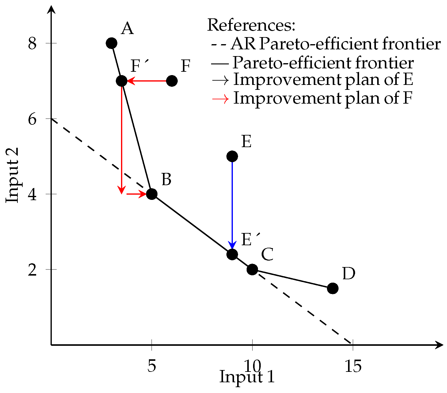
3.2. Numerical Example

In Section 3.2, we present a simple example that illustrates the practical implementation of our model, highlighting its ability to generate closest targets under weight restrictions in an intuitive manner.

Table 1. Numerical example.

DMU	X1	X2	Y1	${\mathit{\rho }}_{\mathit{j}}^{*}$	${\mathit{\varphi }}_{\mathit{j}}^{*}$	Condition
A	3	8	10	0	6	Pareto-Efficient
B	5	4	10	0	0	AR Pareto-Efficient
C	10	2	10	0	0	AR Pareto-Efficient
D	14	1.5	10	0	4.5	Pareto-Efficient
E	9	5	10	2.6	0	Non Pareto-Efficient
F	6	7	10	2.5	4.5	Non Pareto-Efficient

presents a set of DMUs that employ two inputs to generate a constant output. The DEA-VRS analysis indicates that DMUs A, B, C, and D are Pareto-efficient. In contrast, DMUs E and F are inefficient.

Below we incorporate the following information about the relative importance between inputs.

$$\begin{array}{cc}\hfill 5/3& \le {\displaystyle \frac{v_1}{v_2}}\le 4\hfill \end{array}$$

(8)

Once the weight restrictions are incorporated, some DMUs no longer lie on the modified efficient frontier, while others, such as DMUs B and C, remain AR Pareto-efficient—see Figure 1. When conditions on the weights are applied, part of the original efficient frontier is no longer valid, causing some previously efficient units, such as DMU A and DMU D, to become inefficient. In fact, DMU A, after the incorporation of Constraint (8), becomes inefficient and requires additional guidelines or efforts to reach the AR-efficient frontier. In this case, its target coordinates are those of DMU B. A similar situation occurs with DMU D. Note that, as [40] states, the standard second stage applied to radial models with weight restrictions may result in benchmarks with negative slack values for some inputs. It is also worth noting that, as with the conventional second stage used with the radial models, Model (3) may produce some negative target values. The authors of [40] propose a corrected procedure for the conventional second stage that ensures the non-negativity of the variables (see that paper for details). Therefore, an alternative is to use non-radial models and absolute values. To achieve this, we have applied our Model (6), which offers us the same targets for these two inefficient AR DMUs—see

Table 2. Improvement plans of Model (6).

DMU	Targets		% of Changes
	${\mathit{X}}_{\mathbf{1}}$	${\mathit{X}}_{\mathbf{2}}$	${\mathit{X}}_{\mathbf{1}}$	${\mathit{X}}_{\mathbf{2}}$
A	5	4	66.66	50
D	10	2	28.57	0
E	9	2.4	0	52
F	6	3.6	16.66	42.58

. In the case of Unit E, the shortest distance to the unrestricted frontier coincides with that obtained after adding WR, resulting in the target, point E’, with its peers in this case being DMUs B and C—Improvement plan are highlighted with blue arrows in Figure 1. Now, consider DMU F. Model (6), would provide us with a reference target, which in this case would be the projection F’ on the original efficient frontier. This reference target represents the coordinates from which we aim to deviate as little as possible, with the objective of obtaining improvement plans that require the least overall effort, which would lead us to the coordinates of DMU B, as it is the closest to point F’ on the AR efficient frontier—Figure 1 shows the improvement plan marked with red arrows.

4. Empirical Example

This section provides an empirical illustration of the proposed methodology. Specifically, we apply the proposed models to a real dataset that evaluates the performance of tourist localities in the province of Córdoba, Argentina, for the year 2022 (the most recent available data).

Córdoba is a province situated in the central of Argentina. It covers an area of 165,321 km² and has a population of over 4 million. The province features diverse landscapes, including mountains, rivers, lakes, plains, and green wooded areas. Córdoba’s main economic sectors are tourism, agriculture, and industry. These activities are of particular interest to stakeholders, making it essential to measure their performance. Such data are crucial for informed decision making, benefiting private sector operations and those responsible for formulating public policies—groups that currently lack this type of information.

In terms of tourism, Córdoba is the second most important tourist destination in Argentina, after the Atlantic coast of the province of Buenos Aires. It is mainly a national destination. More than 90% of visitors are Argentines, mainly families and middle-class people. The region of Córdoba stands out for its tourist activity, the number of visitors and its accommodation capacity, with an average of around 1 million beds available per year [41].

4.1. Selection of Variables and Data

In order to select the variables, we consider the information provided by the Tourist Information System of Argentina (https://datos.yvera.gob.ar/) and the National Institute of Statistics and Censuses (https://censo.gob.ar/) both accessed on 1 July 2024. The variables are described below, categorized as either inputs or outputs.

Inputs

• PL: Number of hotel beds available.
• EN: Number of firms directly or indirectly involved in tourism. Includes, for example, hotels and similar establishments providing collective accommodation, restaurants, amusement parks, and other tourist attractions.
• EAP: Number of economically active people living in the locality. This variable includes people over 18 years of age who are employed or actively seeking employment.

Outputs

• LP: Number of passengers arriving at each location. To reflect the impact on nearby localities (a decreasing proportion of passengers is assigned to locations within a radius of 15 km).
• AP: Number of passengers arriving on domestic and international flights corrected by the time of arrival at the location. Each airport influences a radius of 300 km.

According to the DEA framework, inputs represent the resources employed to obtain the outputs. In this context, PL and EN represent the capacity to accommodate tourism in a locality, while EAP represents the human resources potentially available for the activity. In case of outputs, both measure the number of passengers visiting each locality according to the classification, differentiated by their mode of transport.

Table 3. Normalized data.

Code	Locality	Inputs			Outputs
		PL	EN	EPA	LP	AT
AGO	Agua de Oro	0.318	0.154	0.089	0.059	0.512
AGR	Alta Gracia	0.716	1.155	1.631	0.666	1.667
ALM	Almafuerte	0.184	0.319	0.345	0.525	0.433
ALP	Arroyo Los Patos	0.204	0.165	0.035	0.460	0.303
ANI	Anisacate	0.201	0.187	0.230	0.276	0.568
ARY	Arroyito	0.200	0.242	0.770	0.345	0.418
BAL	Balnearia	0.041	0.066	0.187	0.057	0.239
BMA	Bialet Massé	0.367	0.418	0.259	0.975	0.583
CAB	Cabalango	0.122	0.330	0.016	0.935	0.546
CBA	Córdoba	8.494	25.998	40.547	18.942	22.736
CBL	Cuesta Blanca	0.184	0.253	0.017	0.842	0.534
CCA	Colonia Caroya	0.215	0.418	0.692	0.192	1.043
CCU	La Cumbrecita	0.402	0.330	0.020	0.224	0.280
CEJ	Cruz del Eje	0.106	0.176	0.795	0.174	0.318
CGR	Casa Grande	0.172	0.154	0.037	0.429	0.523
CMO	Capilla del Monte	2.252	1.815	0.337	0.748	0.437
CQN	Cosquín	1.863	1.199	0.659	1.114	0.546
CUA	Río Cuarto	1.413	2.716	4.800	4.319	1.022
EMB	Embalse	0.365	0.594	0.260	0.494	0.407
FRA	San Francisco	0.569	0.561	1.898	1.086	0.845
HGR	Huerta Grande	2.238	0.583	0.207	0.695	0.516
JES	Jesús María	0.193	0.583	1.009	0.302	1.039
LBO	Villa La Bolsa	0.104	0.176	0.039	0.365	0.549
LCA	Las Calles	0.092	0.099	0.018	0.195	0.269
LCO	Los Cocos	0.508	0.253	0.037	0.467	0.448
LCU	La Cumbre	1.331	0.704	0.189	0.498	0.471
LDR	Villa Dolores	0.412	0.572	0.862	0.768	0.131
LFA	La Falda	4.688	1.595	0.439	1.512	0.538
LGR	La Granja	0.210	0.154	0.133	0.087	0.489
LHO	Los Hornillos	0.168	0.187	0.048	0.313	0.243
LPO	La Población	0.048	0.044	0.020	0.079	0.123
LRA	Las Rabonas	0.245	0.198	0.024	0.245	0.258
LRE	Los Reartes	0.550	0.561	0.082	0.261	0.411
LSE	La Serranita	0.230	0.165	0.016	0.162	0.531
LVA	Las Varillas	0.107	0.154	0.515	0.274	0.250
MCL	Mina Clavero	5.160	3.046	0.297	1.749	2.509
MIR	Miramar	0.843	0.792	0.076	0.562	0.202
MSJ	Mayu Sumaj	0.084	0.187	0.076	0.893	0.549
NON	Nono	1.346	1.023	0.054	0.675	0.291
PAN	Panaholma	0.032	0.066	0.006	0.223	0.228
PGR	Potrero de Garay	0.542	0.429	0.061	0.351	0.471
RCE	Río Ceballos	0.846	0.693	0.741	0.221	0.564
RCR	Río Tercero	0.230	0.429	1.398	0.908	0.949
SAA	San Antonio de Arredondo	0.362	0.363	0.159	0.848	0.546
SAL	Salsipuedes	0.253	0.286	0.440	0.068	0.557
SJD	San José de la Dormida	0.071	0.077	0.136	0.170	0.411
SLO	San Lorenzo	0.165	0.165	0.055	0.346	0.273
SMS	San Marcos Sierra	0.594	0.660	0.077	0.163	0.318
SRC	Santa Rosa de Calamuchita	3.560	3.057	0.511	1.547	2.015
SRO	San Roque	0.037	0.110	0.065	0.623	0.602
TAN	Tanti	1.003	0.748	0.289	0.693	0.542
THU	Tala Huasi	0.124	0.132	0.005	0.689	0.512
UNQ	Unquillo	0.075	0.396	0.700	0.201	0.557
VAL	Villa Allende	0.096	0.594	1.016	0.359	0.583
VCA	Villa Ciudad de América	0.279	0.176	0.031	0.275	0.497
VCB	Villa Cura Brochero	1.565	1.199	0.211	0.762	0.841
VCP	Villa Carlos Paz	13.407	5.620	1.870	7.189	7.198
VDI	Villa del Dique	0.619	0.528	0.137	0.500	0.273
VGB	Villa General Belgrano	3.176	2.013	0.313	1.508	2.382
VGI	Villa Giardino	1.688	0.693	0.194	1.179	0.504
VHE	Valle Hermoso	1.211	0.506	0.190	1.358	0.549
VIC	Villa Río Icho Cruz	0.397	0.275	0.075	0.988	0.546
VLR	Villa Cdad Pque Los Reartes	0.216	0.297	0.074	0.906	0.411
VMA	Villa María	0.993	0.638	2.652	2.048	1.451
VPS	Villa Parque Siquimán	0.190	0.231	0.093	0.905	0.594
VRO	Villa de las Rosas	0.081	0.165	0.154	0.327	0.202
VRU	Villa Rumipal	0.503	0.429	0.108	0.317	0.314
VSC	Villa Santa Cruz del Lago	0.261	0.154	0.096	0.859	0.564
VTO	Villa del Totoral	0.203	0.209	0.289	0.210	0.504
VYA	Villa Yacanto	0.275	0.341	0.090	0.296	0.265

shows the data for 70 localities in the province of Córdoba. The data have been normalized by the average: 14,375 places, 91 companies, 24,244 economically active people, 62,937 visitors by land, and 9095 by air.

4.2. DEA Analysis

Firstly, we extract relevant information from the dataset. Applying the additive DEA model proposed in [37], 19 Pareto-efficient units are obtained out of 70, while 51 are classified as inefficient. The efficient DMUs are CAB, CBA, CCA, CUA, JES, LPO, MCL, MSJ, PAN, RCR, SJD, SRO, THU, VCP, VGB, VHE, VIC, VMA, and VSC.

To obtain the closest target, which we will later use as reference targets to provide improvement plans, we use Model (3). The results are presented in

Table 4. Closest target and global efforts.

Code	${\mathit{p}}_{\mathit{j}}^{*}$	Code	${\mathit{p}}_{\mathit{j}}^{*}$	Code	${\mathit{p}}_{\mathit{j}}^{*}$	Code	${\mathit{p}}_{\mathit{j}}^{*}$
AGO	0.704	CQN	1.227	LRE	1.022	UNQ	1.068
AGR	0.146	EMB	0.794	LSE	0.600	VAL	1.224
ALM	0.414	FRA	0.606	LVA	0.647	VCA	0.574
ALP	0.210	HGR	1.753	MIR	1.146	VCB	0.828
ANI	0.512	LBO	0.358	NON	1.524	VDI	0.941
ARY	0.961	LCA	0.152	PGR	0.719	VGI	0.877
BAL	0.328	LCO	0.608	RCE	1.083	VLR	0.203
BMA	0.164	LCU	1.178	SAA	0.215	VPS	0.021
CBL	0.048	LDR	0.988	SAL	0.736	VRO	0.316
CCU	0.674	LFA	3.352	SLO	0.229	VRU	0.904
CEJ	0.866	LGR	0.512	SMS	1.163	VTO	0.634
CGR	0.312	LHO	0.279	SRC	1.156	VYA	0.566
CMO	1.967	LRA	0.341	TAN	0.781

. The value $p_j^{*}$ represents the minimum overall effort required to reach the original (i.e., without WR) Pareto-efficient frontier. In particular, we could argue that VPS, CBL, and AGR localities would be the ones that would require the least effort to achieve efficiency levels in the Pareto sense. On the other hand, LFA, CMO, and HGR would be the localities that would require the most effort to achieve optimal efficiency levels.

4.3. Weight Restrictions

The principal objective of this study is to ensure that the processes of benchmarking and target setting align with the widely accepted views of experts regarding the significance of both the resources (inputs) utilized by localities and their results (outputs).

To determine the relative importance of the variables under consideration, the opinions of 11 experts were sought on each set of inputs and outputs. The panel of experts consisted of five civil servants from the localities’ tourism departments, four CEOs of tourism companies, and two tourism consultants.

The weightings assigned to each variable were determined using the Analytic Hierarchy Process (AHP). This methodology was applied to determine weights in DEA problems by authors such as [42,43,44]. AHP is a discrete multi-criteria decision making method that was developed in 1980 by [45]. This method involves decomposing a problem into a hierarchical structure and making pairwise comparisons of the relative importance of the elements within the model. This approach allows the determination of the contribution of each element to the final decision through the synthesis of priorities at each level, expressed in the form of weights. The process can be summarized in the following steps.

Step 1: Structure the decision problem into hierarchical levels. This hierarchy should clearly identify the fundamental elements of the problem, organize them into levels, and represent the objective, criteria, and alternatives.

Step 2: Perform pairwise comparisons between the decision elements at each hierarchical level. This involves a comparison of the criteria with respect to each other, as well as a comparison of the alternatives with respect to each criterion. The authors of [45] suggest the use of the Fundamental Scale to facilitate these comparisons. Each value on this scale reflects a verbal judgment by the decision maker regarding the preference of one element over another.

Step 3: Apply the eigenvalue method to determine the relative weights or priorities of the decision elements. A weight vector is obtained as $w_i^k$ = $(w_1^k,...,w_m^k)$, with ${\sum }_{i=1}^m{w}_i^k=1$ for both cases, inputs and outputs, where k is associated with the expert.

Step 4: Assess the consistency of the decision maker’s judgments by calculating the Consistency Ratio. If this ratio exceeds a predefined threshold, it indicates the need to revise the judgments to improve consistency.

Step 5: Perform an overall evaluation of each alternative, summarizing the results in a vector of weights.

Table 5. AHP weights and consistency judgments.

	${\mathit{w}}_{\mathit{PL}}$	${\mathit{w}}_{\mathit{EN}}$	${\mathit{w}}_{\mathit{EPA}}$	${\mathit{w}}_{\mathit{LP}}$	${\mathit{w}}_{\mathit{AP}}$
Exp1	0.6479	0.2299	0.1222	0.6667	0.3333
Exp2	0.3338	0.5247	0.1416	0.3472	0.6528
Exp3	0.3601	0.1279	0.5119	0.8333	0.1667
Exp4	0.7028	0.1822	0.1149	0.3333	0.6667
Exp5	0.4000	0.3667	0.2333	0.6667	0.3333
Exp6	0.2000	0.6000	0.2000	0.8571	0.1429
Exp7	0.3113	0.6227	0.0660	0.8333	0.1667
Exp8	0.3591	0.5644	0.0765	0.8333	0.1667
Exp9	0.6584	0.2618	0.0798	0.8571	0.1429
Exp10	0.4577	0.4160	0.1263	0.8750	0.1250
Exp11	0.4484	0.2884	0.2632	0.8333	0.1667

shows the weight of each variable and the result of consistency evaluation. From the consistency analysis, we observe that experts 5 and 11 did not demonstrate consistency in their evaluations, and were therefore excluded from the subsequent analysis.

The information provided for the expert can be used in different ways. In [46,47], AR-type 1 is proposed, which involves imposing restrictions on the upper bound (U) and lower bound (L) of the ratio of weights between two variables $L_{i{i}^{\prime }}\le v_i/v_{i^{\prime }}\le U_{i{i}^{\prime }}$, where $L_{i{i}^{\prime }}=mi{n}_k(w_i^k/w_{i^{\prime }}^k)$ and $U_{i{i}^{\prime }}=ma{x}_k(w_i^k/w_{i^{\prime }}^k)$ in the case of inputs and $L_{r{r}^{\prime }}\le w_r/w_{r^{\prime }}\le U_{r{r}^{\prime }}$ where $L_{r{r}^{\prime }}=mi{n}_k(w_r^k/w_{r^{\prime }}^k)$ and $U_{r{r}^{\prime }}=ma{x}_k(w_r^k/w_{r^{\prime }}^k)$ in the case of outputs, with k being the superscript associated with the experts involved. Specifically, the constraints in (9) represent the AR restrictions to be added to Model (6).

$$\begin{array}{cc}\hfill 0.3333& \le {\displaystyle \frac{v_{PL}}{v_{EN}}}\le 3.8568\hfill \\ \hfill 0.7035& \le {\displaystyle \frac{v_{PL}}{v_{EPA}}}\le 8.2488\hfill \\ \hfill 0.2499& \le {\displaystyle \frac{v_{EN}}{v_{EPA}}}\le 9.4391\hfill \\ \hfill 0.5& \le {\displaystyle \frac{u_{LP}}{u_{AT}}}\le 7\hfill \end{array}$$

(9)

In (9), a significant variability in the ratios of DEA weights can be observed. Consequently, in many cases, these constraints have minimal impact on the overall flexibility of the weights. This is due to the dispersion of expert opinion. For instance, the PL input has a range of variation of 0.5028, with a maximum value of 0.7028 and a minimum of 0.2.

Restrictions (9) are incorporated into the analysis and Model (6) is resolved. Ten Pareto-efficient DMUs are identified: CAB, CBA, CUA, MSJ, LPO, PAN, SRO, THU, VCP, and VMA.

Table 6. Inefficient DMUs and their benchmark.

Inefficient DMU	CAB	CBA	CUA	MSJ	LPO	PAN	SRO	THU	VCP	VMA
AGO	0	0	0	0	0	0.469	0.531	0	0	0
AGR	0	0.031	0	0.89	0	0	0	0	0.024	0.055
ALM	0	0.007	0	0	0	0	0.993	0	0	0
ALP	0.174	0	0	0.108	0	0	0.339	0.379	0	0
ANI	0	0.002	0	0	0	0	0.972	0	0	0.026
ARY	0	0	0	0	0	0	0.925	0	0.008	0.067
BAL	0	0	0	0	0.032	0.968	0	0	0	0
BMA	0.333	0	0.037	0.614	0	0	0	0	0.016	0
CBL	0.605	0	0	0.036	0	0	0.038	0.321	0	0
CCA	0	0	0	0	0.209	0.791	0	0	0	0
CCU	0	0	0	0	0	0.86	0.14	0	0	0
CEJ	0	0	0	0	0.334	0.666	0	0	0	0
CGR	0.133	0	0	0.083	0	0	0.408	0.376	0	0
CMO	0.933	0	0.067	0	0	0	0	0	0	0
CQN	0.854	0	0.127	0	0	0	0	0	0.019	0
EMB	0	0	0	0	0	0	0.919	0	0.02	0.061
FRA	0	0.008	0	0	0	0	0.501	0	0	0.491
HGR	0.948	0	0.032	0	0	0	0	0	0.02	0
JES	0	0.018	0	0	0	0	0.98	0	0	0.002
LBO	0.28	0	0	0	0	0	0.52	0.2	0	0
LCA	0	0	0	0	0	0.89	0.11	0	0	0
LCO	0.573	0	0	0	0	0	0.427	0	0	0
LCU	0	0.002	0	0	0	0	0.982	0	0	0.016
LDR	0.899	0	0.101	0	0	0	0	0	0	0
LFA	0.912	0	0.088	0	0	0	0	0	0	0
LGR	0	0	0	0	0	0.666	0.334	0	0	0
LHO	0	0	0	0	0	0.685	0.315	0	0	0
LRA	0	0	0	0	0	0.91	0.09	0	0	0
LRE	0	0	0	0	0	0.51	0.49	0	0	0
LSE	0.083	0	0	0	0	0	0.163	0.754	0	0
LVA	0	0	0	0	0	0.888	0.013	0.099	0	0
MCL	0.849	0	0	0	0	0	0	0	0.151	0
MIR	0	0	0	0	0	0.494	0.088	0.418	0	0
NON	0	0	0	0.517	0	0	0.213	0.27	0	0
PGR	0	0	0	0	0	0.35	0.65	0	0	0
RCE	0	0	0	0	0.009	0.991	0	0	0	0
RCR	0	0.01	0	0	0	0	0.877	0	0	0.113
SAA	0.274	0	0.014	0.693	0	0	0	0	0.019	0
SAL	0	0	0	0	0	0.614	0.386	0	0	0
SJD	0	0	0	0	0.367	0.633	0	0	0	0
SLO	0	0	0	0	0	0.583	0.417	0	0	0
SMS	0	0	0	0	0.181	0.819	0	0	0	0
SRC	0	0	0	0	0	0	0.759	0	0.229	0.012
TAN	0	0	0.021	0.916	0	0	0	0	0.063	0
UNQ	0	0.004	0	0	0	0	0.995	0	0	0.001
VAL	0	0.007	0	0	0	0	0.992	0	0	0.001
VCA	0.251	0	0	0.033	0	0	0.345	0.371	0	0
VCB	0	0	0	0	0	0	0.886	0	0.114	0
VDI	0.189	0	0	0.771	0	0	0	0	0.04	0
VGB	0.84	0	0	0	0	0	0	0	0.16	0
VGI	0.951	0	0.029	0	0	0	0	0	0.02	0
VHE	0.951	0	0.029	0	0	0	0	0	0.02	0
VIC	0.279	0	0	0.712	0	0	0	0	0.009	0
VLR	0.416	0	0.001	0.574	0	0	0	0	0.009	0
VPS	0	0	0	0.831	0	0	0.159	0	0.008	0.002
VRO	0	0	0	0	0	0.831	0.027	0.142	0	0
VRU	0	0	0	0	0	0.369	0.631	0	0	0
VSC	0	0	0	0.525	0	0	0.461	0	0.014	0
VTO	0	0.004	0	0	0	0	0.97	0	0	0.026
VYA	0	0	0	0	0	0.502	0.498	0	0	0
Times as referents	21	10	11	14	6	21	38	10	19	13

presents the inefficient DMUs along with their corresponding benchmarks, represented by the variable ${\lambda }_j^{*}$. ${\lambda }_j^{*}$ is defined as the intensity with which an efficient DMU contributes to the activities of an inefficient DMU. A value of zero in ${\lambda }_j^{*}$ indicates that the DMU is not being benchmarked, whereas a value greater than zero signifies that the DMU acts as a peer and is benchmarked at the specified intensity. For example, AGO should project onto the best practice frontier by setting its target as a combination of 0.469 from PAN and 0.531 from SRO.

SRO, PAN, CAB, and VCP are the most frequently selected benchmarks. It was observed that all inefficient DMUs selected at least one of these four as a benchmark. Notably, SRO was selected as benchmark for 38 DMUs, out of a total of 60. In contrast, LPO was selected as a referent only six times. CAB, MSJ, SRO, and THU are localities with fewer resources yet they attract a large number of visitors. They serve as benchmarks for many other localities facing similar circumstances. CBA is the largest locality in the province and does not have a comparable peer. Therefore, it is reasonable for CBA to be an efficient locality without serving as a benchmark for other localities or, at least, with limited intensity. In contrast, the cities of CUA, VCP, and VMA are smaller in size compared to Cordoba; however, they have the necessary infrastructure to provide outputs. Consequently, it is not surprising that they serve as reference points for localities such as FRA, MCL, SRC, and others.

Regarding targets,

Table 7. Inefficient DMUs and their targets.

Inefficient DMU	Inputs			Outputs		Inefficient DMU	Inputs			Outputs
	PL	EN	EPA	LT	AT		PL	EN	EPA	LT	AT
AGO						AGR
Data	4571	14	2158	3713	4657	Data	10293	105	39542	41916	15161
Targets	489	8	897	27378	3874	Targets	10293	105	37215	105419	13242
% Change	−89.2%	−42.0%	−58.1%	638.9%	−16.7%	% Change	0.0%	0.0%	−5.9%	151.4%	−12.7%
ALM						ALP
Data	2645	29	8364	33042	3938	Data	2933	15	849	28951	2756
Targets	1409	27	8728	47643	6939	Targets	1294	15	849	46070	5020
% Change	−46.5%	−6.4%	4.2%	44.2%	76.0%	% Change	−56.0%	0.0%	0.0%	59.0%	82.4%
ANI						ARY
Data	2889	17	5576	17371	5166	Data	2875	22	18668	21713	3802
Targets	1179	17	5576	44371	6166	Targets	2875	17	6134	48336	6439
% Change	−59.3%	0.0%	0.0%	155.7%	19.3%	% Change	0.0%	−23.0%	−67.2%	122.8%	69.1%
BAL						BMA
Data	589	6	4534	3587	2174	Data	5276	38	6279	61364	5302
Targets	460	6	145	13720	2046	Targets	5276	38	6279	71622	6148
% Change	−21.2%	0%	−96.6%	283.3%	−6.1%	% Change	0.0%	0.0%	0.0%	16.7%	16.0%
CBL						CCA
Data	2645	23	412	52993	4857	Data	3091	38	16777	12084	9486
Targets	1696	23	412	52993	4884	Targets	503	6	218	12084	1874
% Change	−35.8%	0.0%	0.0%	0.0%	0.5%	% Change	−83.7%	−85.3%	−98.7%	0.0%	−80.2%
CCU						CEJ
Data	5779	30	485	14098	2547	Data	1524	16	19274	10951	2892
Targets	460	7	339	17559	2547	Targets	532	5	267	10951	1755
% Change	−91.9%	−78.1%	−29.5%	24.4%	0.0%	% Change	−65.1%	−66.7%	−98.7%	0.0%	−39.2%
CGR						CMO
Data	2473	14	897	27000	4757	Data	32373	165	8170	47077	3975
Targets	1222	14	897	44811	5057	Targets	2990	45	8170	73070	5248
% Change	−50.8%	0.0%	0.0%	66.1%	6.3%	% Change	−90.7%	−73.0%	0.0%	55.4%	32.1%
CQN						EMB
Data	26781	109	15977	70112	4966	Data	5247	54	6303	31091	3702
Targets	7619	67	15977	93147	6621	Targets	5247	23	6303	53056	7158
% Change	−71.6%	−39.0%	0.0%	32.8%	33.5%	% Change	0.0%	−57.3%	0.0%	70.6%	93.1%
FRA						HGR
Data	8179	51	46015	68350	7685	Data	32171	53	5019	43741	4693
Targets	8179	51	39639	91825	10750	Targets	6224	47	5019	73636	6330
% Change	0.0%	0.0%	−13.8%	34.3%	39.9%	% Change	−80.6%	−11.9%	0.0%	68.4%	35.0%
JES						LBO
Data	2774	53	24462	19007	9450	Data	1495	16	946	22972	4993
Targets	2774	53	19589	60420	9159	Targets	1121	16	946	45566	5166
% Change	0.0%	0.0%	−19.9%	217.8%	−3.1%	% Change	−24.7%	0.0%	0.0%	98.2%	3.4%
LCA						LCO
Data	1323	9	436	12273	2447	Data	7303	23	897	29392	4075
Targets	460	6	291	16804	2447	Targets	1222	21	897	50475	5175
% Change	−64.9%	−28.4%	−32.3%	37.1%	0.0%	% Change	−83.2%	−6.7%	0.0%	71.6%	27.0%
LCU						LDR
Data	19133	64	4582	31343	4284	Data	5923	52	20898	48336	1191
Targets	992	16	4582	43049	6003	Targets	3637	52	12146	80433	5402
% Change	−94.8%	−75.7%	0.0%	37.2%	40.2%	% Change	−38.6%	0.0%	−41.9%	66.4%	354.3%
LFA						LGR
Data	67390	145	10643	95161	4893	Data	3019	14	3224	5476	4447
Targets	3393	49	10643	77664	5348	Targets	474	7	630	22469	3211
% Change	−95.0%	−66.1%	0.0%	−18.4%	9.2%	% Change	−84.1%	−47.6%	−80.8%	311.1%	−27.9%
LHO						LRA
Data	2415	17	1164	19699	2210	Data	3522	18	582	15420	2347
Targets	474	7	582	21965	3147	Targets	460	6	267	16238	2374
% Change	−80.2%	−57.3%	−49.2%	11.7%	42.4%	% Change	−86.8%	−64.7%	−54.4%	5.6%	1.4%
LRE						LSE
Data	7906	51	1988	16427	3738	Data	3306	15	388	10196	4829
Targets	489	8	849	26371	3738	Targets	1567	13	388	43993	4811
% Change	−93.8%	−84.4%	−57.6%	60.8%	0.0%	% Change	−52.6%	−12.2%	0.0%	332.4%	−0.2%
LVA						MCL
Data	1538	14	12486	17245	2274	Data	74175	277	7200	110077	22819
Targets	589	7	170	17245	2374	Targets	30676	103	7200	118447	14125
% Change	−61.8%	−52.5%	−98.7%	0.0%	4.3%	% Change	−58.6%	−62.9%	0.0%	7.6%	−38.1%
MIR						NON
Data	12118	72	1843	35371	1837	Data	19349	93	1309	42482	2647
Targets	1021	9	267	28510	3447	Targets	1222	14	1309	49154	5002
% Change	−91.6%	−87.7%	−85.8%	−19.5%	88.0%	% Change	−93.7%	−84.8%	0.0%	15.6%	88.8%
PGR						RCE
Data	7791	39	1479	22091	4284	Data	12161	63	17965	13909	5130
Targets	503	9	1067	30399	4284	Targets	460	6	145	13909	2065
% Change	−93.5%	−78.0%	−27.2%	37.7%	0.0%	% Change	−96.2%	− 90.5%	−99.2%	0.0%	−59.8%
RCR						SAA
Data	3306	39	33893	57147	8631	Data	5204	33	3855	53371	4966
Targets	3306	39	18498	60923	8358	Targets	5204	33	3855	67343	6176
% Change	0.0%	0.0%	−45.4%	6.6%	−3.2%	% Change	0.0%	0.0%	0.0%	26.1%	24.5%
SAL						SJD
Data	3637	26	10667	4280	5066	Data	1021	7	3297	10699	3738
Targets	489	8	703	23727	3383	Targets	546	5	267	10699	1719
% Change	−86.7%	−71.0%	−93.5%	458.6%	−33.2%	% Change	−47.1%	−24.8%	−91.9%	0.0%	−53.9%
SLO						SMS
Data	2372	15	1333	21776	2483	Data	8539	60	1867	10259	2892
Targets	489	8	727	24545	3492	Targets	503	6	194	12399	1901
% Change	−79.5%	−48.9%	−44.9%	12.5%	40.6%	% Change	−94.2%	−90.6%	−89.1%	20.3%	−34.2%
SRC						TAN
Data	51175	278	12389	97364	18326	Data	14418	68	7007	43615	4929
Targets	44649	125	12389	134874	19290	Targets	13599	53	7007	85657	8868
% Change	−12.8%	−55.0%	0.0%	38.5%	5.2%	% Change	−5.7%	−22.3%	0.0%	96.4%	80.0%
UNQ						VAL
Data	1078	36	16971	12650	5066	Data	1380	54	24632	22594	5302
Targets	1078	21	6013	44434	6376	Targets	1380	26	8413	47266	6867
% Change	0.0%	−42.8%	−64.6%	251.7%	26.0%	% Change	0.0%	−51.2%	−65.9%	109.1%	29.6%
VCA						VCB
Data	4011	16	752	17308	4520	Data	22497	109	5115	47958	7649
Targets	1323	16	752	46259	5030	Targets	22497	67	6570	86475	12333
% Change	−67.0%	0.0%	0.0%	167.3%	11.2%	% Change	0.0%	−38.3%	28.3%	80.2%	61.2%
VDI						VGB
Data	8898	48	3321	31469	2483	Data	45655	183	7588	94909	21664
Targets	8898	39	3321	72440	7385	Targets	32344	107	7588	121909	14652
% Change	0.0%	−18.6%	0.0%	130.3%	197.7%	% Change	−29.2%	−41.5%	0.0%	28.4%	−32.4%
VGI						VHE
Data	24265	63	4703	74203	4584	Data	17408	46	4606	85468	4993
Targets	6181	46	4703	73070	6321	Targets	6181	46	4606	72944	6321
% Change	−74.5%	−26.7%	0.0%	−1.5%	37.8%	% Change	−64.5%	0.0%	0.0%	−14.7%	26.5%
VIC						VLR
Data	5707	25	1818	62182	4966	Data	3105	27	1794	57021	3738
Targets	3062	25	1818	60420	5521	Targets	3105	27	1794	61049	5502
% Change	−46.5%	0.0%	0.0%	−2.8%	11.3%	% Change	0.0%	0.0%	0.0%	7.1%	47.3%
VPS						VRO
Data	2731	21	2255	56958	5402	Data	1164	15	3734	20580	1837
Targets	2731	20	2255	56958	5593	Targets	647	7	170	18881	2528
% Change	0.0%	−4.2%	0.0%	0.0%	3.5%	% Change	−44.6%	−53.6%	−95.2%	−8.3%	37.9%
VRU						VSC
Data	7231	39	2618	19951	2856	Data	3752	14	2327	54063	5130
Targets	503	9	1042	29958	4220	Targets	3637	21	2327	54063	6075
% Change	−93.1%	−78.1%	−60.2%	50.2%	47.8%	% Change	−3.3%	48.8%	0.0%	0.0%	18.5%
VTO						VYA
Data	2918	19	7007	13217	4584	Data	3953	31	2182	18629	2410
Targets	1294	19	6449	45378	6339	Targets	489	8	849	26559	3765
% Change	−55.7%	0.0%	−7.7%	244.1%	38.1%	% Change	−87.5%	−74.2%	−60.8%	42.4%	56.0%

presents the observed data alongside the set targets, including both the projected values and the percentage improvements. The latter are calculated as the difference between the observed values in each dimension and their respective projections, adjusted for the observed value.

It can be observed that the improvement plans proposed for the BMA, FRA, RCR, SAA, VLR, VPS, and VSC localities are very similar to their performance values, so the efforts required to achieve the targets are minimal. Conversely, ARY, EMB, JES, TAN, UNQ, VAL, VCB, and VDI exhibit significant deviations from their actual values, requiring more substantial changes to achieve efficiency. Finally, there are two cases, VCP and VMA, in which the AR target are very similar to the reference target obtained with (3).

A significant proportion of inefficient localities require only minimal efforts to achieve optimal levels of efficiency in certain variables. When analyzing each variable individually, and considering an effort below 10% as both acceptable and easily achievable, it is found that 26% of inefficient localities need minimal changes in the input PL, 35% require less than a 10% improvement in input EN, 51.6% in input EPA, 25% in output LP, and 26.6% in output AT. A notable exception is VPS, where the required adjustments across all variables are below 7.73%.

Regarding the most extreme adjustments, the highest efforts are found in the outputs. Localities such as ALG, SAL, and VTO should implement policies designed to attract more visitors. This trend, however, is not observed in the inputs.

Model (6) assumes that slack variables can take values within the real set. In certain cases, changes may be considered counterintuitive, such as an increase in input or a decrease in output. The former group includes the locations ALM, VCG, and VSC, while the latter includes examples such as VIC, VRO, VHE, SMS, SJD, RCE, LSE, MIR, RCR, SAL, and VGI. These adjustments suggest that the model allows flexibility in resource allocation, even when such changes may seem unconventional.

Several localities deserve special attention. VGB, which is widely recognized in Argentina for its infrastructure and high level of commitment to event organization, is efficient in the Pareto sense. However, when expert opinions are incorporated, it becomes inefficient, as experts perceive it as unbalanced. A similar, though less pronounced, case is observed in the localities of CQN and MCL. On the other hand, localities like LCU and NON, which are particularly known for their natural beauty or gastronomy, show relatively minimal changes needed to achieve the AR frontier.

Localities such as MCL and NON are well known and considered key tourist destinations, although they require substantial resources relative to the number of visitors they attract. These localities, together with VCB, belong to the same tourist circuit and should collaborate on developing joint policy improvement plans to optimize their input–output relationship.

Finally, it should be noted that the most significant tourist routes in the province of Córdoba are Punilla, Calamuchita, and Traslasierra, all of which have at least one locality that serves as a benchmark for the inefficient ones.

From an empirical perspective, and with the aim of comparing our approach to previous methodologies in the literature, we contrast our study with that of [30]. However, it is important to highlight that [30] aligns with [31] as both approaches focus on identifying the closest efficient target within a production technology modified by external information. Nonetheless, our use case is more closely related to [30] where AR-I-type weight restrictions are incorporated under the VRS assumption.

Note that [30] aims to project onto the AR-efficient frontier under the closest target approach. Similarly, we employ the minimum distance to this frontier but with the added condition of deviating as little as possible from the original closest target without AR constraints.

Table 8. Selected inefficient DMUs and their benchmark according to the proposal by [30].

Inefficient DMU	CAB	CBA	CUA	MSJ	LPO	PAN	SRO	THU	VCP	VMA
BMA	0.333	0	0.037	0.614	0	0	0	0	0.017	0
CCA	0	0	0	0	0.209	0.791	0	0	0	0
CCU	0	0	0	0	0	0.86	0.14	0	0	0
CEJ	0	0	0	0	0.334	0.666	0	0	0	0
EMB	0.941	0	0.046	0	0	0	0	0	0.014	0
JES	0	0.018	0	0	0	0	0.98	0	0	0.002
LRA	0	0	0	0	0	0.92	0.08	0	0	0
LRE	0	0	0	0	0	0.51	0.49	0	0	0
MCL	0.849	0	0	0	0	0	0	0	0.151	0
RCE	0	0	0	0	0.009	0.991	0	0	0	0
RCR	0	0.01	0	0	0	0	0.877	0	0	0.113
SAA	0.274	0	0.014	0.693	0	0	0	0	0.019	0
VAL	0	0.007	0	0	0	0	0.993	0	0	0
VGB	0.84	0	0	0	0	0	0	0	0.16	0
VGI	0.948	0	0.028	0	0	0	0	0	0.024	0
VHE	0.951	0	0.029	0	0	0	0	0	0.02	0
VIC	0.279	0	0	0.712	0	0	0	0	0.009	0
VLR	0.416	0	0.002	0.574	0	0	0	0	0.009	0
VSC	0	0	0	0.525	0	0	0.461	0	0.014	0
VYA	0	0	0	0	0	0.842	0	0.158	0	0
Times as referents	15	5	12	12	14	27	24	12	15	9

present the inefficient DMUs alongside their corresponding benchmarks based on [30]. Comparing these results with our approach reveals several notable differences.

We obtained identical or nearly identical solutions in 21 cases, approximately 35% (BMA, CCA, CCU, CEJ, JES, LFA, LRA, LRE, MCL, PGR, RCE, RCR, SAA, SJD, VAL, VGB, VGI, VHE, VIC, VLR, and VSC).

We find that the referenced units are consistent across both models, with the most representative DMUs being PAN, SRO, VCP, and CBA. Finally, we observe that in our approach, inefficient DMUs are projected onto a larger number of reference units.

Considering the inefficient DMUs, we observe that the benchmarks identified by the two approaches are generally different. For example, for EMB, ref. [30] identifies CAB, CUA, and VCP as benchmarks, while Model (6) identifies SRO, VCP, and VMA. Empirically, our approach appears to provide a better solution, since EMB is close to SRO and both are located in the same valley. The case of VYA is different. In our model, the projection intensity is very similar for PAN and SRO. However, in [30], not only is one of the benchmarks different—with THU replacing SRO—but the projection intensity also varies. For example, the intensity of PAN is 0.842. LSE is similar to VYA, but in this case, the projections are more balanced with [30].

Regarding lambdas, we do not observe significant differences between the two approaches. Both offer alternative solutions to project onto the AR frontier. However, we follow a more conservative philosophy by striving to remain as close as possible to the original closest target.

5. Conclusions

Benchmarking within a DEA framework has emerged as a powerful tool for performance evaluation and improvement across diverse sectors such as banking, education, healthcare, and transportation. By identifying benchmarks on the efficient frontier, organizations can establish actionable improvement plans that provide clear guidelines for inefficient Decision Making Units (DMUs) to achieve operational efficiency. The concept of the closest target, initially developed by [27], identifies the point on the Pareto-efficient frontier that minimizes the distance to the DMU under evaluation—a notion that has been further refined by numerous authors [1,2,6,29,30,32,33,39].

An essential element in effective benchmarking is the careful selection of peers. It is important not only to compare a DMU against industry leaders but also to consider direct competitors that share similar operational characteristics. Recent contributions [8,28,39] have underscored the importance of incorporating desirable criteria for peer selection, thereby ensuring that benchmarks are both realistic and strategically relevant. Moreover, the incorporation of expert opinion and value judgments through weight restrictions (WRs) addresses the challenge of unrestricted weight flexibility inherent in traditional DEA models, aligning the analysis more closely with managerial insights and practical constraints.

Building on this foundation, our work introduces a novel model that integrates the determination of the closest target, the incorporation of value judgments via WRs, and the identification of an ideal “peer.” Our approach focuses on deriving input and output targets for DMU₀ that lie on the Pareto-efficient frontier of the modified technology (i.e., the original technology adjusted by input and output weight constraints). Furthermore, these targets are designed to be as close as possible to the reference target obtained in an initial, unrestricted analysis, thereby ensuring that the recommended improvement plan represents a minimal and effective deviation from the optimal scenario. Overall, our proposed approach is designed to strike a balance these two objectives: integrating expert knowledge into the benchmarking process while preserving the core principles of the standard DEA framework.

Next, we outline both the theoretical and practical contributions of our approach.

Theoretical contributions:

• We extend the closest target framework in Data Envelopment Analysis (DEA) by incorporating weight restrictions, ensuring that efficiency benchmarks align with expert-imposed constraints.
• Our model introduces a two-step target setting approach that minimizes deviations from the unrestricted closest target while ensuring compliance with weight-restricted efficiency conditions.
• We propose a novel methodological framework that enhances the interpretability of DEA results, particularly in constrained benchmarking scenarios, by preserving the original efficiency structure as much as possible.

Practical contributions:

• Our approach offers decision makers a more realistic and actionable benchmarking tool by integrating expert preferences, making it particularly valuable in sectors where managerial insights play a crucial role, such as tourism, healthcare, and banking.
• We demonstrate the applicability of our model through an empirical study of tourism localities in Córdoba, Argentina, providing a practical example of how weight-restricted DEA can inform resource allocation and policy decisions.
• By ensuring that improvement plans require minimal effort while adhering to imposed constraints, our model provides a structured methodology for strategic planning and performance enhancement across various industries.

While our proposed model makes significant strides in integrating expert opinions with closest-target benchmarking, several promising directions for future research remain. One potential extension involves adapting the model to dynamic environments where DMUs’ performances evolve over time, thereby providing insights into into the long-term sustainability of improvement strategies. Additionally, incorporating stochastic elements to account for data uncertainty in inputs and outputs could enhance the robustness and reliability of the benchmarking process. Another promising direction is exploring the integration of multiple layers of expert judgment, possibly using fuzzy weighting approaches, which could better capture the complexity of managerial decision making. Finally, conducting empirical validations across diverse sectors and emerging economies would be valuable in assessing the model’s generalizability and practical applicability.

References

1. Aparicio, J.; Lopez-Espin, J.J.; Martinez-Moreno, R.; Pastor, J.T. Benchmarking in Data Envelopment Analysis: An Approach Based on Genetic Algorithms and Parallel Programming. Adv. Oper. Res. 2014, 2014, 431749. [Google Scholar] [CrossRef]
2. Ruiz, J.L.; Sirvent, I. Common benchmarking and ranking of units with DEA. Omega 2016, 65, 1–9. [Google Scholar] [CrossRef]
3. Cook, W.D.; Ruiz, J.L.; Sirvent, I.; Zhu, J. Within-group common benchmarking using DEA. Eur. J. Oper. Res. 2017, 256, 901–910. [Google Scholar] [CrossRef]
4. An, Q.; Tao, X.; Dai, B.; Xiong, B. Bounded-change target-setting approach: Selection of a realistic benchmarking path. J. Oper. Res. Soc. 2021, 72, 663–677. [Google Scholar] [CrossRef]
5. Lozano, S.; Soltani, N. A modified discrete Raiffa approach for efficiency assessment and target setting. Ann. Oper. Res. 2020, 292, 71–95. [Google Scholar] [CrossRef]
6. Ruiz, J.L.; Sirvent, I. Performance evaluation through DEA benchmarking adjusted to goals. Omega 2019, 87, 150–157. [Google Scholar] [CrossRef]
7. Aparicio, J.; Monge, J.F.; Ramón, N. A new measure of technical efficiency in data envelopment analysis based on the maximization of hypervolumes: Benchmarking, properties and computational aspects. Eur. J. Oper. Res. 2021, 293, 263–275. [Google Scholar] [CrossRef]
8. Borrás, F.; Ruiz, J.L.; Sirvent, I. Planning improvements through data envelopment analysis (DEA) benchmarking based on a selection of peers. Socio-Econ. Plan. Sci. 2024, 95, 102020. [Google Scholar] [CrossRef]
9. Zofio, J.L.; Aparicio, J.; Barbero, J.; Zabala-Iturriagagoitia, J.M. Benchmarking performance through efficiency analysis trees: Improvement strategies for Colombian higher education institutions. Socio-Econ. Plan. Sci. 2024, 92, 101845. [Google Scholar] [CrossRef]
10. Rostamzadeh, R.; Akbarian, O.; Banaitis, A.; Soltani, Z. Application of DEA in benchmarking: A systematic literature review from 2003–2020. Technol. Econ. Dev. Econ. 2021, 27, 175–222. [Google Scholar] [CrossRef]
11. Piran, F.S.; Camanho, A.S.; Silva, M.C.; Lacerda, D.P. Internal Benchmarking for Efficiency Evaluations Using Data Envelopment Analysis: A Review of Applications and Directions for Future Research. In Advanced Mathematical Methods for Economic Efficiency Analysis: Theory and Empirical Applications; Macedo, P., Moutinho, V., Madaleno, M., Eds.; Springer: Berlin/Heidelberg, Germany, 2023; pp. 143–162. [Google Scholar] [CrossRef]
12. Charnes, A.; Cooper, W.; Rhodes, E. Measuring the efficiency of decision making units. Eur. J. Oper. Res. 1978, 2, 429–444. [Google Scholar] [CrossRef]
13. Thanassoulis, E.; Portela, M.; Despić, O. Data Envelopment Analysis: The Mathematical Programming Approach to Efficiency Analysis. In The Measurement of Productive Efficiency and Productivity Change; Oxford University Press: Oxford, UK, 2008; pp. 251–420. [Google Scholar] [CrossRef]
14. Thompson, R.G.; Singleton, F.D.; Thrall, R.M.; Smith, B.A. Comparative Site Evaluations for Locating a High-Energy Physics Lab in Texas. Interfaces 1986, 16, 35–49. [Google Scholar] [CrossRef]
15. Charnes, A.; Cooper, W.; Huang, Z.; Sun, D. Polyhedral Cone-Ratio DEA Models with an illustrative application to large commercial banks. J. Econom. 1990, 46, 73–91. [Google Scholar] [CrossRef]
16. Thanassoulis, E.; Dyson, R. Estimating preferred target input-output levels using data envelopment analysis. Eur. J. Oper. Res. 1992, 56, 80–97. [Google Scholar] [CrossRef]
17. Zhu, J. Data Envelopment Analysis with Preference Structure. J. Oper. Res. Soc. 1996, 47, 136–150. [Google Scholar] [CrossRef]
18. Allen, R.; Athanassopoulos, A.; Dyson, R.G.; Thanassoulis, E. Weights restrictions and value judgements in Data Envelopment Analysis: Evolution, development and future directions. Ann. Oper. Res. 1997, 73, 13–34. [Google Scholar] [CrossRef]
19. Cooper, W.W.; Ramón, N.; Ruiz, J.L.; Sirvent, I. Avoiding large differences in weights in cross-efficiency evaluations: Application to the ranking of basketball players. J. Cent. Cathedra Bus. Econ. Res. J. 2011, 4, 197–215. [Google Scholar] [CrossRef]
20. Podinovski, V.V. Optimal weights in DEA models with weight restrictions. Eur. J. Oper. Res. 2016, 254, 916–924. [Google Scholar] [CrossRef]
21. Cooper, W.W.; Seiford, L.M.; Tone, K. Models with Restricted Multipliers. In Data Envelopment Analysis: A Comprehensive Text with Models, Applications, References and DEA-Solver Software; Springer: New York, NY, USA, 2007; pp. 177–213. [Google Scholar] [CrossRef]
22. Podinovski, V. Side effects of absolute weight bounds in DEA models. Eur. J. Oper. Res. 1999, 115, 583–595. [Google Scholar] [CrossRef]
23. Güner, S.; Antunes, J.J.M.; Seçkin Codal, K.; Wanke, P. Network centrality driven airport efficiency: A weight-restricted network DEA. J. Air Transp. Manag. 2024, 116, 102551. [Google Scholar] [CrossRef]
24. Podinovski, V.V.; Athanassopoulos, A.D. Assessing the relative efficiency of decision making units using DEA models with weight restrictions. J. Oper. Res. Soc. 1998, 49, 500–508. [Google Scholar] [CrossRef]
25. Davoodi, A.; Zhiani Rezai, H. Improving production possibility set with production trade-offs. Appl. Math. Model. 2015, 39, 1966–1974. [Google Scholar] [CrossRef]
26. Podinovski, V.V. Production trade-offs and weight restrictions in data envelopment analysis. J. Oper. Res. Soc. 2004, 55, 1311–1322. [Google Scholar] [CrossRef]
27. Aparicio, J.; Ruiz, J.L.; Sirvent, I. Closest targets and minimum distance to the Pareto-efficient frontier in DEA. J. Product. Anal. 2007, 28, 209–218. [Google Scholar] [CrossRef]
28. Ruiz, J.L.; Sirvent, I. Benchmarking within a DEA framework: Setting the closest targets and identifying peer groups with the most similar performances. Int. Trans. Oper. Res. 2022, 29, 554–573. [Google Scholar] [CrossRef]
29. Ramón, N.; Ruiz, J.L.; Sirvent, I. On the Use of DEA Models with Weight Restrictions for Benchmarking and Target Setting. In Advances in Efficiency and Productivity; Aparicio, J., Lovell, C.A.K., Pastor, J.T., Eds.; Springer: Berlin/Heidelberg, Germany, 2016; pp. 149–180. [Google Scholar] [CrossRef]
30. Ruiz, J.L.; Segura, J.V.; Sirvent, I. Benchmarking and target setting with expert preferences: An application to the evaluation of educational performance of Spanish universities. Eur. J. Oper. Res. 2015, 242, 594–605. [Google Scholar] [CrossRef]
31. Razipour-GhalehJough, S.; Lotfi, F.H.; Jahanshahloo, G.; Rostamy-malkhalifeh, M.; Sharafi, H. Finding closest target for bank branches in the presence of weight restrictions using data envelopment analysis. Ann. Oper. Res. 2020, 288, 755–787. [Google Scholar] [CrossRef]
32. Ramón, N.; Ruiz, J.L.; Sirvent, I. Cross-benchmarking for performance evaluation: Looking across best practices of different peer groups using DEA. Omega 2020, 92, 102169. [Google Scholar] [CrossRef]
33. Guevel, H.P.; Ramón, N.; Aparicio, J. Benchmarking in data envelopment analysis: Balanced efforts to achieve realistic targets. Ann. Oper. Res. 2024, 1–24. [Google Scholar] [CrossRef]
34. González-Rodríguez, M.; Díaz-Fernández, M.C.; Pulido-Pavón, N. Tourist destination competitiveness: An international approach through the travel and tourism competitiveness index. Tour. Manag. Perspect. 2023, 47, 101127. [Google Scholar] [CrossRef]
35. Cheng, H.; Lu, Y.C.; Chung, J.T. Assurance region context-dependent DEA with an application to Taiwanese hotel industry. Int. J. Oper. Res. 2010, 8, 292–312. [Google Scholar] [CrossRef]
36. Fernandes, V.A.; Pacheco, R.R.; Fernandes, E. A dynamic analysis of air transport and tourism in Brazil. J. Air Transp. Manag. 2022, 105, 102297. [Google Scholar] [CrossRef]
37. Banker, R.D.; Charnes, A.; Cooper, W.W. Some Models for Estimating Technical and Scale Inefficiencies in Data Envelopment Analysis. Manag. Sci. 1984, 30, 1078–1092. [Google Scholar] [CrossRef]
38. Charnes, A.; Cooper, W.W.; Thrall, R.M. A structure for classifying and characterizing efficiency and inefficiency in data envelopment analysis. J. Product. Anal. 1991, 2, 197–237. [Google Scholar] [CrossRef]
39. Ruiz, J.L.; Sirvent, I. Identifying suitable benchmarks in the way toward achieving targets using data envelopment analysis. Int. Trans. Oper. Res. 2022, 29, 1749–1768. [Google Scholar] [CrossRef]
40. Podinovski, V. Computation of efficient targets in DEA models with production trade-offs and weight restrictions. Eur. J. Oper. Res. 2007, 181, 586–591. [Google Scholar] [CrossRef]
41. Luna, L.I. Application of PCA with georeferenced data in the tourism industry: A case study in the province of Córdoba, Argentina. Tour. Econ. 2022, 28, 559–579. [Google Scholar] [CrossRef]
42. Wang, Y.M.; Chin, K.S.; Poon, G.K.K. A data envelopment analysis method with assurance region for weight generation in the analytic hierarchy process. Decis. Support Syst. 2008, 45, 913–921. [Google Scholar] [CrossRef]
43. Lai, P.; Potter, A.; Beynon, M.; Beresford, A. Evaluating the efficiency performance of airports using an integrated AHP/DEA-AR technique. Transp. Policy 2015, 42, 75–85. [Google Scholar] [CrossRef]
44. Keskin, B.; Köksal, C.D. A hybrid AHP/DEA-AR model for measuring and comparing the efficiency of airports. Int. J. Product. Perform. Manag. 2019, 68, 524–541. [Google Scholar] [CrossRef]
45. Saaty, T.L. The analytic hierarchy process (AHP). J. Oper. Res. Soc. 1980, 41, 1073–1076. [Google Scholar]
46. Thompson, R.G.; Langemeier, L.N.; Lee, C.T.; Lee, E.; Thrall, R.M. The role of multiplier bounds in efficiency analysis with application to Kansas farming. J. Econom. 1990, 46, 93–108. [Google Scholar] [CrossRef]
47. Lee, H.; Park, Y.; Choi, H. Comparative evaluation of performance of national R&D programs with heterogeneous objectives: A DEA approach. Eur. J. Oper. Res. 2009, 196, 847–855. [Google Scholar] [CrossRef]
Figure 1. Numerical example.
Mathematics 13 01175 g001