Operator-Based Approach for the Construction of Solutions to (^CD^(1/n))^k-Type Fractional-Order Differential Equations

Abstract

A novel methodology for solving Caputo ${\left({}^C\mathbf{D}^{(1/n)}\right)}^k$-type fractional differential equations (FDEs), where the fractional differentiation order is $k/n$, is proposed. This approach uniquely utilizes fractional power series expansions to transform the original FDE into a higher-order FDE of type ${\left({}^C\mathbf{D}^{(1/n)}\right)}^{kn}$. Significantly, this perfect FDE is then reduced to a k-th-order ordinary differential equation (ODE) of a special form, thereby allowing the problem to be addressed using established ODE techniques rather than direct fractional calculus methods. The effectiveness and applicability of this framework are demonstrated by its application to the fractional Riccati-type differential equation.

1. Introduction

Over the past few decades, fractional differential equations have emerged as a powerful tool in modeling complex systems across various scientific disciplines. The inherent non-locality of fractional derivatives enables the incorporation of memory effects and hereditary properties into mathematical models, providing a more accurate representation of phenomena where traditional integer-order models are inadequate. A short review on recent applications of fractional differential equations is provided below.

In the field of epidemiology, FDEs have been extensively employed to enhance the modeling of disease dynamics. For instance, fractional models were developed in [1] to study the transmission dynamics of COVID-19, incorporating piecewise fractional differential equations to better understand infection patterns and control measures. Similarly, the spread of measles was analyzed in [2] using fractional differential operators with singular and non-singular kernels. A fractional-order model for shigellosis was proposed in [3]. A fractional mathematical model of breast cancer dynamics was constructed using the Caputo–Fabrizio derivative in [4]. Further reviews and comparative studies on fractional-order models in epidemiology can be found in [5].

Ecological modeling has benefited from FDEs in exploring species interactions and population dynamics with a greater degree of precision. A fractional prey–predator model considering predation fear, prey refuge, and anti-predator effects was developed in [6]. The dynamical analysis of a fractional-order biological population model with carrying capacity under Caputo–Katugampola memory was conducted in [7]. Complex dynamics in a fractional-order antimicrobial resistance model were explored in [8]. A fractional-order food chain model exploring interactions between prey, middle predators, and top predators is examined in [9].

In environmental modeling, FDEs are often utilized for models addressing pollution and energy storage. A new model using multi-term fractional delay differential equations was proposed in [10] to analyze the pollutant dispersion in rivers. Fractional calculus was applied in [11] to estimate the state of health of lithium-ion batteries, introducing fractional-order differential voltage–capacity curves to enhance prediction accuracy.

FDEs also have a wide variety of applications in different areas of physics and engineering. In fluid dynamics, a nonlinear stochastic fractional differential equation was proposed in [12], generalizing models like the Bagley–Torvik and Basset equations. Fractional Langevin time-delay differential equations have been applied in vibration theory, providing explicit analytical solutions relevant to viscoelasticity and electrical circuits [13]. Exact solutions to space–time fractional nonlinear differential equations in plasma physics were obtained in [14], enhancing the understanding of wave transmission in nonlinear media. Further examples of applications and solution methods, such as using Morgan–Voyce polynomials for specific physics problems, can be found in [15,16].

In the social sciences and economics, FDEs have been applied to model complex social and financial processes with inherent memory effects. A fractional-order model is utilized in [17] to examine user adoption and abandonment dynamics in online social networks. Uncertain fractional differential equations have been introduced in financial markets to model asset price changes and pricing formulas for options [18]. Computational approaches based on wavelets are employed in [19] to solve financial mathematical models governed by distributed-order fractional differential equations, such as the Black–Scholes option pricing model.

Various methods have been developed to solve fractional differential equations, broadly categorized into analytical, semi-analytical, and numerical approaches. Analytical methods provide exact solutions under specific conditions, often utilizing integral transforms and special functions. Recent applications of the Laplace and Mellin transforms for the construction of analytical solutions to FDEs are presented in [20,21]. Semi-analytical methods bridge the gap between exact analytical and purely numerical techniques, providing approximate solutions with reduced computational effort. Techniques such as the residual power series method [22], homotopy perturbation method [23], and Chebyshev collocation procedures [24] are successfully adapted to various types of nonlinear FDEs. Numerical methods are essential for solving FDEs that are analytically intractable, providing approximate solutions through discretization techniques. Some of the latest applications of finite difference methods, such as the L1-based predictor–corrector method and generalized Legendre wavelets, can be found in [25,26,27], respectively. Some numerical techniques have been extended to include elements of the rapidly expanding field of artificial intelligence, such as artificial neural networks (ANNs). For example, in [28], system states represented by an integro-differential Volterra–Fredholm fractional are predicted using an ANN.

A number of semi-analytical techniques for the solution of FDEs based on fractional power series have been introduced in previous works. Originally, fractional power series-based techniques were shown to be applicable to construct solutions to a limited set of both Caputo-type and Riemann–Liouville-type FDEs in [29]. Later, this approach was greatly improved and extended in [30] by defining perfect FDEs and proving that a larger class of Caputo FDEs can be transformed into ODEs with a special approximated term. A numerical scheme based on this was developed for Caputo equations with derivative operator ${}^C\mathbf{D}^{(1/n)}$ in [31]. Finally, a discussion on the structure of fractional power series themselves was given in [32].

In their previous works, the authors examined FDEs of the ${}^C\mathbf{D}^{(1/n)}$ type:

$${}^C\mathbf{D}^{(1/n)}y=F(x,y),y=y\left(x\right),$$

(1)

where ${}^C\mathbf{D}^{(1/n)}$ denotes the Caputo derivative of order $1/n$ with respect to the independent variable x, and F is an analytic function. It was demonstrated that (1) can be converted into the following ${\left({}^C\mathbf{D}^{(1/n)}\right)}^n$-type FDE:

$${\left({}^C\mathbf{D}^{(1/n)}\right)}^{n}y=G(x,y).$$

(2)

It is important to note that, in the operator sense, Expression ${\left({}^C\mathbf{D}^{(1/n)}\right)}^n$ is not equivalent to the classical derivative ${\displaystyle \frac{d}{dx}}$. Although the solution set of (2) includes those of the ordinary differential equation $y^{\prime }=G(x,y)$, it is in fact considerably broader [29]. In [29], it was shown that Equation (1) can be transformed into an equivalent ordinary differential equation by employing fractional power series. The solution to this ODE is then mapped back to yield a solution of the original FDE. The primary objective of this paper is to extend this framework to encompass ${\left({}^C\mathbf{D}^{(1/n)}\right)}^k$-type FDEs:

$${\left({}^C\mathbf{D}^{(1/n)}\right)}^{k}y=F(x,y).$$

(3)

This generalization is expected to significantly broaden the applicability of the method. In particular, by allowing for a more flexible operator structure, the approach can be applied to a wider variety of fractional models.

The remainder of this paper is organized as follows. In Section 2, preliminary results that underpin the analysis are presented. Section 3 details the main derivations, including the transformation of ${\left({}^C\mathbf{D}^{(1/n)}\right)}^k$-type FDEs into ${\left({}^C\mathbf{D}^{(1/n)}\right)}^{kn}$-type FDEs and the subsequent reduction of the latter to a k-th order ODE. Finally, Section 4 provides concluding remarks.

2. Preliminaries

This section contains results and definitions from previous publications that are reused in this manuscript. The concept of fractional power series algebras and their compatibility (Section 2.1, Section 2.2, Section 2.3, Section 2.4 and Section 2.5) has been discussed in [32], while perfect FDEs (Section 2.6) are first defined in [30].

2.1. Fractional Power Series

Definition 1. 

A function $f\left(x\right)$ is called a fractional power series if it can be written as a series with fractional powers of the argument in the following way:

$$f\left(x\right)=\sum _{j=0}^{+\infty }{c}_j{x}^{{\displaystyle \frac{j}{n}}},n\in \mathbb{N}.$$

(4)

The set of fractional power series defined in (4) depends on n and is denoted as ${}^C\mathbb{F}_n$. The parameter n is selected as the denominator of the Caputo fractional differentiation order: if a fractional derivative of order ${\displaystyle \frac{k}{m}},gcd(k,m)=1$ is considered, then n is set to $n=m$.

Note that the series (4) must converge for $0\le x<R$ for some $R>0$ in order for the definition to be valid. Furthermore, we consider $0^0=1$.

Fractional power series can be rewritten in a more convenient way by using basis functions ${\omega }_j^{\left(n\right)}$:

$${\omega }_j^{\left(n\right)}={\displaystyle \frac{x^{\frac{j}{n}}}{\Gamma \left(1+\frac{j}{n}\right)}},$$

(5)

where $\Gamma (.)$ denotes the gamma function.

Using (5) transforms (4) into

$$f\left(x\right)=\sum _{j=0}^{+\infty }{v}_j{\omega }_j^{\left(n\right)},v_j=c_j\Gamma \left(1+{\displaystyle \frac{j}{n}}\right).$$

(6)

2.2. Algebras of Fractional Power Series

Definition 2. 

Fractional power series, as elements of sets ${}^C\mathbb{F}_n$, can be used to define algebras over $\mathbb{R}$ as follows:

$${}^C\mathcal{F}_n=\langle {}^C\mathbb{F}_n;+,·|\mathbb{R}\rangle .$$

(7)

Algebras ${}^C\mathcal{F}_n$ are called Caputo fractional power series algebras.

Definitions of addition and multiplication for elements of these algebras are given below. Consider two fractional power series $f_1,f_2\in {}^C\mathcal{F}_n$. Their sum is defined as

$$f_1+f_2=\sum _{j=0}^{+\infty }{b}_j{\omega }_j^{\left(n\right)}+\sum _{j=0}^{+\infty }{c}_j{\omega }_j^{\left(n\right)}=\sum _{j=0}^{+\infty }\left(b_j+c_j\right){\omega }_j^{\left(n\right)}.$$

(8)

Their product is defined as

$$f_1·f_2=\left(\sum _{j=0}^{+\infty }{b}_j{\omega }_j^{\left(n\right)}\right)\left(\sum _{j=0}^{+\infty }{c}_j{\omega }_j^{\left(n\right)}\right)=\sum _{j=0}^{+\infty }\left(\sum _{k=0}^j\left({\displaystyle \genfrac{}{}{0pt}{}{\frac{j}{n}}{\frac{k}{n}}}\right)b_k{c}_{j-k}\right){\omega }_j^{\left(n\right)},$$

(9)

where $\left({\displaystyle \genfrac{}{}{0pt}{}{\alpha }{\beta }}\right)$ is defined for any $\alpha ,\beta \in \mathbb{R}$ as follows [33]:

$$\left({\displaystyle \genfrac{}{}{0pt}{}{\alpha }{\beta }}\right)={\displaystyle \frac{\Gamma \left(\alpha +1\right)}{\Gamma \left(\beta +1\right)\Gamma \left(\alpha -\beta +1\right)}}.$$

(10)

2.3. Isomorphism Between ${}^C\mathcal{F}_n$ and Taylor Series

A special case of (7) for $n=1$ is ${}^C\mathcal{F}_1$, which denotes power series of integer powers, otherwise referred to as Taylor series. The basis elements for such series are ${\omega }_j^{\left(1\right)}={\displaystyle \frac{x^j}{j!}}$.

Furthermore, if $n>1$, using substitution $x=t^n$ yields

$${}^C\mathcal{F}_n\ni f\left(x\right)=\sum _{j=0}^{+\infty }{c}_j{x}^{{\displaystyle \frac{j}{n}}}=\sum _{j=0}^{+\infty }{c}_j{t}^j=g\left(t\right)\in {}^C\mathcal{F}_1.$$

(11)

This nonlinear time scale transformation allows the consideration of fractional power series as integer-order power series. If the convergence radius of $f\left(x\right)\in {}^C\mathcal{F}_n$ is $0\le x<R$, then the convergence radius of $g\left(t\right)\in {}^C\mathcal{F}_1$ is $0\le t<\sqrt[n]{R}$.

The above procedure describes an isomorphism ${\tau }_n$ between ${}^C\mathcal{F}_1$ and ${}^C\mathcal{F}_n,n>1$, which can be formally described via the following equality, where $f\in {}^C\mathcal{F}_n,g\in {}^C\mathcal{F}_1$:

$${\tau }_n\left(f\right)={\tau }_n\left(\sum _{j=0}^{+\infty }{v}_j{\omega }_j^{\left(n\right)}\right)={\tau }_n\left(\sum _{j=0}^{+\infty }{\displaystyle \frac{v_j}{\Gamma \left(1+\frac{j}{n}\right)}}{x}^{{\displaystyle \frac{j}{n}}}\right)=\sum _{j=0}^{+\infty }{\displaystyle \frac{v_j}{\Gamma \left(1+\frac{j}{n}\right)}}{t}^j=g\in {}^C\mathcal{F}_1.$$

(12)

The inverse mapping ${\tau }_n^{-1}$ is defined analogously:

$$\begin{array}{cc}\hfill {\tau }_n^{-1}\left(g\right)& ={\tau }_n^{-1}\left(\sum _{j=0}^{+\infty }{c}_j{t}^j\right)={\tau }_n^{-1}\left(\sum _{j=0}^{+\infty }{\displaystyle \frac{c_j\Gamma \left(1+\frac{j}{n}\right)}{\Gamma \left(1+\frac{j}{n}\right)}}{t}^j\right)={\tau }_n^{-1}\left(\sum _{j=0}^{+\infty }{\displaystyle \frac{c_j\Gamma \left(1+\frac{j}{n}\right)}{\Gamma \left(1+\frac{j}{n}\right)}}{x}^{{\displaystyle \frac{j}{n}}}\right)\hfill \\ & =\sum _{j=0}^{+\infty }{c}_j\Gamma \left(1+{\displaystyle \frac{j}{n}}\right){\omega }_j^{\left(n\right)}=f\in {}^C\mathcal{F}_n.\hfill \end{array}$$

(13)

2.4. Subalgebras of ${}^C\mathcal{F}_n$

Every fractional power series algebra does contain Taylor series algebra ${}^C\mathcal{F}_1$. This means that ${}^C\mathcal{F}_1$ is a subalgebra of ${}^C\mathcal{F}_n$ for any value of n:

$${}^C\mathcal{F}_1\subseteq {}^C\mathcal{F}_n,n=1,2,\dots$$

(14)

The same argument can extended for Caputo algebras ${}^C\mathcal{F}_{n1}$, ${}^C\mathcal{F}_{n2}$ and ${}^C\mathcal{F}_n$, where $n=n_1{n}_2$. Since both ${}^C\mathcal{F}_{n1}$ and ${}^C\mathcal{F}_{n2}$ are algebras and their respective element sets are subsets of ${}^C\mathcal{F}_n$, both are subalgebras of ${}^C\mathcal{F}_n$:

$${}^C\mathcal{F}_{n1}\subseteq {}^C\mathcal{F}_n,{}^C\mathcal{F}_{n2}\subseteq {}^C\mathcal{F}_n,n=n_1{n}_2.$$

(15)

Due to (15), if $f_1\in {}^C\mathcal{F}_{n1}$ and $f_2\in {}^C\mathcal{F}_{n2}$ operations $f_1·f_2$ and $f_1+f_2$ are defined in the algebra ${}^C\mathcal{F}_n$.

Thus, since every $f_1+f_2\in {}^C\mathcal{F}_n$, the direct sum ${}^C\mathcal{F}_{n1}\oplus {}^C\mathcal{F}_{n2}$ is also a subalgebra of ${}^C\mathcal{F}_n$:

$${}^C\mathcal{F}_{n1}\oplus {}^C\mathcal{F}_{n2}\subseteq {}^C\mathcal{F}_n.$$

(16)

The above result can be further generalized. Consider two Caputo algebras ${}^C\mathcal{F}_{n1}$ and ${}^C\mathcal{F}_{n2}$ and suppose that $n=\mathrm{lcm}(n_1,n_2)$, where $\mathrm{lcm}\left(\right)$ denotes the least common multiple of two integers. By (15), it is clear that both ${}^C\mathcal{F}_{n1}\subseteq {}^C\mathcal{F}_n$ and ${}^C\mathcal{F}_{n2}\subseteq {}^C\mathcal{F}_n$.

Let $f_1\in {}^C\mathcal{F}_{n1}$ and $f_2\in {}^C\mathcal{F}_{n2}$. Even though the algebras ${}^C\mathcal{F}_{n1}$ and ${}^C\mathcal{F}_{n2}$ are subalgebras of ${}^C\mathcal{F}_n$, the operations $f_1+f_2$ or $f_1{f}_2$ are not necessarily defined. However, this can be circumvented by considering $f_1$ and $f_2$ as elements of ${}^C\mathcal{F}_n$, as detailed in the following examples.

Example 1. 

Let $n_1=2$ and $n_2=3$ and consider the following two fractional power series:

$$f_1=\sum _{j=0}^{+\infty }{a}_j{x}^{{\displaystyle \frac{j}{2}}}\in {}^C\mathcal{F}_2,f_2=\sum _{j=0}^{+\infty }{b}_j{x}^{{\displaystyle \frac{j}{3}}}\in {}^C\mathcal{F}_3.$$

(17)

As mentioned, performing operations $f_1+f_2$ or $f_1·f_2$ directly is undefined. However, both of the series with the same coefficients may be considered elements of ${}^C\mathcal{F}_6$ (note that $\mathrm{lcm}(2,3)=6$) in the following way:

$$f_1=a_0+0·x^{{\displaystyle \frac{1}{6}}}+0·x^{{\displaystyle \frac{2}{6}}}+a_1{x}^{{\displaystyle \frac{3}{6}}}+0·x^{{\displaystyle \frac{4}{6}}}+\cdots =\sum _{j=0}^{+\infty }{a}_j{x}^{{\displaystyle \frac{3j}{6}}}\in {}^C\mathcal{F}_6$$

(18)

and

$$f_2=b_0+0·x^{{\displaystyle \frac{1}{6}}}+b_1{x}^{{\displaystyle \frac{2}{6}}}+0·x^{{\displaystyle \frac{3}{6}}}+b_2{x}^{{\displaystyle \frac{4}{6}}}+\cdots =\sum _{j=0}^{+\infty }{b}_j{x}^{{\displaystyle \frac{2j}{6}}}\in {}^C\mathcal{F}_6.$$

(19)

Under this assumption, operations can now be carried out between $f_1$ and $f_2$, but their result would remain an element of ${}^C\mathcal{F}_6$. For example,

$$f_1+f_2=a_0+b_0+0·x^{{\displaystyle \frac{1}{6}}}+b_1{x}^{{\displaystyle \frac{2}{6}}}+a_1{x}^{{\displaystyle \frac{3}{6}}}+b_2{x}^{{\displaystyle \frac{4}{6}}}+0·x^{{\displaystyle \frac{5}{6}}}+\cdots \in {}^C\mathcal{F}_6.$$

(20)

Example 2. 

In cases where $n_2=k{n}_1$, it is clear that $\mathrm{lcm}(n_1,k{n}_1)=k{n}_1$ and the operations can be carried out with respect to the higher-order Caputo algebra.

For example, if $n_1=2$, $n_2=4$ and

$$f_1=\sum _{j=0}^{+\infty }{a}_j{x}^{{\displaystyle \frac{j}{2}}}\in {}^C\mathcal{F}_2,f_2=\sum _{j=0}^{+\infty }{b}_j{x}^{{\displaystyle \frac{j}{4}}},$$

(21)

then the sum $f_1+f_2$ is defined in ${}^C\mathcal{F}_4$ and is equal to

$$f_1+f_2=a_0+b_0+b_1{x}^{{\displaystyle \frac{1}{4}}}+\left(a_1+b_2\right)x^{{\displaystyle \frac{2}{4}}}+b_3{x}^{{\displaystyle \frac{3}{4}}}+\left(a_2+b_4\right)x^{{\displaystyle \frac{4}{4}}}+\cdots =\sum _{j=0}^{+\infty }{c}_j{x}^{{\displaystyle \frac{j}{4}}},$$

(22)

where $c_j=\left\{\begin{array}{cc}{a}_{j/2}+b_j,\hfill & \mathit{if}j=2k\hfill \\ b_j,\hfill & \mathit{if}j=2k+1\hfill \end{array}\right.$.

2.5. Caputo Differentiation of Fractional Power Series

Definition 3. 

A Caputo differentiation operator ${}^C\mathbf{D}^{(1/n)}$ of order ${\displaystyle \frac{1}{n}}$ acts on basis elements ${\omega }_j^{\left(n\right)}$ as follows:

$${}^C\mathbf{D}^{(1/n)}{\omega }_0^{\left(n\right)}=0,{}^C\mathbf{D}^{(1/n)}{\omega }_j^{\left(n\right)}={\omega }_{j-1}^{\left(n\right)},j=1,2,\dots .$$

(23)

Using (23), for any $f\in {}^C\mathcal{F}_n$, the Caputo differentiation of order ${\displaystyle \frac{k}{n}}$ is then performed as

$${\left({}^C\mathbf{D}^{(1/n)}\right)}^{k}f={\left({}^C\mathbf{D}^{(1/n)}\right)}^k\sum _{j=0}^{+\infty }{v}_j{\omega }_j^{\left(n\right)}=\sum _{j=0}^{+\infty }{v}_{j+k}{\omega }_j^{\left(n\right)}.$$

(24)

The same differentiation may also be rewritten for power series of $\sqrt[n]{x}$:

$${\left({}^C\mathbf{D}^{(1/n)}\right)}^{k}f={\left({}^C\mathbf{D}^{(1/n)}\right)}^k\sum _{j=0}^{+\infty }{c}_j{\left(\sqrt[n]{x}\right)}^j=\sum _{j=0}^{+\infty }{\displaystyle \frac{\Gamma \left(1+\frac{j+k}{n}\right)c_{j+k}}{\Gamma \left(1+\frac{j}{n}\right)}}{\left(\sqrt[n]{x}\right)}^j.$$

(25)

Note that such definitions fully coincide with the classical integral Caputo differentiation operator for functions $f\in {}^C\mathbb{F}_n$ [32].

2.6. Perfect FDEs

Definition 4. 

Caputo FDEs of the type

$${\left({}^C\mathbf{D}^{(1/n)}\right)}^{n}y=Q\left(y\right),$$

(26)

where $Q\left(y\right)$ is an arbitrary analytic function, are called perfect FDEs (or ${\left({}^C\mathbf{D}^{(1/n)}\right)}^n$-type FDEs). A detailed discussion on the construction of fractional power series to (26) can be found in [32].

2.6.1. Reduction of Perfect FDEs to ODEs

Note that in general, ${\left({}^C\mathbf{D}^{(1/n)}\right)}^n\ne \frac{\mathrm{d}}{\mathrm{d}x}$. Thus, the set of solutions to (26) does include solutions of $\frac{\mathrm{d}y}{\mathrm{d}x}=Q\left(y\right)$, but is not limited to them.

An important property of perfect FDEs is that they can be reduced to a special form of ordinary differential equation (ODE). Consider $y={\sum }_{j=0}^{+\infty }{c}_j{\left(\sqrt[n]{x}\right)}^j$ and let $t=\sqrt[n]{x}$ and

$$\widehat{y}=y\left(t^n\right)=\sum _{j=0}^{+\infty }{c}_j{t}^j.$$

(27)

Inserting (27) into (26) and rearranging results in the following:

$$\sum _{j=n}^{+\infty }j{c}_j{t}^{j-1}=n{t}^{n-1}Q\left(\widehat{y}\right).$$

(28)

Noting that the left hand side is missing the term ${\sum }_{j=1}^{n-1}j{c}_j{t}^{j-1}$ to complete the first-order derivative of $\widehat{y}$ yields the following ODE:

$$\frac{\mathrm{d}\widehat{y}}{\mathrm{d}t}=n{t}^{n-1}Q\left(\widehat{y}\right)+\sum _{j=1}^{n-1}j{c}_j{t}^{j-1}.$$

(29)

Alternatively, using (6), the ODE can be rewritten using coefficient $v_j$ instead of $c_j$:

$$\frac{\mathrm{d}\widehat{y}}{\mathrm{d}t}=n{t}^{n-1}Q\left(\widehat{y}\right)+\sum _{j=1}^{n-1}{\displaystyle \frac{j{v}_j}{\Gamma \left(1+\frac{j}{n}\right)}}{t}^{j-1}.$$

(30)

Example 3. 

Consider the following perfect FDE:

$${\left({}^C\mathbf{D}^{(1/3)}\right)}^{3}y=y^3-y^2+1.$$

(31)

The solution to the above is $y\in {}^C\mathcal{F}_3$, which is the following power series:

$$y=\sum _{j=0}^{+\infty }{c}_j{x}^{{\displaystyle \frac{j}{3}}}.$$

(32)

The derivative ${\left({}^C\mathbf{D}^{(1/3)}\right)}^{3}y$ can be computed as follows via (24):

$${\left({}^C\mathbf{D}^{(1/3)}\right)}^{3}y=\sum _{j=0}^{+\infty }{\displaystyle \frac{\Gamma \left(2+\frac{j}{3}\right)}{\Gamma \left(1+\frac{j}{3}\right)}}{c}_{j+3}{x}^{{\displaystyle \frac{j}{3}}}=\sum _{j=0}^{+\infty }\left(1+{\displaystyle \frac{j}{3}}\right)c_{j+3}{x}^{{\displaystyle \frac{j}{3}}}.$$

(33)

Furthermore, applying transformation $t=\sqrt[3]{x}$ as described in (12) results in the following:

$$\widehat{y}\left(t\right)=y\left(t^n\right)=\sum _{j=0}^{+\infty }{c}_j{t}^j.$$

(34)

This means that

$${\left({}^C\mathbf{D}^{(1/3)}\right)}^{3}y=\sum _{j=0}^{+\infty }{\displaystyle \frac{j+3}{3}}{c}_{j+3}{t}^j.$$

(35)

Inserting (34) and (35) into (31) yields

$$\sum _{j=0}^{+\infty }{\displaystyle \frac{j+3}{3}}{c}_{j+3}{t}^j=Q\left(\widehat{y}\right).$$

(36)

Multiplying both sides by $3t^2$ leads to

$$\sum _{j=0}^{+\infty }\left(j+3\right)c_{j+3}{t}^{j+2}=3t^{2}Q\left(\widehat{y}\right).$$

(37)

Rearranging the summation index on the left hand side results in

$$\sum _{j=3}^{+\infty }j{c}_j{t}^{j-1}=3t^{2}Q\left(\widehat{y}\right).$$

(38)

Note that $\frac{\mathrm{d}}{\mathrm{d}t}{\sum }_{j=0}^{+\infty }{c}_j{t}^j={\sum }_{j=0}^{+\infty }j{c}_j{t}^{j-1}$. Thus, adding the terms $c_1+2c_{2}t$ to both sides yields

$$\sum _{j=1}^{+\infty }j{c}_j{t}^{j-1}=3t^{2}Q\left(\widehat{y}\right)+c_1+2c_{2}t.$$

(39)

From this, it can be concluded that

$$\frac{\mathrm{d}\widehat{y}}{\mathrm{d}t}=3t^{2}Q\left(\widehat{y}\right)+c_1+2c_{2}t.$$

(40)

2.6.2. Cauchy Problem for Perfect FDEs

Consider a Cauchy problem for perfect FDE (26):

$${\left({}^C\mathbf{D}^{(1/n)}\right)}^{n}y=Q\left(y\right),y\left(x_0\right)=v_0,{{\left({}^C\mathbf{D}^{(1/n)}\right)}^{k}y|}_{x=0}=v_k,k=1,\dots ,n-1.$$

(41)

The above problem is equivalent to the following Cauchy problem for a first-order ODE:

$$\frac{\mathrm{d}\widehat{y}}{\mathrm{d}t}=n{t}^{n-1}Q\left(\widehat{y}\right)+\sum _{j=1}^{n-1}{\displaystyle \frac{j{v}_j}{\Gamma \left(1+\frac{j}{n}\right)}}{t}^{j-1},\widehat{y}\left(\sqrt[n]{x_0}\right)=v_0.$$

(42)

Note that the initial conditions of Problem (41) become parameters of the ODE in Problem (42).

Furthermore, only the initial condition for the non-differentiated function y is can be formulated not at the origin: $y\left(x_0\right)=v_0$, while the remaining initial conditions ${{\left({}^C\mathbf{D}^{(1/n)}\right)}^{k}y|}_{x=0}=v_k,k=1,\dots ,n-1$ must remain at the origin [30].

3. Main Results

3.1. Higher-Order Perfect FDEs

Theorem 1. 

Consider Caputo FDE of the type

$${\left({}^C\mathbf{D}^{(1/n)}\right)}^{2n}y=Q\left(y\right),$$

(43)

where $y={\sum }_{j=0}^{+\infty }{v}_j{\omega }_j^{\left(n\right)}\in {}^C\mathbb{F}_n$ and $Q\left(y\right)$ is an arbitrary analytic function. FDE (43) can be reduced to the following second-order ODE:

$${\displaystyle \frac{1}{n^2{t}^{2n-2}}}\left({\displaystyle \frac{{\mathrm{d}}^2\widehat{y}}{\mathrm{d}{t}^2}}-\sum _{j=2}^{2n-1}j(j-1)c_j{t}^{j-2}\right)-{\displaystyle \frac{n-1}{n^2{t}^{2n-1}}}\left(\frac{\mathrm{d}\widehat{y}}{\mathrm{d}t}-\sum _{j=1}^{2n-1}j{c}_j{t}^{j-1}\right)=Q\left(\widehat{y}\right),$$

(44)

where $t=\sqrt[n]{x}$ and

$$\widehat{y}=y\left(t^n\right)=\sum _{j=0}^{+\infty }{c}_j{t}^j.$$

(45)

Proof. 

Inserting $y={\sum }_{j=0}^{+\infty }{v}_j{\omega }_j^{\left(n\right)}$ into the left-hand side of (43) yields

$$\begin{array}{cc}\hfill {\left({}^C\mathbf{D}^{(1/n)}\right)}^{2n}y& ={\left({}^C\mathbf{D}^{(1/n)}\right)}^{2n}\sum _{j=0}^{+\infty }{v}_j{\omega }_j^{\left(n\right)}=\sum _{j=0}^{+\infty }{v}_{j+2n}{\omega }_j^{\left(n\right)},\hfill \end{array}$$

(46)

where, according to (5) and (6),

$$\begin{array}{cc}\hfill {\omega }_j^{\left(n\right)}& ={\displaystyle \frac{x^{\frac{j}{n}}}{\Gamma \left(1+\frac{j}{n}\right)}},\hfill \\ \hfill v_{j+2n}& =c_{j+2n}\Gamma \left(1+{\displaystyle \frac{j+2n}{n}}\right).\hfill \end{array}$$

(47)

The application of (47) to the right-hand side of (46) results in

$$\begin{array}{cc}\hfill {\left({}^C\mathbf{D}^{(1/n)}\right)}^{2n}y& =\sum _{j=0}^{+\infty }{c}_{j+2n}{\displaystyle \frac{\Gamma \left(1+\frac{j+2n}{n}\right)}{\Gamma \left(1+\frac{j}{n}\right)}}{x}^{{\displaystyle \frac{j}{n}}}=\sum _{j=0}^{+\infty }{c}_{j+2n}\left({\displaystyle \frac{j}{n}}+2\right)\left({\displaystyle \frac{j}{n}}+1\right)x^{{\displaystyle \frac{j}{n}}}\hfill \\ \hfill & ={\displaystyle \frac{1}{n^2}}\sum _{j=0}^{+\infty }{c}_{j+2n}\left(j+2n\right)\left(j+n\right)x^{{\displaystyle \frac{j}{n}}}={\displaystyle \frac{1}{n^2}}\sum _{j=n}^{+\infty }{c}_{j+n}\left(j+n\right)j{x}^{{\displaystyle \frac{j-n}{n}}}\hfill \\ \hfill & ={\displaystyle \frac{1}{n^2}}\sum _{j=n}^{+\infty }{c}_{j+n}\left(j+n\right)\left(j+n-1-(n-1)\right)x^{{\displaystyle \frac{j-n}{n}}}\hfill \\ \hfill & ={\displaystyle \frac{1}{n^2}}\left(\sum _{j=n}^{+\infty }{c}_{j+n}\left(j+n\right)\left(j+n-1\right)x^{{\displaystyle \frac{j-n}{n}}}-\sum _{j=n}^{+\infty }{c}_{j+n}\left(j+n\right)\left(n-1\right)x^{{\displaystyle \frac{j-n}{n}}}\right)\hfill \\ \hfill & ={\displaystyle \frac{1}{n^2{x}^{\frac{2n-2}{n}}}}\left(\sum _{j=2}^{+\infty }j(j-1)c_j{x}^{{\displaystyle \frac{j-2}{n}}}-\sum _{j=2}^{2n-1}j(j-1)c_j{x}^{{\displaystyle \frac{j-2}{n}}}\right)\hfill \\ \hfill & -{\displaystyle \frac{n-1}{n^2{x}^{\frac{2n-1}{n}}}}\left(\sum _{j=1}^{+\infty }j{c}_j{x}^{{\displaystyle \frac{j-1}{n}}}-\sum _{j=1}^{2n-1}j{c}_j{x}^{{\displaystyle \frac{j-1}{n}}}\right).\hfill \end{array}$$

(48)

Consider a substitution $t=\sqrt[n]{x}$ as well as

$$\widehat{y}=y\left(t^n\right)=\sum _{j=0}^{+\infty }{c}_j{t}^j.$$

(49)

Applying this substitution to (48) yields

$$\begin{array}{cc}\hfill {\left({}^C\mathbf{D}^{(1/n)}\right)}^{2n}y& ={\displaystyle \frac{1}{n^2{t}^{2n-2}}}\left(\sum _{j=2}^{+\infty }j(j-1)c_j{t}^{j-2}-\sum _{j=2}^{2n-1}j(j-1)c_j{t}^{j-2}\right)\hfill \\ \hfill & -{\displaystyle \frac{n-1}{n^2{t}^{2n-1}}}\left(\sum _{j=1}^{+\infty }j{c}_j{t}^{j-1}-\sum _{j=1}^{2n-1}j{c}_j{t}^{j-1}\right)\hfill \\ \hfill & ={\displaystyle \frac{1}{n^2{t}^{2n-2}}}\left({\displaystyle \frac{{\mathrm{d}}^2\widehat{y}}{\mathrm{d}{t}^2}}-\sum _{j=2}^{2n-1}j(j-1)c_j{t}^{j-2}\right)-{\displaystyle \frac{n-1}{n^2{t}^{2n-1}}}\left(\frac{\mathrm{d}\widehat{y}}{\mathrm{d}t}-\sum _{j=1}^{2n-1}j{c}_j{t}^{j-1}\right).\hfill \end{array}$$

(50)

Finally, note that

$$\begin{array}{c}\hfill Q\left(y\right)=Q\left(\sum _{j=0}^{+\infty }{v}_j{\omega }_j^{\left(n\right)}\right)=Q\left(\sum _{j=0}^{+\infty }{c}_j{x}^{{\displaystyle \frac{j}{n}}}\right)=Q\left(\sum _{j=0}^{+\infty }{c}_j{t}^j\right)=Q\left(\widehat{y}\right).\end{array}$$

(51)

□

Definition 5. 

Caputo FDE of the type given by (43) are called second-order perfect FDEs.

The foundation for defining such FDEs as second-order FDEs is given in [30], where first-order perfect FDEs are analyzed, making the above definition a natural extension.

3.2. Transformation of Riccati-Type FDE into Perfect FDE

For simplicity of presentation and brevity, we will consider a Riccati-type equation, where $Q\left(y\right)$ is a second-degree polynomial. However, the methods presented here can be modified to apply to any FDE of the form ${\left({}^C\mathbf{D}^{(1/n)}\right)}^{k}y=F(x,y)$, where $F(x,y)$ is an analytic function.

Theorem 2. 

Consider two Cauchy problems:

• Non-perfect Cauchy problem

$$\begin{array}{c}{\left({}^C\mathbf{D}^{(1/3)}\right)}^2{y}_1=a_0+a_1{y}_1+a_2{y}_1^2,\hfill \\ y_1\left(0\right)={\gamma }_0;{{}^C\mathbf{D}^{(1/3)}{y}_1|}_{x=0}={\gamma }_1,\hfill \end{array}$$

(52)

where $a_2,a_1,a_0,{\gamma }_0,{\gamma }_1\in \mathbb{R}$.

• Perfect Cauchy problem

$$\begin{array}{cc}\hfill & {\left({}^C\mathbf{D}^{(1/3)}\right)}^6{y}_2=d_0+d_1{y}_2+d_2{y}_2^2+d_3{y}_2^3+d_4{y}_2^4+u_y^{\left(3\right)}\left(x\right),\hfill \\ \hfill & y_2\left(0\right)=v_0;{{\left({}^C\mathbf{D}^{(1/3)}\right)}^k{y}_2|}_{x=0}=v_k,k=1,\dots ,5,\hfill \end{array}$$

(53)

where $d_k$$(k=0,\dots ,4)\in \mathbb{R}$, $v_k$$(k=0,\dots ,5)\in \mathbb{R}$ and $u_y^{\left(3\right)}\left(x\right)$ is a given fractional power series.

Then, the Cauchy Problems (52) and (53) have the same solution $y_1=y_2=y={\sum }_{j=0}^{+\infty }{\gamma }_j{w}_j^{\left(3\right)}$ if the initial conditions satisfy the relations

$$\begin{array}{cc}\hfill & {\gamma }_0=v_0,{\gamma }_1=v_1;\hfill \end{array}$$

(54)

$$\begin{array}{cc}\hfill & v_2=a_0+a_1{v}_0+a_2{\left(v_0\right)}^2;\hfill \end{array}$$

(55)

$$\begin{array}{cc}\hfill & v_k=a_1{v}_{k-2}+a_2\left(\sum _{s=0}^{k-2}\left({\displaystyle \genfrac{}{}{0pt}{}{\frac{k-2}{3}}{\frac{s}{3}}}\right)v_s{v}_{k-2-s}\right),\hfill \end{array}$$

(56)

and the following relations between equation parameters hold true:

$$\begin{array}{cc}\hfill d_0& =2a_0^2{a}_2+a_0{a}_1^2+8a_0{a}_1{a}_2+4a_0{a}_2^2;\hfill \\ \hfill d_1& =8a_0{a}_1{a}_2+16a_0{a}_2^2+a_1^3+8a_1^2{a}_2+4a_1{a}_2^2;\hfill \\ \hfill d_2& =8a_0{a}_2^2+7a_1^2{a}_2+24a_1{a}_2^2+4a_2^3;\hfill \\ \hfill d_3& =12a_1{a}_2^2+16a_2^3;\hfill \\ \hfill d_4& =6a_2^3;\hfill \\ \hfill u_y^{\left(3\right)}\left(x\right)& =\left(3a_1{a}_2+2a_2^2\right)u_y^{(2,2)}\left(x\right)+2a_2^2{u}_y^{(2,3)}\left(x\right)+a_2{\left({}^C\mathbf{D}^{(1/3)}\right)}^2{u}_y^{(2,2)}\left(x\right),\hfill \end{array}$$

(57)

where

$$u_y^{(2,2)}\left(x\right)=\sum _{j=0}^{+\infty }\left(\sum _{k=0}^{j+2}\left({\displaystyle \genfrac{}{}{0pt}{}{\frac{j+2}{3}}{\frac{k}{3}}}\right)v_k{v}_{j+2-k}-2v_{j+2}-2\sum _{k=0}^j\left({\displaystyle \genfrac{}{}{0pt}{}{\frac{j}{3}}{\frac{k}{3}}}\right)v_k{v}_{j+2-k}\right){\omega }_j^{\left(3\right)},$$

(58)

and

$$\begin{array}{cc}\hfill u_y^{(2,3)}\left(x\right)& =\sum _{j=0}^{+\infty }\left(\sum _{l=0}^{j+2}\sum _{k=0}^l\left({\displaystyle \genfrac{}{}{0pt}{}{\frac{j+2}{3}}{\frac{l}{3}}}\right)\left({\displaystyle \genfrac{}{}{0pt}{}{\frac{l}{3}}{\frac{k}{3}}}\right)v_k{v}_{l-k}{v}_{j+2-l}-6\sum _{k=0}^j\left({\displaystyle \genfrac{}{}{0pt}{}{\frac{j}{3}}{\frac{k}{3}}}\right)v_k{v}_{j+2-k}\right.\hfill \\ \hfill & -\left.3\sum _{l=0}^j\sum _{k=0}^l\left({\displaystyle \genfrac{}{}{0pt}{}{\frac{j}{3}}{\frac{l}{3}}}\right)\left({\displaystyle \genfrac{}{}{0pt}{}{\frac{l}{3}}{\frac{k}{3}}}\right)v_k{v}_{l-k}{v}_{j+2-l}\right){\omega }_j^{\left(3\right)}.\hfill \end{array}$$

(59)

Proof. 

Consider the following Riccati-type FDE:

$${\left({}^C\mathbf{D}^{(1/3)}\right)}^{2}y=a_0+a_{1}y+a_2{y}^2,$$

(60)

where $y={\sum }_{j=0}^{+\infty }{v}_j{\omega }_j^{\left(3\right)}$.

Let the following relation hold true:

$${\left({}^C\mathbf{D}^{(1/3)}\right)}^2{y}^p=\left(p(p-1)y^{p-2}+p{y}^{p-1}\right){\left({}^C\mathbf{D}^{(1/3)}\right)}^{2}y+u_y^{(2,p)}\left(x\right),$$

(61)

where $p=2,3$.

Then, functions $u_y^{(2,2)}\left(x\right)$ and $u_y^{(2,3)}\left(x\right)$ can be computed as follows:

$$\begin{array}{cc}\hfill u_y^{(2,2)}\left(x\right)& ={\left({}^C\mathbf{D}^{(1/3)}\right)}^2{y}^2-\left(2+2y\right){\left({}^C\mathbf{D}^{(1/3)}\right)}^{2}y={\left({}^C\mathbf{D}^{(1/3)}\right)}^2{\left(\sum _{j=0}^{+\infty }{v}_j{\omega }_j^{\left(3\right)}\right)}^2\hfill \\ \hfill & -\left(2+2y\right){\left({}^C\mathbf{D}^{(1/3)}\right)}^2\sum _{j=0}^{+\infty }{v}_j{\omega }_j^{\left(3\right)}={\left({}^C\mathbf{D}^{(1/3)}\right)}^2\sum _{j=0}^{+\infty }\left(\sum _{k=0}^j\left({\displaystyle \genfrac{}{}{0pt}{}{\frac{j}{3}}{\frac{k}{3}}}\right)v_k{v}_{j-k}\right){\omega }_j^{\left(3\right)}\hfill \\ \hfill & -\left(2+2\sum _{j=0}^{+\infty }{v}_j{\omega }_j^{\left(3\right)}\right)\sum _{j=0}^{+\infty }{v}_{j+2}{\omega }_j^{\left(3\right)}=\sum _{j=0}^{+\infty }\left(\sum _{k=0}^{j+2}\left({\displaystyle \genfrac{}{}{0pt}{}{\frac{j+2}{3}}{\frac{k}{3}}}\right)v_k{v}_{j+2-k}\right){\omega }_j^{\left(3\right)}\hfill \\ \hfill & -2\sum _{j=0}^{+\infty }{v}_{j+2}{\omega }_j^{\left(3\right)}-2\sum _{j=0}^{+\infty }\left(\sum _{k=0}^j\left({\displaystyle \genfrac{}{}{0pt}{}{\frac{j}{3}}{\frac{k}{3}}}\right)v_k{v}_{j+2-k}\right){\omega }_j^{\left(3\right)}\hfill \\ \hfill & =\sum _{j=0}^{+\infty }\left(\sum _{k=0}^{j+2}\left({\displaystyle \genfrac{}{}{0pt}{}{\frac{j+2}{3}}{\frac{k}{3}}}\right)v_k{v}_{j+2-k}-2v_{j+2}-2\sum _{k=0}^j\left({\displaystyle \genfrac{}{}{0pt}{}{\frac{j}{3}}{\frac{k}{3}}}\right)v_k{v}_{j+2-k}\right){\omega }_j^{\left(3\right)}.\hfill \end{array}$$

(62)

$$\begin{array}{cc}\hfill u_y^{(2,3)}\left(x\right)& ={\left({}^C\mathbf{D}^{(1/3)}\right)}^2{y}^3-\left(6y+3y^2\right){\left({}^C\mathbf{D}^{(1/3)}\right)}^{2}y\hfill \\ \hfill & ={\left({}^C\mathbf{D}^{(1/3)}\right)}^2{\left(\sum _{j=0}^{+\infty }{v}_j{\omega }_j^{\left(3\right)}\right)}^3-\left(6y+3y^2\right){\left({}^C\mathbf{D}^{(1/3)}\right)}^2\sum _{j=0}^{+\infty }{v}_j{\omega }_j^{\left(3\right)}\hfill \\ \hfill & ={\left({}^C\mathbf{D}^{(1/3)}\right)}^2\sum _{j=0}^{+\infty }\left(\sum _{l=0}^j\sum _{k=0}^l\left({\displaystyle \genfrac{}{}{0pt}{}{\frac{j}{3}}{\frac{l}{3}}}\right)\left({\displaystyle \genfrac{}{}{0pt}{}{\frac{l}{3}}{\frac{k}{3}}}\right)v_k{v}_{l-k}{v}_{j-l}\right){\omega }_j^{\left(3\right)}\hfill \\ \hfill & -\left(6y+3y^2\right)\sum _{j=0}^{+\infty }{v}_{j+2}{\omega }_j^{\left(3\right)}=\sum _{j=0}^{+\infty }\left(\sum _{l=0}^{j+2}\sum _{k=0}^l\left({\displaystyle \genfrac{}{}{0pt}{}{\frac{j+2}{3}}{\frac{l}{3}}}\right)\left({\displaystyle \genfrac{}{}{0pt}{}{\frac{l}{3}}{\frac{k}{3}}}\right)v_k{v}_{l-k}{v}_{j+2-l}\right){\omega }_j^{\left(3\right)}\hfill \\ \hfill & -6\sum _{j=0}^{+\infty }{v}_j{\omega }_j^{\left(3\right)}\sum _{j=0}^{+\infty }{v}_{j+2}{\omega }_j^{\left(3\right)}-3{\left(\sum _{j=0}^{+\infty }{v}_j{\omega }_j^{\left(3\right)}\right)}^2\sum _{j=0}^{+\infty }{v}_{j+2}{\omega }_j^{\left(3\right)}\hfill \\ \hfill & =\sum _{j=0}^{+\infty }\left(\sum _{l=0}^{j+2}\sum _{k=0}^l\left({\displaystyle \genfrac{}{}{0pt}{}{\frac{j+2}{3}}{\frac{l}{3}}}\right)\left({\displaystyle \genfrac{}{}{0pt}{}{\frac{l}{3}}{\frac{k}{3}}}\right)v_k{v}_{l-k}{v}_{j+2-l}\right){\omega }_j^{\left(3\right)}-6·\hfill \\ \hfill & ·\sum _{j=0}^{+\infty }\left(\sum _{k=0}^j\left({\displaystyle \genfrac{}{}{0pt}{}{\frac{j}{3}}{\frac{k}{3}}}\right)v_k{v}_{j+2-k}\right){\omega }_j^{\left(3\right)}-3\sum _{j=0}^{+\infty }\left(\sum _{l=0}^j\sum _{k=0}^l\left({\displaystyle \genfrac{}{}{0pt}{}{\frac{j}{3}}{\frac{l}{3}}}\right)\left({\displaystyle \genfrac{}{}{0pt}{}{\frac{l}{3}}{\frac{k}{3}}}\right)v_k{v}_{l-k}{v}_{j+2-l}\right){\omega }_j^{\left(3\right)}\hfill \\ \hfill & =\sum _{j=0}^{+\infty }\left(\sum _{l=0}^{j+2}\sum _{k=0}^l\left({\displaystyle \genfrac{}{}{0pt}{}{\frac{j+2}{3}}{\frac{l}{3}}}\right)\left({\displaystyle \genfrac{}{}{0pt}{}{\frac{l}{3}}{\frac{k}{3}}}\right)v_k{v}_{l-k}{v}_{j+2-l}-6\sum _{k=0}^j\left({\displaystyle \genfrac{}{}{0pt}{}{\frac{j}{3}}{\frac{k}{3}}}\right)v_k{v}_{j+2-k}\right.\hfill \\ \hfill & -\left.3\sum _{l=0}^j\sum _{k=0}^l\left({\displaystyle \genfrac{}{}{0pt}{}{\frac{j}{3}}{\frac{l}{3}}}\right)\left({\displaystyle \genfrac{}{}{0pt}{}{\frac{l}{3}}{\frac{k}{3}}}\right)v_k{v}_{l-k}{v}_{j+2-l}\right){\omega }_j^{\left(3\right)},\hfill \end{array}$$

(63)

where

$$\begin{array}{cc}\hfill v_0& =y\left(0\right);v_1={{}^C\mathbf{D}^{(1/3)}y|}_{x=0};\hfill \\ \hfill v_2& ={{\left({}^C\mathbf{D}^{(1/3)}\right)}^{2}y|}_{x=0}={a_0+a_{1}y+a_2{y}^2|}_{x=0}=a_0+a_1{v}_0+a_2{\left(v_0\right)}^2;\hfill \\ \hfill v_p& ={{\left({}^C\mathbf{D}^{(1/3)}\right)}^{p}y|}_{x=0}={{\left({}^C\mathbf{D}^{(1/3)}\right)}^{p-2}{\left({}^C\mathbf{D}^{(1/3)}\right)}^{2}y|}_{x=0}\hfill \\ \hfill & ={{\left({}^C\mathbf{D}^{(1/3)}\right)}^{p-2}\left(a_0+a_{1}y+a_2{y}^2\right)|}_{x=0}={a_1{\left({}^C\mathbf{D}^{(1/3)}\right)}^{p-2}y|}_{x=0}\hfill \\ \hfill & +{a_2{\left({}^C\mathbf{D}^{(1/3)}\right)}^{p-2}{y}^2|}_{x=0}={a_1\sum _{j=0}^{+\infty }{v}_{j+p-2}{\omega }_j^{\left(3\right)}|}_{x=0}+{a_2{\left(\sum _{j=0}^{+\infty }{v}_j{\omega }_j^{\left(3\right)}\right)}^2|}_{x=0}\hfill \\ \hfill & ={\left(a_1\sum _{j=0}^{+\infty }{v}_{j+p-2}{\omega }_j^{\left(3\right)}\right)|}_{x=0}+{a_2\sum _{j=0}^{+\infty }\left(\sum _{k=0}^{j+p-2}\left({\displaystyle \genfrac{}{}{0pt}{}{\frac{j+p-2}{3}}{\frac{k}{3}}}\right)v_k{v}_{j+p-2-k}\right){\omega }_j^{\left(3\right)}|}_{x=0}\hfill \\ \hfill & =a_1{v}_{p-2}+a_2\left(\sum _{k=0}^{p-2}\left({\displaystyle \genfrac{}{}{0pt}{}{\frac{p-2}{3}}{\frac{k}{3}}}\right)v_k{v}_{p-2-k}\right).\hfill \end{array}$$

(64)

Computing ${\left({}^C\mathbf{D}^{(1/3)}\right)}^{4}y$ results in

$$\begin{array}{cc}\hfill {\left({}^C\mathbf{D}^{(1/3)}\right)}^{4}y& ={\left({}^C\mathbf{D}^{(1/3)}\right)}^2\left({\left({}^C\mathbf{D}^{(1/3)}\right)}^{2}y\right)={\left({}^C\mathbf{D}^{(1/3)}\right)}^2\left(a_0+a_{1}y+a_2{y}^2\right)\hfill \\ \hfill & =a_1{\left({}^C\mathbf{D}^{(1/3)}\right)}^{2}y+a_2{\left({}^C\mathbf{D}^{(1/3)}\right)}^2{y}^2=a_1\left(a_0+a_{1}y+a_2{y}^2\right)\hfill \\ \hfill & +a_2\left(\left(2+2y\right){\left({}^C\mathbf{D}^{(1/3)}\right)}^{2}y+u_y^{(2,2)}\left(x\right)\right)=a_1\left(a_0+a_{1}y+a_2{y}^2\right)\hfill \\ \hfill & +a_2\left(\left(2+2y\right)\left(a_0+a_{1}y+a_2{y}^2\right)+u_y^{(2,2)}\left(x\right)\right)=a_0\left(a_1+2a_2\right)+\hfill \\ \hfill & +\left(2a_0{a}_2+a_1^2+2a_1{a}_2\right)y+\left(3a_1{a}_2+2a_2^2\right)y^2+2a_2^2{y}^3\hfill \\ \hfill & +a_2{u}_y^{(2,2)}\left(x\right)=b_0+b_{1}y+b_2{y}^2+b_3{y}^3+a_2{u}_y^{(2,2)}\left(x\right),\hfill \end{array}$$

(65)

where

$$\begin{array}{cc}\hfill b_0& =a_0\left(a_1+2a_2\right);\hfill \\ \hfill b_1& =2a_0{a}_2+a_1^2+2a_1{a}_2;\hfill \\ \hfill b_2& =3a_1{a}_2+2a_2^2;\hfill \\ \hfill b_3& =2a_2^2.\hfill \end{array}$$

(66)

Analogously, ${\left({}^C\mathbf{D}^{(1/3)}\right)}^{6}y$ can be derived as follows:

$$\begin{array}{ccc}{\left({}^C\mathbf{D}^{(1/3)}\right)}^{6}y\hfill & =\hfill & {\left({}^C\mathbf{D}^{(1/3)}\right)}^2\left({\left({}^C\mathbf{D}^{(1/3)}\right)}^{4}y\right)\hfill \\ & =\hfill & {\left({}^C\mathbf{D}^{(1/3)}\right)}^2\left(b_0+b_{1}y+b_2{y}^2+b_3{y}^3+a_2{u}_y^{(2,2)}\left(x\right)\right)\hfill \\ & =\hfill & b_1{\left({}^C\mathbf{D}^{(1/3)}\right)}^{2}y+b_2{\left({}^C\mathbf{D}^{(1/3)}\right)}^2{y}^2\hfill \\ & & +b_3{\left({}^C\mathbf{D}^{(1/3)}\right)}^2{y}^3+a_2{\left({}^C\mathbf{D}^{(1/3)}\right)}^2{u}_y^{(2,2)}\left(x\right)\hfill \\ & =\hfill & b_1\left(a_0+a_{1}y+a_2{y}^2\right)+b_2\left(\left(2+2y\right){\left({}^C\mathbf{D}^{(1/3)}\right)}^{2}y+u_y^{(2,2)}\left(x\right)\right)\hfill \\ & & +b_3\left(\left(6y+3y^2\right){\left({}^C\mathbf{D}^{(1/3)}\right)}^{2}y+u_y^{(2,3)}\left(x\right)\right)+a_2{\left({}^C\mathbf{D}^{(1/3)}\right)}^2{u}_y^{(2,2)}\left(x\right)\hfill \\ & =\hfill & b_1\left(a_0+a_{1}y+a_2{y}^2\right)+b_2\left(\left(2+2y\right)\left(a_0+a_{1}y+a_2{y}^2\right)+u_y^{(2,2)}\left(x\right)\right)\hfill \\ & & +b_3\left(\left(6y+3y^2\right)\left(a_0+a_{1}y+a_2{y}^2\right)+u_y^{(2,3)}\left(x\right)\right)\hfill \\ & & +a_2{\left({}^C\mathbf{D}^{(1/3)}\right)}^2{u}_y^{(2,2)}\left(x\right)\hfill \\ & =\hfill & \left(b_1+2b_2\right)a_0+\left(2a_0{b}_2+6b_3{a}_0+a_1{b}_1+2a_1{b}_2\right)y\hfill \\ & & +\left(3b_3{a}_0+2a_1{b}_2+6b_3{a}_1+a_2{b}_1+2a_2{b}_2\right)y^2\hfill \\ & & +\left(3b_3{a}_1+2a_2{b}_2+6b_3{a}_2\right)y^3+3a_2{b}_3{y}^4\hfill \\ & & +b_2{u}_y^{(2,2)}\left(x\right)+b_3{u}_y^{(2,3)}\left(x\right)+a_2{\left({}^C\mathbf{D}^{(1/3)}\right)}^2{u}_y^{(2,2)}\left(x\right)\hfill \\ & =\hfill & d_0+d_{1}y+d_2{y}^2+d_3{y}^3+d_4{y}^4+u_y^{\left(3\right)}\left(x\right),\hfill \end{array}$$

(67)

where

$$\begin{array}{cc}\hfill d_0& =2a_0^2{a}_2+a_0{a}_1^2+8a_0{a}_1{a}_2+4a_0{a}_2^2;\hfill \\ \hfill d_1& =8a_0{a}_1{a}_2+16a_0{a}_2^2+a_1^3+8a_1^2{a}_2+4a_1{a}_2^2;\hfill \\ \hfill d_2& =8a_0{a}_2^2+7a_1^2{a}_2+24a_1{a}_2^2+4a_2^3;\hfill \\ \hfill d_3& =12a_1{a}_2^2+16a_2^3;\hfill \\ \hfill d_4& =6a_2^3;\hfill \\ \hfill u_y^{\left(3\right)}\left(x\right)& =\left(3a_1{a}_2+2a_2^2\right)u_y^{(2,2)}\left(x\right)+2a_2^2{u}_y^{(2,3)}\left(x\right)+a_2{\left({}^C\mathbf{D}^{(1/3)}\right)}^2{u}_y^{(2,2)}\left(x\right).\hfill \end{array}$$

□

Equation (53) can be mapped into an equivalent ODE via Theorem 1. A general schematic diagram of the solution method of (52) is given in Figure 1.

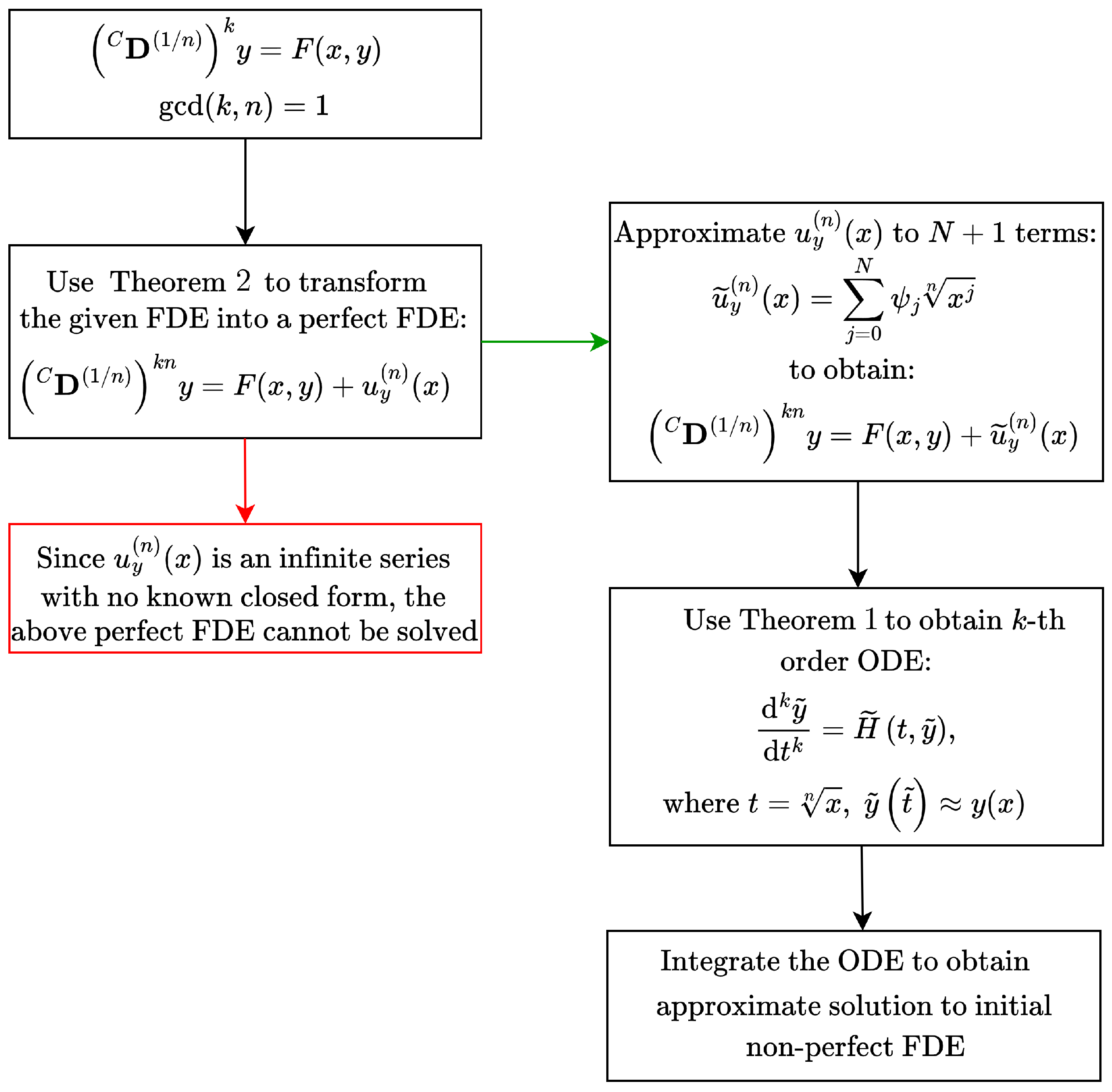
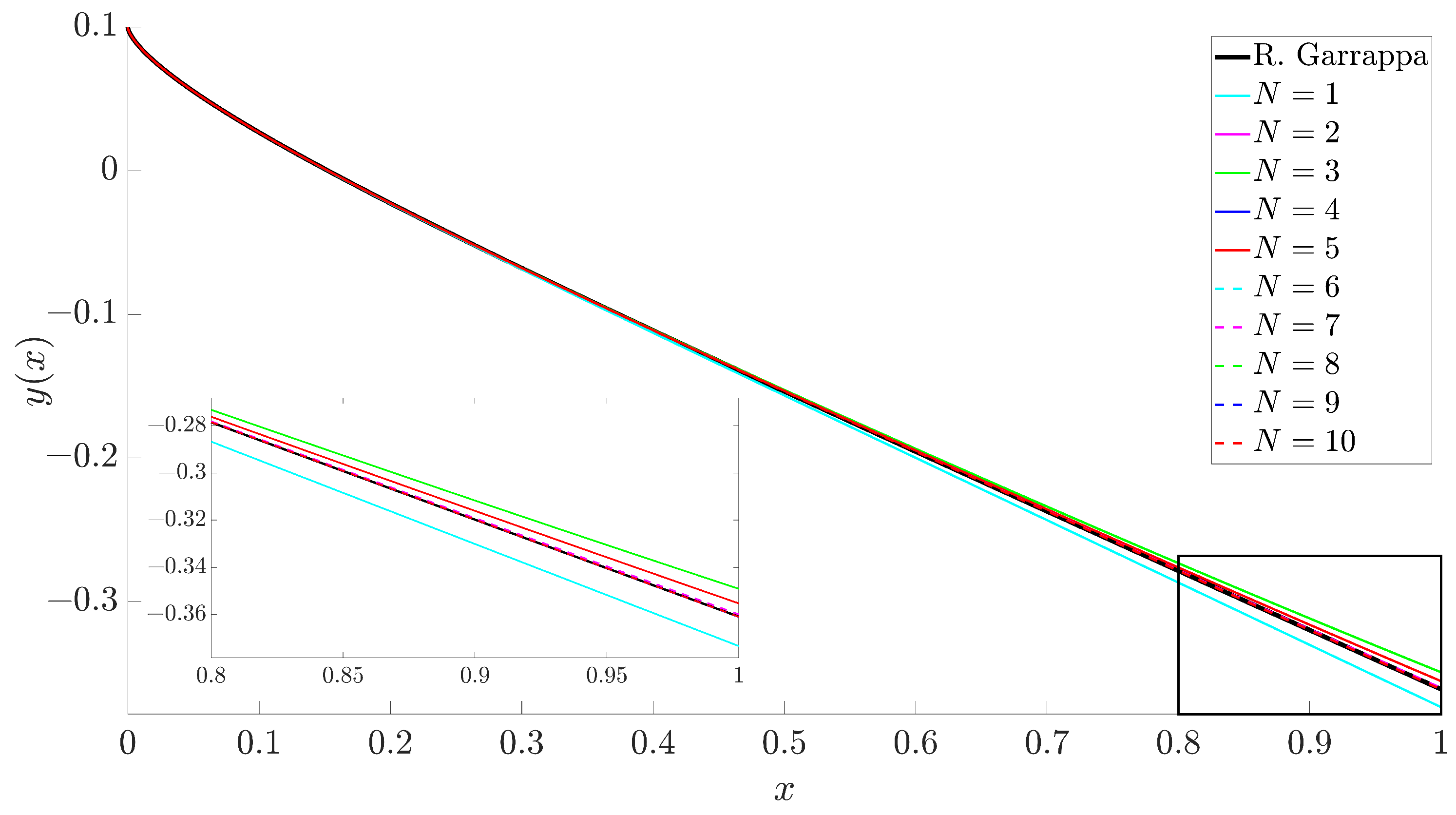
4. Numerical Application of the Proposed Approach

In this section, the feasibility of techniques presented in Section 3 is demonstrated by applying them to a specific Caputo FDE of the Riccati type. It is demonstrated that the approach agrees with well-known numerical methods.

Consider the following Riccati-type FDE:

$$\begin{array}{cc}\hfill & {\left({}^C\mathbf{D}^{(1/3)}\right)}^{2}y=-{\displaystyle \frac{1}{3}}+{\displaystyle \frac{1}{4}}{y}^2+{\displaystyle \frac{1}{2}}y,\hfill \\ \hfill & y\left(0\right)={\displaystyle \frac{1}{10}};{{}^C\mathbf{D}^{(1/3)}y|}_{x=0}=0.\hfill \end{array}$$

(68)

Using Theorem 2, the values of the parameters $d_k$ ($k=0,\dots ,4$) and $v_k$ ($k=0,\dots ,5$) can be computed as follows:

$$\begin{array}{cc}\hfill d_0& =2a_0^2{a}_2+a_0{a}_1^2+8a_0{a}_1{a}_2+4a_0{a}_2^2\hfill \\ \hfill & =2·{\left(-{\displaystyle \frac{1}{3}}\right)}^2·{\displaystyle \frac{1}{4}}+\left(-{\displaystyle \frac{1}{3}}\right)·{\left({\displaystyle \frac{1}{2}}\right)}^2+8·\left(-{\displaystyle \frac{1}{3}}\right)·{\displaystyle \frac{1}{2}}·{\displaystyle \frac{1}{4}}-4·{\displaystyle \frac{1}{3}}·{\left({\displaystyle \frac{1}{4}}\right)}^2=-{\displaystyle \frac{4}{9}};\hfill \\ \hfill d_1& =8a_0{a}_1{a}_2+16a_0{a}_2^2+a_1^3+8a_1^2{a}_2+4a_1{a}_2^2\hfill \\ \hfill & =8·\left(-{\displaystyle \frac{1}{3}}\right)·{\displaystyle \frac{1}{2}}·{\displaystyle \frac{1}{4}}+16·\left(-{\displaystyle \frac{1}{3}}\right)·{\left({\displaystyle \frac{1}{4}}\right)}^2+{\left({\displaystyle \frac{1}{2}}\right)}^3+8·{\left({\displaystyle \frac{1}{2}}\right)}^2·{\displaystyle \frac{1}{4}}\hfill \\ \hfill & +4·{\displaystyle \frac{1}{2}}·{\left({\displaystyle \frac{1}{4}}\right)}^2={\displaystyle \frac{1}{12}};\hfill \\ \hfill d_2& =8a_0{a}_2^2+7a_1^2{a}_2+24a_1{a}_2^2+4a_2^3\hfill \\ \hfill & =8·\left(-{\displaystyle \frac{1}{3}}\right)·{\left({\displaystyle \frac{1}{4}}\right)}^2+7·{\left({\displaystyle \frac{1}{2}}\right)}^2·{\displaystyle \frac{1}{4}}+24·{\displaystyle \frac{1}{2}}·{\left({\displaystyle \frac{1}{4}}\right)}^2+4·{\left({\displaystyle \frac{1}{4}}\right)}^3={\displaystyle \frac{13}{12}};\hfill \\ \hfill d_3& =12a_1{a}_2^2+16a_2^3=12·{\displaystyle \frac{1}{2}}·{\left({\displaystyle \frac{1}{4}}\right)}^2+16·{\left({\displaystyle \frac{1}{4}}\right)}^3={\displaystyle \frac{5}{8}};\hfill \\ \hfill d_4& =6a_2^3=6·{\left({\displaystyle \frac{1}{4}}\right)}^3={\displaystyle \frac{3}{32}};\hfill \\ \hfill v_0& ={\gamma }_0={\displaystyle \frac{1}{10}};\hfill \\ \hfill v_1& ={\gamma }_1=0;\hfill \\ \hfill v_2& =a_0+a_1{v}_0+a_2{v}_0^2={\displaystyle \frac{-337}{1200}};\hfill \\ \hfill v_3& =a_1{v}_1+a_2\left(\sum _{s=0}^1\left({\displaystyle \genfrac{}{}{0pt}{}{\frac{1}{3}}{\frac{s}{3}}}\right)v_s{v}_{1-s}\right)=0;\hfill \\ \hfill v_4& =a_1{v}_2+a_2\left(\sum _{s=0}^2\left({\displaystyle \genfrac{}{}{0pt}{}{\frac{2}{3}}{\frac{s}{3}}}\right)v_s{v}_{2-s}\right)={\displaystyle \frac{-3707}{\mathrm{24,000}}};\hfill \\ \hfill v_5& =a_1{v}_3+a_2\left(\sum _{s=0}^3\left({\displaystyle \genfrac{}{}{0pt}{}{\frac{3}{3}}{\frac{s}{3}}}\right)v_s{v}_{3-s}\right)=0.\hfill \end{array}$$

(69)

Therefore, (68) can be transformed into the following perfect Cauchy problem:

$$\begin{array}{cc}\hfill & {\left({}^C\mathbf{D}^{(1/3)}\right)}^{6}y=-{\displaystyle \frac{4}{9}}+{\displaystyle \frac{1}{12}}y+{\displaystyle \frac{13}{12}}{y}^2+{\displaystyle \frac{5}{8}}{y}^3+{\displaystyle \frac{3}{32}}{y}^4+u_y^{\left(3\right)}\left(x\right),\hfill \\ \hfill & y\left(0\right)={\displaystyle \frac{1}{10}};{{}^C\mathbf{D}^{(1/3)}y|}_{x=0}=0,{{\left({}^C\mathbf{D}^{(1/3)}\right)}^{2}y|}_{x=0}=-{\displaystyle \frac{337}{1200}},\hfill \\ \hfill & {{\left({}^C\mathbf{D}^{(1/3)}\right)}^{3}y|}_{x=0}=0,{{\left({}^C\mathbf{D}^{(1/3)}\right)}^{4}y|}_{x=0}=-{\displaystyle \frac{3707}{\mathrm{24,000}}},{{\left({}^C\mathbf{D}^{(1/3)}\right)}^{5}y|}_{x=0}=0.\hfill \end{array}$$

(70)

where the coefficients of the function $u_y^{\left(3\right)}\left(x\right)={\sum }_{j=0}^{+\infty }{\kappa }_j{w}_j^{\left(3\right)}$ are obtained using relations (57)–(59).

Using Theorem 1, (70) can be converted into the following second-order ODE:

$$\begin{array}{c}t{\displaystyle \frac{{\mathrm{d}}^2\widehat{y}}{\mathrm{d}{t}^2}}-2\frac{\mathrm{d}\widehat{y}}{\mathrm{d}t}-{\displaystyle \frac{337}{600\Gamma (5/3)}}t+{\displaystyle \frac{3707}{6000\Gamma (7/3)}}{t}^3\hfill \\ =9t^5\left(-{\displaystyle \frac{4}{9}}+{\displaystyle \frac{1}{12}}\widehat{y}+{\displaystyle \frac{13}{12}}{\widehat{y}}^2+{\displaystyle \frac{5}{8}}{\widehat{y}}^3+{\displaystyle \frac{3}{32}}{\widehat{y}}^4+u_y^{\left(3\right)}\left(t^3\right)\right);\hfill \\ \widehat{y}\left(0\right)={\displaystyle \frac{1}{10}};{\widehat{y}}^{\prime }\left(0\right)=0,\hfill \end{array}$$

(71)

where $t=\sqrt[3]{x}$ and $\widehat{y}=\widehat{y}\left(t\right)=y\left(x\right)$. Note that the function $u_y^{\left(3\right)}\left(t^3\right)$ can only be represented by an infinite power series. Therefore, in order to solve the above ODE, $u_y^{\left(3\right)}\left(t^3\right)$ is approximated by taking the first $N+1$ terms:

$$\begin{array}{cc}\hfill & t{\displaystyle \frac{{\mathrm{d}}^2\tilde{y}}{\mathrm{d}{t}^2}}-2\frac{\mathrm{d}\tilde{y}}{\mathrm{d}t}-{\displaystyle \frac{337}{600\Gamma (5/3)}}t+{\displaystyle \frac{3707}{6000\Gamma (7/3)}}{t}^3\hfill \\ \hfill & =9t^5\left(-{\displaystyle \frac{4}{9}}+{\displaystyle \frac{1}{12}}\tilde{y}+{\displaystyle \frac{13}{12}}{\tilde{y}}^2+{\displaystyle \frac{5}{8}}{\tilde{y}}^3+{\displaystyle \frac{3}{32}}{\tilde{y}}^4+\sum _{j=0}^N{\kappa }_j{\displaystyle \frac{t^j}{\Gamma \left(1+\frac{j}{3}\right)}}\right);\hfill \\ \hfill & \tilde{y}\left(0\right)={\displaystyle \frac{1}{10}};{\tilde{y}}^{\prime }\left(0\right)=0,\hfill \end{array}$$

(72)

where $\tilde{y}\to \widehat{y}$ as $N\to \infty$.

The solution to (68) is obtained via constructing a numerical solution to (72) and applying the transformation $x=t^3$ to obtain the approximate FDE solution. Solutions for various selections of the order N up to which $u_y^{\left(3\right)}$ is evaluated are depicted in Figure 2. It can be observed that the solutions constructed via the presented method agree with the well-known R. Garrappa’s FDE integration algorithm [34].

It should be noted that the numerical efficiency and complexity of the presented technique is intrinsically tied to the integrator that is used to obtain a numerical solution to (72). This is due to the fact that once a solution to ODE (72) is obtained, the solution to FDE (68) is approximated using the nonlinear time transformation $x=t^n$.

Another factor in efficiency is the number of terms used to approximate $u_y^{\left(3\right)}\left(x\right)$ in (70). Naturally, adding an extra term results in a penalty with respect to computation; however, accuracy is also increased as shown in Figure 2.

While the presented technique has many advantages, such as the ability to select any desired ODE solver (numerical or otherwise), there are some limitations. Firstly, only equations of Caputo differentiation order ${\displaystyle \frac{k}{n}}$ can be considered, so any irrational fractional differentiation order cannot be used unless approximated via a simple fraction. Moreover, a selection of non-analytical function $Q\left(y\right)$ in the FDE would also require an altered approach not covered in this paper.

5. Concluding Remarks

A novel approach for solving ${\left({}^C\mathbf{D}^{(1/n)}\right)}^k$-type fractional differential equations (FDEs) has been presented. The main contribution of this work is the extension of fractional power series techniques beyond the previously studied ${}^C\mathbf{D}^{(1/n)}$-type FDEs [30] to encompass ${\left({}^C\mathbf{D}^{(1/n)}\right)}^k$-type equations.

The concept of perfect FDEs is extended to equations of the form

$${\left({}^C\mathbf{D}^{(1/n)}\right)}^{kn}y=Q\left(y\right),$$

(73)

which, as demonstrated, can be transformed into k-th order ODEs.

The proposed methodology enables the transformation of ${\left({}^C\mathbf{D}^{(1/n)}\right)}^k$-type FDEs into ${\left({}^C\mathbf{D}^{(1/n)}\right)}^{kn}$-type equations, which can then be further reduced to k-th order ordinary differential equations (ODEs). Consequently, the framework broadens the class of FDEs that can be treated semi-analytically, providing new avenues for obtaining semi-analytical solutions in cases where only numerical approximations were previously available. The effectiveness of the proposed framework is demonstrated through its application to a fractional Riccati-type differential equation.

Furthermore, the presented approach can also be used numerically, as demonstrated in Section 4. Due to this, the techniques developed in this paper are widely applicable and can be used in any research field that uses Caputo FDEs with a rational differentiation order ${\displaystyle \frac{k}{n}}<1$ to model real-world processes. Moreover, since the FDE solution is approximated by an ODE solution, any of the myriad numerical integration methods can be applied in conjunction with the presented approach.

Compared to prior work, including direct numerical schemes for FDEs (such as finite difference or predictor–corrector methods) and the authors’ previous work limited to ${}^C\mathbf{D}^{(1/n)}$-type equations [29,30], the distinct aspect of the current methodology lies in its ability to handle the more general ${\left({}^C\mathbf{D}^{(1/n)}\right)}^k$ operator structure. The key contribution is the systematic transformation of this broader class of FDEs into equivalent, albeit potentially complex, k-th order ODEs. This transformation is significant because it recasts the fractional problem into the domain of ordinary differential equations, potentially simplifying the analysis and solution process. Unlike purely numerical FDE solvers which provide discrete approximations, this operator-based approach, through the intermediary ODE, can offer semi-analytical insights and leverages the extensive toolkit available for solving ODEs, both analytically (in specific cases) and numerically, offering flexibility in implementation. This contrasts with methods that directly use the fractional operator, which often require specialized numerical techniques and may obscure underlying structural similarities to integer-order systems.

References

1. Li, X.P.; Alrihieli, H.F.; Algehyne, E.A.; Khan, M.A.; Alshahrani, M.Y.; Alraey, Y.; Riaz, M.B. Application of piecewise fractional differential equation to COVID-19 infection dynamics. Results Phys. 2022, 39, 105685. [Google Scholar] [CrossRef]
2. Farman, M.; Xu, C.; Shehzad, A.; Akgul, A. Modeling and dynamics of measles via fractional differential operator of singular and non-singular kernels. Math. Comput. Simul. 2024, 221, 461–488. [Google Scholar]
3. Edward, S. A fractional order model for the transmission dynamics of shigellosis. Heliyon 2024, 10, e31242. [Google Scholar] [CrossRef] [PubMed]
4. Mahdy, A.M.; Almalki, N.; Higazy, M. A general fractional breast cancer model: Model graph energy, Caputo-Fabrizio derivative existence and uniqueness plus numerical simulation. Partial Differ. Eq. Appl. Math. 2024, 10, 100723. [Google Scholar] [CrossRef]
5. Agarwal, R.; Airan, P.; Agarwal, R.P. Exploring the Landscape of Fractional-Order Models in Epidemiology: A Comparative Simulation Study. Axioms 2024, 13, 545. [Google Scholar] [CrossRef]
6. Chauhan, R.; Singh, R.; Kumar, A.; Thakur, N.K. Role of prey refuge and fear level in fractional prey–predator model with anti-predator. J. Comput. Sci. 2024, 81, 102385. [Google Scholar] [CrossRef]
7. Singh, J.; Agrawal, R.; Baleanu, D. Dynamical analysis of fractional order biological population model with carrying capacity under Caputo-Katugampola memory. Alex. Eng. J. 2024, 91, 394–402. [Google Scholar] [CrossRef]
8. Matouk, A. Applications of the generalized gamma function to a fractional-order biological system. Heliyon 2023, 9, e18645. [Google Scholar] [CrossRef]
9. Seralan, V.; Vadivel, R.; Gunasekaran, N.; Radwan, T. Dynamics of Fractional-Order Three-Species Food Chain Model with Vigilance Effect. Fractal Fract. 2025, 9, 45. [Google Scholar] [CrossRef]
10. Li, H.; ur Rahman, G.; Naz, H.; Gómez-Aguilar, J. Modeling of implicit multi term fractional delay differential equation: Application in pollutant dispersion problem. Alex. Eng. J. 2024, 94, 1–22. [Google Scholar] [CrossRef]
11. Zhang, X.; Gao, X.; Duan, L.; Gong, Q.; Wang, Y.; Ao, X. A novel method for state of health estimation of lithium-ion batteries based on fractional-order differential voltage-capacity curve. Appl. Energy 2025, 377, 124404. [Google Scholar]
12. Jornet, M.; Nieto, J.J. On a nonlinear stochastic fractional differential equation of fluid dynamics. Phys. D Nonlinear Phenom. 2024, 470, 134400. [Google Scholar]
13. Huseynov, I.T.; Mahmudov, N.I. A class of Langevin time-delay differential equations with general fractional orders and their applications to vibration theory. J. King Saud Univ.-Sci. 2021, 33, 101596. [Google Scholar] [CrossRef]
14. Abdou, M.A. An analytical method for space–time fractional nonlinear differential equations arising in plasma physics. J. Ocean Eng. Sci. 2017, 2, 288–292. [Google Scholar]
15. Srivastava, H.M.; Adel, W.; Izadi, M.; El-Sayed, A.A. Solving some physics problems involving fractional-order differential equations with the Morgan-Voyce polynomials. Fractal Fract. 2023, 7, 301. [Google Scholar] [CrossRef]
16. Hilfer, R. Applications of Fractional Calculus in Physics; World Scientific: Singapore; River Edge, NJ, USA, 2000. [Google Scholar]
17. Graef, J.R.; Kong, L.; Ledoan, A.; Wang, M. Stability analysis of a fractional online social network model. Math. Comput. Simul. 2020, 178, 625–645. [Google Scholar]
18. Jin, T.; Yang, X. Monotonicity theorem for the uncertain fractional differential equation and application to uncertain financial market. Math. Comput. Simul. 2021, 190, 203–221. [Google Scholar]
19. Kumar, Y.; Singh, V.K. Computational approach based on wavelets for financial mathematical model governed by distributed order fractional differential equation. Math. Comput. Simul. 2021, 190, 531–569. [Google Scholar]
20. Sene, N. Analytical investigations of the fractional free convection flow of Brinkman type fluid described by the Caputo fractional derivative. Results Phys. 2022, 37, 105555. [Google Scholar]
21. Sawangtong, W.; Sawangtong, P. An analytical solution for the Caputo type generalized fractional evolution equation. Alex. Eng. J. 2022, 61, 5475–5483. [Google Scholar]
22. Hassan, A.; Arafa, A.; Rida, S.; Dagher, M.; El Sherbiny, H. Adapting semi-analytical treatments to the time-fractional derivative Gardner and Cahn-Hilliard equations. Alex. Eng. J. 2024, 87, 389–397. [Google Scholar]
23. Fan, Z.Y.; Ali, K.K.; Maneea, M.; Inc, M.; Yao, S.W. Solution of time fractional Fitzhugh–Nagumo equation using semi analytical techniques. Results Phys. 2023, 51, 106679. [Google Scholar]
24. Kheybari, S.; Darvishi, M.T.; Hashemi, M.S. A semi-analytical approach to Caputo type time-fractional modified anomalous sub-diffusion equations. Appl. Numer. Math. 2020, 158, 103–122. [Google Scholar]
25. Li, C.; N’Gbo, N.; Su, F. Finite difference methods for nonlinear fractional differential equation with ψ-Caputo derivative. Phys. D Nonlinear Phenom. 2024, 460, 134103. [Google Scholar]
26. Sivalingam, S.; Kumar, P.; Trinh, H.; Govindaraj, V. A novel L1-Predictor-Corrector method for the numerical solution of the generalized-Caputo type fractional differential equations. Math. Comput. Simul. 2024, 220, 462–480. [Google Scholar]
27. Saeed, U.; ur Rehman, M. A new scheme for the solution of the nonlinear Caputo–Hadamard fractional differential equations. Alex. Eng. J. 2024, 105, 56–69. [Google Scholar]
28. Raghavendran, P.; Gunasekar, T.; Gochhait, S. Application of artificial neural networks for existence and controllability in impulsive fractional Volterra-Fredholm integro-differential equations. Appl. Math. Sci. Eng. 2024, 32, 2436440. [Google Scholar]
29. Navickas, Z.; Telksnys, T.; Marcinkevicius, R.; Ragulskis, M. Operator-based approach for the construction of analytical soliton solutions to nonlinear fractional-order differential equations. Chaos Solitons Fractals 2017, 104, 625–634. [Google Scholar]
30. Marcinkevicius, R.; Telksniene, I.; Telksnys, T.; Navickas, Z.; Ragulskis, M. The construction of solutions to CD(1/n) type FDEs via reduction to (CD(1/n))n type FDEs. AIMS Math. 2022, 7, 16536–16554. [Google Scholar] [CrossRef]
31. Timofejeva, I.; Navickas, Z.; Telksnys, T.; Marcinkevicius, R.; Ragulskis, M. An Operator-Based Scheme for the Numerical Integration of FDEs. Mathematics 2021, 9, 1372. [Google Scholar] [CrossRef]
32. Navickas, Z.; Telksnys, T.; Timofejeva, I.; Marcinkevicius, R.; Ragulskis, M. The Fractal Structure of Analytical Solutions to Fractional Riccati Equation. Fractals 2023, 32, 2340130. [Google Scholar] [CrossRef]
33. Formichella, S.; Straub, A. Gaussian binomial coefficients with negative arguments. Ann. Comb. 2019, 23, 725–748. [Google Scholar]
34. Garrappa, R. Numerical solution of fractional differential equations: A survey and a software tutorial. Mathematics 2018, 6, 16. [Google Scholar] [CrossRef]
Figure 1. Schematic diagram of construction of solutions to FDEs of type D ( 1 / n ) C k y = F ( x , y ) .
Mathematics 13 01169 g001
Figure 2. Convergence study for the numerical solution of (68). The reference solution, obtained via Garrappa’s FDE algorithm [34], is shown by the solid black line. The remaining lines illustrate approximate solutions generated by the presented method for varying approximation orders, N = 1 , 2 , , 10 . A zoomed view of the final segment is provided on the bottom-left inset for enhanced detail.
Mathematics 13 01169 g002
Disclaimer/Publisher’s Note: The statements, opinions and data contained in all publications are solely those of the individual author(s) and contributor(s) and not of MDPI and/or the editor(s). MDPI and/or the editor(s) disclaim responsibility for any injury to people or property resulting from any ideas, methods, instructions or products referred to in the content.