Pontryagin’s Principle-Based Algorithms for Optimal Control Problems of Parabolic Equations

Abstract

This paper applies the Method of Successive Approximations (MSA) based on Pontryagin’s principle to solve optimal control problems with state constraints for semilinear parabolic equations. Error estimates for the first and second derivatives of the function are derived under $L^{\infty }$-bounded conditions. An augmented MSA is developed using the augmented Lagrangian method, and its convergence is proven. The effectiveness of the proposed method is demonstrated through numerical experiments.

1. Introduction

In this paper, we investigate the optimal control problem for parabolic equations with state constraints and Neumann boundary conditions, formulated as follows:

$$\begin{array}{cc}\hfill \underset{u,v}{min}J(y,u,v):=& {\int }_{{\Omega }_T}F(x,t,y,u)dxdt+{\int }_{{\Sigma }_T}G(s,t,y,v)dsdt\hfill \\ \hfill & +{\int }_{\Omega }L(x,y(x,T))dx,\hfill \end{array}$$

(1)

subject to the dynamics

$$\begin{array}{cc}\hfill {\displaystyle \frac{\partial y}{\partial t}}+Ay+f(x,t,y,u)& =0,\mathrm{in}{\Omega }_T,\hfill \\ \hfill {\displaystyle \frac{\partial y}{\partial n_A}}+v& =0,\mathrm{on}{\Sigma }_T,\hfill \\ \hfill y(·,0)& =y_0,\mathrm{in}\overline{\Omega },\hfill \end{array}$$

where A is a second-order elliptic operator. The specific problem setup is described in Section 2.1.

The solution methods most commonly employed to address such problems include solving the Hamilton–Jacobi–Bellman (HJB) equation [1,2] and utilizing the Pontryagin maximum principle [3,4]. Although both approaches have been extensively studied, analytical solutions are generally unavailable for most practical cases, leading to the development of various numerical methods.

Current numerical techniques for solving the HJB equation include semi-Lagrangian schemes [2], sparse grid approaches [5], tensor-calculus-based methods [6], and successive Galerkin approximations [7,8,9,10]. Notably, policy iteration and Howard’s algorithm [11,12,13] are discrete implementations of the continuous Galerkin method. In the numerical solution of Pontryagin’s optimality principle, approaches such as the two-point boundary value problem method [14,15], collocation methods combined with nonlinear programming techniques [16,17,18,19], and the Method of Successive Approximations (MSA) [20] are often applied.

MSA plays a crucial role in the numerical resolution of both types of problems, as it is an iterative procedure based on alternating propagation and optimization steps. In [21], MSA is employed to solve optimal control problems governed by ordinary differential equations, with an extended version derived via the augmented Lagrangian method [22]. Additionally, in [23], a modified version of MSA for stochastic control problems is proposed, and convergence of the algorithm is established. In this paper, we provide an error estimate for MSA applied to optimal control problems of parabolic equations under specific conditions (see Lemma 3) and propose the corresponding augmented MSA.

The structure of this paper is as follows: In Section 2, we present preliminary results related to the original problem (1) and the corresponding Pontryagin maximum principle. In Section 3, we apply the Method of Successive Approximations (MSA) and its improved variant to solve the problem. Specifically, in Section 3.1, we introduce the basic MSA based on the Pontryagin principle; in Section 3.2, we state certain assumptions under which we derive the error estimate for the basic MSA; in Section 3.3, we introduce the augmented Pontryagin principle and the augmented MSA based on it; and in Section 3.4, we prove the convergence of the augmented MSA. Finally, in Section 4, we demonstrate the effectiveness of the augmented MSA through numerical experiments.

Notation Throughout this paper, ${(·,·)}_{\Omega }$ denotes the inner product in $L^2(\Omega )$, and ${(·,·)}_{\Gamma }$ denotes the inner product in $L^2(\Gamma )$. The constant C appearing in the text may represent different values and will be adjusted as necessary.

2. Preliminary Results

2.1. Problem Setting

Let $\Omega \subset {\mathbb{R}}^N$ be an open, bounded subset of ${\mathbb{R}}^N$ with a $C^{2,\beta }$-boundary, where $N\in \{2,3\}$. That is, the boundary $\partial \Omega$ is a $(N-1)$-dimensional manifold of class $C^{2,\beta }$, and $\Omega$ lies locally on one side of its boundary. A function is said to be of class $C^{2,\beta }$ if it is of class $C^2$ and its second-order partial derivatives are Hölder continuous with exponent $\beta$. For a fixed time interval $T>0$, we define the space–time domain ${\Omega }_T:=\Omega \times (0,T)$ and its lateral boundary ${\Sigma }_T:=\partial \Omega \times (0,T)$.

The function space $\mathcal{Y}$ is given by

$$\mathcal{Y}:=\mathcal{W}(0,T;L^2(\Omega ),H^1(\Omega ))\cap C\left({\overline{\Omega }}_T\right),$$

where $\mathcal{W}(0,T;L^2(\Omega ),H^1(\Omega ))$ denotes the Hilbert space of functions y such that $y\in L^2(0,T;H^1(\Omega ))$ and $y_t\in L^2(0,T;H^{-1}(\Omega ))$. The associated norm is defined by

$${\parallel y\parallel }_{\mathcal{W}(0,T;L^2(\Omega ),H^1(\Omega ))}:=\sqrt{{\parallel y\parallel }_{L^2(0,T;H^1(\Omega ))}^2+{\parallel y_t\parallel }_{L^2(0,T;H^{-1}(\Omega ))}^2}.$$

The control spaces are defined as $\mathcal{U}:=L^r\left({\Omega }_T\right)$ and $\mathcal{V}:=L^q\left({\Sigma }_T\right)$, where the exponents $r>{\displaystyle \frac{N}{2}}+1$ and $q>N+1$ ensure the required regularity and integrability conditions.

Consider the second-order differential operator A given by

$$Ay(x,t)=-\sum _{i,j=1}^N{\partial }_{x_j}\left(a_{ij}\left(x\right){\partial }_{x_i}y(x,t)\right),$$

where the coefficients $a_{ij}\left(x\right)\in L^{\infty }(\Omega )$ satisfy $a_{ij}\left(x\right)=a_{ji}\left(x\right)$ for all $i,j$. The operator A is assumed to be uniformly elliptic, meaning there exists a constant $K>0$ such that

$$\sum _{i,j=1}^N{a}_{ij}\left(x\right){\xi }_i{\xi }_j\ge K{\parallel \xi \parallel }^2\mathrm{for}\mathrm{almost}\mathrm{every}x\in \Omega \mathrm{and}\mathrm{all}\xi \in {\mathbb{R}}^N.$$

The goal is to minimize the cost functional

$$\begin{array}{cc}\hfill J(y,u,v):=& {\int }_{{\Omega }_T}F(x,t,y,u)dxdt+{\int }_{{\Sigma }_T}G(s,t,y,v)dsdt\hfill \\ \hfill & +{\int }_{\Omega }L(x,y(x,T))dx,\hfill \end{array}$$

(2)

subject to the parabolic system

$$\begin{array}{cc}\hfill {\displaystyle \frac{\partial y}{\partial t}}+Ay+f(x,t,y,u)& =0,\mathrm{in}{\Omega }_T,\hfill \\ \hfill {\displaystyle \frac{\partial y}{\partial n_A}}+v& =0,\mathrm{on}{\Sigma }_T,\hfill \\ \hfill y(·,0)& =y_0,\mathrm{in}\overline{\Omega },\hfill \end{array}$$

(3)

where the conormal derivative is given by

$${\displaystyle \frac{\partial y}{\partial n_A}}(x,t)=\sum _{i,j=1}^N{a}_{ij}\left(x\right){\partial }_{x_i}y(x,t){\nu }_j\left(x\right),$$

and $\nu =({\nu }_1, \dots , {\nu }_N)$ denotes the unit outward normal vector to $\Gamma$.

The following assumption applies throughout this paper, and the functions f, F, G, and L are assumed to satisfy the conditions below.

Assumption 1. 

Let $M_1(·,·)\in L^r\left({\Omega }_T\right)$, $M_2(·)\in L^1(\Omega )$, $M_3>0$, $M_4(·,·)\in L^1\left({\Omega }_T\right)$, $M_5(·,·)\in L^1\left({\Sigma }_T\right)$, $M_6(·,·)\in L^q\left({\Sigma }_T\right)$, and $\eta \left(\right|·\left|\right)$ be a nondecreasing function mapping ${\mathbb{R}}^{+}$ to ${\mathbb{R}}^{+}$. Furthermore, let $m_1>0$ and $C_0>0$. The following conditions hold:

1. 

The function $f(x,t,y,u)$:

- For every $(y,u)\in {\mathbb{R}}^2$, $f(·,·,y,u)$ is measurable on ${\Omega }_T$.

- For almost every $(x,t)\in {\Omega }_T$, $f(x,t,·,·)$ is continuous on $\mathbb{R}\times \mathbb{R}$.

- For almost every $(x,t)\in {\Omega }_T$ and every $u\in \mathbb{R}$, $f(x,t,·,u)$ is of class $C^2$ on $\mathbb{R}$.

- For almost every $(x,t)\in {\Omega }_T$,

$$\left|f(x,t,0,u)\right|\le M_1(x,t)+m_1\left|u\right|,$$

$$C_0\le f_y^{\prime }(x,t,y,u)\le (M_1(x,t)+m_1\left|u\right|\left)\eta \right(\left|y\right|).$$

2. 

The function $L(x,y)$:

- For every $y\in \mathbb{R}$, $L(·,y)$ is measurable on Ω.

- For almost every $x\in \Omega$, $L(x,·)$ is continuous on $\mathbb{R}$ and is of class $C^2$ on $\mathbb{R}$.

- For almost every $x\in \Omega$,

$$\left|L(x,0)\right|\le M_2\left(x\right),|L_y^{\prime }(x,y)|\le M_3\eta \left(\right|y\left|\right),$$

$$|L_y^{\prime }(x,y)-L_y^{\prime }(x,z)|\le M_3\eta \left(\right|y\left|\right)\eta \left(\right|z\left|\right).$$

3. 

The function $F(x,t,y,u)$:

- For every $(y,u)\in {\mathbb{R}}^2$, $F(·,·,y,u)$ is measurable on ${\Omega }_T$.

- For almost every $(x,t)\in {\Omega }_T$, $F(x,t,·,·)$ is continuous on $\mathbb{R}\times \mathbb{R}$.

- For almost every $(x,t)\in {\Omega }_T$ and every $u\in \mathbb{R}$, $F(x,t,·,u)$ is of class $C^2$ on $\mathbb{R}$.

- For almost every $(x,t)\in {\Omega }_T$,

$$\left|F(x,t,0,u)\right|\le M_4(x,t)+m_1{\left|u\right|}^r,|F_y^{\prime }(x,t,y,u)|\le (M_1(x,t)+m_1\left|u\right|\left)\eta \right(\left|y\right|).$$

4. 

The function $G(s,t,y,v)$:

- For every $(y,v)\in {\mathbb{R}}^2$, $G(·,·,y,v)$ is measurable on ${\Sigma }_T$.

- For almost every $(s,t)\in {\Sigma }_T$, $G(s,t,·,·)$ is continuous on $\mathbb{R}\times \mathbb{R}$.

- For almost every $(s,t)\in {\Sigma }_T$ and every $v\in \mathbb{R}$, $G(s,t,·,v)$ is of class $C^2$ on $\mathbb{R}$.

- For almost every $(s,t)\in {\Sigma }_T$,

$$\left|G(s,t,0,v)\right|\le M_5(s,t)+m_1{\left|v\right|}^q,|G_y^{\prime }(s,t,y,v)|\le (M_6(s,t)+m_1\left|v\right|\left)\eta \right(\left|y\right|).$$

2.2. Pontryagin’s Principle

In this section, we will introduce the first-order necessity condition for (1), which is Pontryagin’s principle. The complete proof process of Pontryagin’s principle of the control problem governed by the semilinear parabolic equation involved in this paper is given in [4].

First, we define the Hamiltonian function expression of (1), including the distribution Hamiltonian function and the boundary Hamiltonian function, and the expression is as follows:

$$H_{{\Omega }_T}(x,t,y,u,p):=F(x,t,y,u)-pf(x,t,y,u),$$

for every $(x,t,y,u,p)\in \Omega \times (0,T)\times R\times R\times R,$

$$H_{{\Sigma }_T}(x,t,y,v,p):=G(s,t,y,v)-pv,$$

for every $(s,t,y,v,p)\in \Sigma \times (0,T)\times R\times R\times R$.

Theorem 1. 

Let $(\overline{y},\overline{u},\overline{v})$ be the solution of $\left(P\right)$. Then there exists a unique adjoint state $\overline{p}\in \mathcal{W}(0,T;L^2(\Omega ),H^1(\Omega ))\cap C\left({\Omega }_T\right)$, satisfying the following equation:

$$\begin{array}{ccc}\hfill -{\displaystyle \frac{\partial p}{\partial t}}+Ap+f_y^{\prime }(x,t,\overline{y},\overline{u})p& =F_y^{\prime }(x,t,\overline{y},\overline{u}),\hfill & \hfill \mathrm{in}{\Omega }_T,\\ \hfill {\displaystyle \frac{\partial p}{\partial n_A}}& =G_y^{\prime }(s,t,\overline{y},\overline{v}),\hfill & \hfill \mathrm{on}{\Sigma }_T,\\ \hfill p(·,T)& =L_y^{\prime }(x,y(·,T)),\hfill & \hfill \mathrm{in}\Omega .\end{array}$$

(4)

such that

$$\begin{array}{cc}\hfill & H_{{\Omega }_T}(x,t,\overline{y},\overline{u},\overline{p})=\underset{u\in \mathcal{U}}{min}{H}_{{\Omega }_T}(x,t,\overline{y},u,\overline{p}),\hfill \\ \hfill & \mathrm{for}\mathrm{a}.\mathrm{e}.(x,t)\in {\Omega }_T,\hfill \\ \hfill & H_{{\Sigma }_T}(s,t,\overline{y},\overline{v},\overline{p})=\underset{v\in \mathcal{V}}{min}{H}_{{\Sigma }_T}(s,t,\overline{y},v,\overline{p}),\hfill \\ \hfill & \mathrm{for}\mathrm{a}.\mathrm{e}.(s,t)\in {\Sigma }_T.\hfill \end{array}$$

Proof. 

See Theorem 2.1 of [4].    □

3. Method of Successive Approximations

In this section, we propose a numerical algorithm to solve Problem (1) based on the maximum principle. The algorithm’s error analysis and convergence properties will be examined in the framework of continuous time and space. To achieve this, we employ the Method of Successive Approximations (MSA), initially introduced by Chernousko and Lyubushin in [20]. Below, we present the fundamental formulation of the method.

3.1. Basic MSA

The basic MSA alternates between solving the state equation and the adjoint equation, followed by an optimization step to update the control variables. In this approach, the state equation captures the system’s dynamics, while the adjoint equation provides gradient information essential for optimizing the Hamiltonian. At each iteration, the control variables are updated by minimizing the Hamiltonian over the admissible control sets. This iterative process is repeated until a predefined termination criterion is met, ensuring convergence under suitable conditions. The detailed steps of the algorithm are presented in Algorithm 1 below.

Algorithm 1: Basic MSA

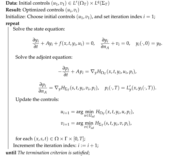    The convergence of the basic MSA has been established for a limited class of linear quadratic regulators [24]. However, it is well documented that the method often diverges in more general settings, particularly when unfavorable initial controls are chosen [20,24]. This divergence underscores the need to understand the instability of the algorithm, specifically the relationship between the maximization step in Algorithm 1 and the underlying optimization problem (1). To address this issue, our goal is to modify the basic MSA to ensure robust convergence, even under less favorable conditions.

3.2. Error Estimate

In this section, we establish the relationship between the control index J and the minimization of the Hamiltonian through a lemma. Prior to this, we introduce the necessary assumptions.

Assumption 2. 

For every $y\in \mathcal{Y}$, $u\in \mathcal{U}$, and $v\in \mathcal{V}$, the first-order and second-order derivatives of f, L, F, and G satisfy the following:

$$\Vert f_y^{\prime }{(·,·,y,u)\Vert }_{L^{\infty }\left({\Omega }_T\right)}\le C_1,{\Vert f_{yy}^{\prime \prime }(·,·,y,u)\Vert }_{L^{\infty }\left({\Omega }_T\right)}\le C_2,$$

$$\Vert F_y^{\prime }{(·,·,y,u)\Vert }_{L^{\infty }\left({\Omega }_T\right)}\le C_3,{\Vert F_{yy}^{\prime \prime }(·,·,y,u)\Vert }_{L^{\infty }\left({\Omega }_T\right)}\le C_4,$$

$$\Vert L_y^{\prime }{(·,y)\Vert }_{L^{\infty }(\Omega )}\le C_5,{\Vert L_{yy}^{\prime \prime }(·,y)\Vert }_{L^{\infty }(\Omega )}\le C_6,$$

$$\Vert G_y^{\prime }{(·,·,y,v)\Vert }_{L^{\infty }\left({\Sigma }_T\right)}\le C_7,{\Vert G_{yy}^{\prime \prime }(·,·,y,v)\Vert }_{L^{\infty }\left({\Omega }_T\right)}\le C_8,$$

where $C>0$ is a constant.

Before deriving the error estimate, we first establish upper bounds for $p^{\theta }$ and $\delta y$ under their respective norms. These bounds are obtained through the following two lemmas. Here, we denote $y^{\theta }:=y(u^{\theta },v^{\theta })$, $y^{\varphi }:=y(u^{\varphi },v^{\varphi })$, $\delta y:=y^{\varphi }-y^{\theta }$, and $p^{\theta }:=p(u^{\theta },v^{\theta },y^{\theta })$.

Lemma 1. 

Let Assumption 1 hold. Then, there exists a constant $C_9$ such that

$$\begin{array}{c}\hfill \Vert p^{\theta }{\Vert }_{L^{\infty }\left({\Omega }_T\right)}\le C_9.\end{array}$$

(5)

Proof. 

Refer to Proposition 4.1 of [4], along with the embedding $L^r\left({\Omega }_T\right)\hookrightarrow L^{\infty }\left({\Omega }_T\right)$ and $L^s\left({\Sigma }_T\right)\hookrightarrow L^{\infty }\left({\Sigma }_T\right)$, to obtain the result.    □

Lemma 2. 

Let Assumptions 1 and 2 be fulfilled. Then, there exist constants $C_{10}>0$ such that

$$\begin{array}{cc}\hfill & {\Vert \delta y\Vert }_{L^2\left({\Omega }_T\right)}^2+{\Vert \delta y\Vert }_{L^2\left({\Sigma }_T\right)}^2\le C_{10}({\Vert v^{\varphi }-v^{\theta }\Vert }_{L^2\left({\Sigma }_T\right)}^2\hfill \\ \hfill & +\Vert f(·,·,y^{\theta },u^{\varphi })-f(·,·,y^{\theta },u^{\theta }){\Vert }_{L^2\left({\Omega }_T\right)}^2).\hfill \end{array}$$

(6)

Proof. 

By multiplying both sides of the parabolic Equation (3) corresponding to $\delta y$ by $\delta y$ and integrating over $\Omega$, we obtain

$$\begin{array}{cc}\hfill & {({\displaystyle \frac{\partial \delta y}{\partial t}},\delta y)}_{\Omega }+{(A\delta y,\delta y)}_{\Omega }+{(f(·,·,y^{\varphi },u^{\varphi })-f(·,·,y^{\theta },u^{\theta }),\delta y)}_{\Omega }=0,\hfill \\ \hfill & {({\displaystyle \frac{\partial \delta y}{\partial t}},\delta y)}_{\Omega }-{\int }_{\Omega }\sum _{i,j=1}^N{\partial }_{x_j}\left(a_{ij}\left(x\right){\partial }_{x_i}\delta y\right)\delta ydx\hfill \\ \hfill & +{(f(·,·,y^{\varphi },u^{\varphi })-f(·,·,y^{\theta },u^{\theta }),\delta y)}_{\Omega }=0,\hfill \\ \hfill & {({\displaystyle \frac{\partial \delta y}{\partial t}},\delta y)}_{\Omega }=-{(v^{\varphi }-v^{\theta },\delta y)}_{\Gamma }-{\int }_{\Omega }\sum _{i,j=1}^N{a}_{ij}\left(x\right){\partial }_{x_i}\delta y{\partial }_{x_j}\delta ydx\hfill \\ \hfill & -{(f(·,·,y^{\varphi },u^{\varphi })-f(·,·,y^{\theta },u^{\theta }),\delta y)}_{\Omega }.\hfill \end{array}$$

Since A is a uniform elliptic operator, we have

$$\begin{array}{c}\hfill {\int }_{\Omega }\sum _{i,j=1}^N{a}_{ij}\left(x\right){\partial }_{x_i}\delta y{\partial }_{x_j}\delta ydx\ge K{\Vert {\nabla }_x\delta y\Vert }_{L^2(\Omega )}^2.\end{array}$$

Therefore,

$$\begin{array}{cc}\hfill & {({\displaystyle \frac{\partial \delta y}{\partial t}},\delta y)}_{\Omega }+K{\Vert {\nabla }_x\delta y\Vert }_{L^2(\Omega )}^2\hfill \\ \hfill & \le -{(v^{\varphi }-v^{\theta },\delta y)}_{\Gamma }-{(f(·,·,y^{\varphi },u^{\varphi })-f(·,·,y^{\theta },u^{\theta }),\delta y)}_{\Omega }.\hfill \end{array}$$

(7)

From the trace embedding theorem, we know $H^1(\Omega )\hookrightarrow L^2(\Gamma )$:

$$\begin{array}{c}\hfill {\Vert \delta y\Vert }_{L^2(\Gamma )}^2\le C{\Vert \delta y\Vert }_{H^1(\Omega )}^2,\end{array}$$

where we used Young’s inequality for (6). So, we obtain

$$\begin{array}{cc}\hfill & {({\displaystyle \frac{\partial \delta y}{\partial t}},\delta y)}_{\Omega }+{K\Vert \delta y\Vert }_{H^1(\Omega )}^2\le {\displaystyle \frac{2C}{K}}\Vert v^{\varphi }-v^{\theta }{\Vert }_{L^2(\Gamma )}^2+{\displaystyle \frac{K}{2C}}{\Vert \delta y\Vert }_{L^2(\Gamma )}^2\hfill \\ \hfill & +{\displaystyle \frac{1}{2}}\Vert f(·,·,y^{\varphi },u^{\varphi })-f(·,·,y^{\theta },u^{\theta }){\Vert }_{L^2(\Omega )}^2+({\displaystyle \frac{1}{2}}+K){\Vert \delta y\Vert }_{L^2(\Omega )}^2,\hfill \end{array}$$

which implies

$$\begin{array}{cc}\hfill & {\displaystyle \frac{\partial }{\partial t}}{\Vert \delta y\Vert }_{L^2(\Omega )}^2+{K\Vert \delta y\Vert }_{H^1(\Omega )}^2\le {\displaystyle \frac{4C}{K}}{\Vert v^{\varphi }-v^{\theta }\Vert }_{L^2(\Gamma )}^2\hfill \\ \hfill & +\Vert f(·,·,y^{\varphi },u^{\varphi })-f(·,·,y^{\theta },u^{\theta }){\Vert }_{L^2(\Omega )}^2+(1+2K){\Vert \delta y\Vert }_{L^2(\Omega )}^2\hfill \\ \hfill & \le {\displaystyle \frac{4C}{K}}\Vert v^{\varphi }-v^{\theta }{\Vert }_{L^2(\Gamma )}^2+{\Vert f(·,·,y^{\theta },u^{\varphi })-f(·,·,y^{\theta },u^{\theta })\Vert }_{L^2(\Omega )}^2\hfill \\ \hfill & +{(1+2K+C)\Vert \delta y\Vert }_{L^2(\Omega )}^2.\hfill \end{array}$$

Thus, the differential form of Gronwall’s inequality yields the following estimate:

$$\begin{array}{cc}\hfill & \underset{0\le t\le T}{max}{\Vert \delta y\Vert }_{L^2(\Omega )}^2+{C\Vert \delta y\Vert }_{L^2(0,T;H^1(\Omega ))}^2\le C{\Vert v^{\varphi }-v^{\theta }\Vert }_{L^2\left({\Sigma }_T\right)}^2\hfill \\ \hfill & +C\Vert f(·,·,y^{\theta },u^{\varphi })-f(·,·,y^{\theta },u^{\theta }){\Vert }_{L^2\left({\Omega }_T\right)}^2.\hfill \end{array}$$

Since the embedding $L^{\infty }(0,T,L^2(\Omega ))\hookrightarrow L^2\left({\Omega }_T\right)$

$$\begin{array}{c}\hfill {\Vert \delta y\Vert }_{L^2\left({\Omega }_T\right)}^2\le C\underset{0\le t\le T}{max}{\Vert \delta y\Vert }_{L^2(\Omega )}^2,\end{array}$$

we can prove

$$\begin{array}{cc}\hfill & {\Vert \delta y\Vert }_{L^2\left({\Omega }_T\right)}^2+{\Vert \delta y\Vert }_{L^2\left({\Sigma }_T\right)}^2\le C_{10}({\Vert v^{\varphi }-v^{\theta }\Vert }_{L^2\left({\Sigma }_T\right)}^2\hfill \\ \hfill & +\Vert f(·,·,y^{\theta },u^{\varphi })-f(·,·,y^{\theta },u^{\theta }){\Vert }_{L^2\left({\Omega }_T\right)}^2).\hfill \end{array}$$

   □

Lemma 3. 

Suppose Assumptions 1 and 2 hold. Then, there exists a constant $\tilde{C}>0$ such that for any control variables $u^{\varphi },u^{\theta }\in \mathcal{U}$, $v^{\varphi },v^{\theta }\in \mathcal{V}$,

$$\begin{array}{cc}\hfill J(u^{\varphi },v^{\varphi })-J(u^{\theta },v^{\theta })& \le {\int }_{{\Omega }_T}[H_{{\Omega }_T}(y^{\theta },u^{\varphi })-H_{{\Omega }_T}(y^{\theta },u^{\theta })]dxdt\hfill \\ \hfill & +{\int }_{{\Sigma }_T}[H_{{\Sigma }_T}(y^{\theta },u^{\varphi })-H_{{\Sigma }_T}(y^{\theta },u^{\theta })]dsdt\hfill \\ \hfill & +\tilde{C}\left(\Vert u^{\varphi }-u^{\theta }{\Vert }_{L^2\left({\Omega }_T\right)}^2+{\Vert v^{\varphi }-v^{\theta }\Vert }_{L^2\left({\Sigma }_T\right)}^2\right).\hfill \end{array}$$

(8)

Proof. 

By considering the difference $J(u^{\varphi },v^{\varphi })-J(u^{\theta },v^{\theta })$, the right-hand side of the equation below can be divided into three parts:

$$\begin{array}{cc}\hfill & J(u^{\varphi },v^{\varphi })-J(u^{\theta },v^{\theta })=\underset{\left(A\right)}{\underbrace{{\int }_{{\Omega }_T}F(y^{\varphi },u^{\varphi })-F(y^{\theta },u^{\theta })dxdt}}\hfill \\ \hfill & +\underset{\left(B\right)}{\underbrace{{\int }_{{\Sigma }_T}G(y^{\varphi },v^{\varphi })-G(y^{\theta },v^{\theta })dsdt}}+\underset{\left(C\right)}{\underbrace{{\int }_{\Omega }L\left(y^{\varphi }\left(T\right)\right)-L\left(y^{\theta }\left(T\right)\right)dx}}.\hfill \end{array}$$

(9)

The third part $\left(C\right)$ can be estimated using Hölder’s inequality and Assumption 2, yielding

$$\begin{array}{cc}\hfill \left(C\right)& ={\int }_{\Omega }{L}^{\prime }\left(y^{\theta }\left(T\right)\right)\delta y\left(T\right)+{\displaystyle \frac{1}{2}}{L}_{yy}^{\prime }\left({\xi }_1\right){\left(\delta y\left(T\right)\right)}^{2}dx\hfill \\ \hfill & \le {\int }_{\Omega }{p}^{\theta }\left(T\right)\delta y\left(T\right)dx+{\displaystyle \frac{C_6}{2}}{\Vert \delta y\Vert }_{L^2\left({\Omega }_T\right)}^2\hfill \\ \hfill & \le \underset{\left(D\right)}{\underbrace{{\int }_{{\Omega }_T}{\displaystyle \frac{\partial }{\partial t}}\left(p^{\theta }\delta y\right)dxdt}}+{\displaystyle \frac{C_6}{2}}{\Vert \delta y\Vert }_{L^2\left({\Omega }_T\right)}^2.\hfill \end{array}$$

Adding A and D, and utilizing (3) and (4), along with the Taylor expansion, we obtain

$$\begin{array}{cc}\hfill \left(A\right)+\left(D\right)& ={\int }_{{\Omega }_T}F(y^{\varphi },u^{\varphi })-F(y^{\theta },u^{\theta })+{\displaystyle \frac{\partial }{\partial t}}\left(p^{\theta }\delta y\right)dxdt\hfill \\ \hfill & ={\int }_{{\Omega }_T}F(y^{\theta },u^{\varphi })-F(y^{\theta },u^{\theta })+F_y^{\prime }(y^{\theta },u^{\varphi })\delta y\hfill \\ \hfill & +{\displaystyle \frac{1}{2}}{F}_{yy}^{\prime }({\xi }_2,u^{\varphi }){\left(\delta y\right)}^2+{\displaystyle \frac{\partial }{\partial t}}{p}^{\theta }\delta y+p^{\theta }{\displaystyle \frac{\partial }{\partial t}}\delta ydxdt\hfill \\ \hfill & \le {\int }_{{\Omega }_T}F(y^{\theta },u^{\varphi })-F(y^{\theta },u^{\theta })+F_y^{\prime }(y^{\theta },u^{\varphi })\delta y\hfill \\ \hfill & +f_y^{\prime }(y^{\theta },u^{\theta })p^{\theta }\delta y-F_y^{\prime }(y^{\theta },u^{\theta })\delta y-p^{\theta }[f(y^{\varphi },u^{\varphi })-f(y^{\theta },u^{\theta })]\hfill \\ \hfill & -\sum _{i,j=1}^N{\partial }_{x_j}\left(a_{ij}\left(x\right){\partial }_{x_i}{p}^{\theta }\right)\delta y+\sum _{i,j=1}^N{\partial }_{x_j}\left(a_{ij}\left(x\right){\partial }_{x_i}\delta y\right)p^{\theta }\hfill \\ \hfill & +{\displaystyle \frac{1}{2}}{F}_{yy}^{\prime }({\xi }_2,u^{\varphi }){\left(\delta y\right)}^{2}dxdt\hfill \\ \hfill & \le -{\int }_{{\Sigma }_T}{\displaystyle \frac{\partial p^{\theta }}{\partial n_A}}\delta y-p^{\theta }{\displaystyle \frac{\partial \delta y}{\partial n_A}}dsdt\hfill \\ \hfill & {\int }_{{\Omega }_T}F(y^{\theta },u^{\varphi })-F(y^{\theta },u^{\theta })+F_y^{\prime }(y^{\theta },u^{\varphi })\delta y+f_y^{\prime }(y^{\theta },u^{\theta })p^{\theta }\delta y\hfill \\ \hfill & -F_y^{\prime }(y^{\theta },u^{\theta })\delta y-\sum _{i,j=1}^N{a}_{ij}\left(x\right){\partial }_{x_i}{p}^{\theta }{\partial }_{x_j}\delta y+\sum _{i,j=1}^N{a}_{ij}\left(x\right){\partial }_{x_i}\delta y{\partial }_{x_j}{p}^{\theta }\hfill \\ \hfill & -p^{\theta }[f(y^{\theta },u^{\varphi })+f_y^{\prime }(y^{\theta },u^{\varphi })\delta y+{\displaystyle \frac{1}{2}}{f}_{yy}^{\prime }({\xi }_3,u^{\varphi })-f(y^{\theta },u^{\theta })]\hfill \\ \hfill & +{\displaystyle \frac{1}{2}}{F}_{yy}^{\prime }({\xi }_2,u^{\varphi }){\left(\delta y\right)}^{2}dxdt\hfill \\ \hfill & \le \underset{\left(E\right)}{\underbrace{-{\int }_{{\Sigma }_T}{G}_y^{\prime }(y^{\theta },v^{\theta })\delta y+p^{\theta }(v^{\varphi }-v^{\theta })dsdt}}\hfill \\ \hfill & +{\int }_{{\Omega }_T}F(y^{\theta },u^{\varphi })-F(y^{\theta },u^{\theta })-p^{\theta }[f(y^{\theta },u^{\varphi })-f(y^{\theta },u^{\theta })]\hfill \\ \hfill & +F_y^{\prime }(y^{\varphi },u^{\theta })\delta y-F_y^{\prime }(y^{\theta },u^{\theta })\delta y-[f_y^{\prime }(y^{\theta },u^{\varphi })-f_y^{\prime }(y^{\theta },u^{\theta })]p^{\theta }\delta y\hfill \\ \hfill & +{\displaystyle \frac{1}{2}}{F}_{yy}^{\prime }({\xi }_2,u^{\varphi }){\left(\delta y\right)}^2-{\displaystyle \frac{1}{2}}{p}^{\theta }{f}_{yy}^{\prime }({\xi }_3,u^{\varphi }){\left(\delta y\right)}^{2}dxdt.\hfill \end{array}$$

Using the definition of the Hamiltonian, Lemma 1, and Hölder’s inequality, we obtain the following estimates:

$$\begin{array}{cc}\hfill \left(A\right)+\left(D\right)& \le \left(E\right)+{\int }_{{\Omega }_T}[H_{{\Omega }_T}(y^{\theta },u^{\varphi })-H_{{\Omega }_T}(y^{\theta },u^{\theta })]\hfill \\ \hfill & +[{\nabla }_y{H}_{{\Omega }_T}(y^{\theta },u^{\varphi })-{\nabla }_y{H}_{{\Omega }_T}(y^{\theta },u^{\theta })]\delta ydxdt+{\displaystyle \frac{C_4+C_2{C}_9}{2}}{\Vert \delta y\Vert }_{L^2\left({\Omega }_T\right)}^2.\hfill \end{array}$$

Using a similar approach as above, we can derive an estimate for $\left(B\right)+\left(E\right)$:

$$\begin{array}{cc}\hfill \left(B\right)+\left(E\right)& ={\int }_{{\Sigma }_T}G(y^{\varphi },v^{\varphi })-G(y^{\theta },v^{\theta })-G_y^{\prime }(y^{\theta },v^{\theta })\delta y-p^{\theta }(v^{\varphi }-v^{\theta })dsdt\hfill \\ \hfill & ={\int }_{{\Sigma }_T}G(y^{\theta },v^{\varphi })-G(y^{\theta },v^{\theta })-p^{\theta }(v^{\varphi }-v^{\theta })\hfill \\ \hfill & +G_y^{\prime }(y^{\theta },v^{\varphi })\delta y-G_y^{\prime }(y^{\theta },v^{\theta })\delta y+{\displaystyle \frac{1}{2}}{G}_{yy}^{\prime }({\xi }_4,v^{\theta }){\left(\delta y\right)}^{2}dsdt\hfill \\ \hfill & \le {\int }_{{\Sigma }_T}[H_{{\Sigma }_T}(y^{\theta },u^{\varphi })-H_{{\Sigma }_T}(y^{\theta },u^{\theta })]\hfill \\ \hfill & +[{\nabla }_y{H}_{{\Sigma }_T}(y^{\theta },u^{\varphi })-{\nabla }_y{H}_{{\Sigma }_T}(y^{\theta },u^{\theta })]\delta ydsdt+{\displaystyle \frac{C_8}{2}}{\Vert \delta y\Vert }_{L^2\left({\Sigma }_T\right)}^2.\hfill \end{array}$$

Substituting the estimates of $A+B+C$ into (9), and applying Young’s inequality and Lemma 2, we derive

$$\begin{array}{cc}\hfill & J(u^{\varphi },v^{\varphi })-J(u^{\theta },v^{\theta })\le {\int }_{{\Omega }_T}[H_{{\Omega }_T}(y^{\theta },u^{\varphi })-H_{{\Omega }_T}(y^{\theta },u^{\theta })]\hfill \\ \hfill & +[{\nabla }_y{H}_{{\Omega }_T}(y^{\theta },u^{\varphi })-{\nabla }_y{H}_{{\Omega }_T}(y^{\theta },u^{\theta })]\delta ydxdt\hfill \\ \hfill & +{\int }_{{\Sigma }_T}[H_{{\Sigma }_T}(y^{\theta },u^{\varphi })-H_{{\Sigma }_T}(y^{\theta },u^{\theta })]\hfill \\ \hfill & +[{\nabla }_y{H}_{{\Sigma }_T}(y^{\theta },u^{\varphi })-{\nabla }_y{H}_{{\Sigma }_T}(y^{\theta },u^{\theta })]\delta ydsdt\hfill \\ \hfill & +{\displaystyle \frac{C_8+C_4+C_2{C}_9+C_6}{2}}\left({\Vert \delta y\Vert }_{L^2\left({\Omega }_T\right)}^2+{\Vert \delta y\Vert }_{L^2\left({\Sigma }_T\right)}^2\right)\hfill \\ \hfill & \le {\int }_{{\Omega }_T}[H_{{\Omega }_T}(y^{\theta },u^{\varphi })-H_{{\Omega }_T}(y^{\theta },u^{\theta })]dxdt\hfill \\ \hfill & +{\int }_{{\Sigma }_T}[H_{{\Sigma }_T}(y^{\theta },u^{\varphi })-H_{{\Sigma }_T}(y^{\theta },u^{\theta })]dsdt\hfill \\ \hfill & +{\displaystyle \frac{1}{2}}{\Vert {\nabla }_y{H}_{{\Omega }_T}(y^{\theta },u^{\varphi })-{\nabla }_y{H}_{{\Omega }_T}(y^{\theta },u^{\theta })\Vert }_{L^2\left({\Omega }_T\right)}^2\hfill \\ \hfill & +{\displaystyle \frac{1}{2}}{\Vert {\nabla }_y{H}_{{\Sigma }_T}(y^{\theta },u^{\varphi })-{\nabla }_y{H}_{{\Sigma }_T}(y^{\theta },u^{\theta })\Vert }_{L^2\left({\Sigma }_T\right)}^2\hfill \\ \hfill & +{\displaystyle \frac{C_8+C_4+C_2{C}_9+C_6}{2}}\left({\Vert \delta y\Vert }_{L^2\left({\Omega }_T\right)}^2+{\Vert \delta y\Vert }_{L^2\left({\Sigma }_T\right)}^2\right)\hfill \\ \hfill & \le {\int }_{{\Omega }_T}[H_{{\Omega }_T}(y^{\theta },u^{\varphi })-H_{{\Omega }_T}(y^{\theta },u^{\theta })]dxdt\hfill \\ \hfill & +{\int }_{{\Sigma }_T}[H_{{\Sigma }_T}(y^{\theta },u^{\varphi })-H_{{\Sigma }_T}(y^{\theta },u^{\theta })]dsdt\hfill \\ \hfill & +{\displaystyle \frac{(C_8+C_4+C_2{C}_9+C_6)C_{10}+1}{2}}({\Vert {\nabla }_y{H}_{{\Omega }_T}(y^{\theta },u^{\varphi })-{\nabla }_y{H}_{{\Omega }_T}(y^{\theta },u^{\theta })\Vert }_{L^2\left({\Omega }_T\right)}^2\hfill \\ \hfill & +\Vert {\nabla }_p{H}_{{\Omega }_T}(y^{\theta },u^{\varphi })-{\nabla }_p{H}_{{\Omega }_T}(y^{\theta },u^{\theta }){\Vert }_{L^2\left({\Omega }_T\right)}^2\hfill \\ \hfill & +\Vert {\nabla }_y{H}_{{\Sigma }_T}(y^{\theta },u^{\varphi })-{\nabla }_y{H}_{{\Sigma }_T}(y^{\theta },u^{\theta }){\Vert }_{L^2\left({\Sigma }_T\right)}^2\hfill \\ \hfill & \Vert {\nabla }_p{H}_{{\Sigma }_T}(y^{\theta },u^{\varphi })-{\nabla }_p{H}_{{\Sigma }_T}(y^{\theta },u^{\theta }){\Vert }_{L^2\left({\Sigma }_T\right)}^2).\hfill \end{array}$$

Using Lemmas 1 and 2, and Hölder’s inequality, we derive the final estimate

$$\begin{array}{cc}\hfill J(u^{\varphi },v^{\varphi })-J(u^{\theta },v^{\theta })& \le {\int }_{{\Omega }_T}[H_{{\Omega }_T}(y^{\theta },u^{\varphi })-H_{{\Omega }_T}(y^{\theta },u^{\theta })]dxdt\hfill \\ \hfill & +{\int }_{{\Sigma }_T}[H_{{\Sigma }_T}(y^{\theta },u^{\varphi })-H_{{\Sigma }_T}(y^{\theta },u^{\theta })]dsdt\hfill \\ \hfill & +\tilde{C}\left(\Vert u^{\varphi }-u^{\theta }{\Vert }_{L^2\left({\Omega }_T\right)}^2+{\Vert v^{\varphi }-v^{\theta }\Vert }_{L^2\left({\Sigma }_T\right)}^2\right),\hfill \end{array}$$

where

$$\begin{array}{c}\hfill \tilde{C}\le {\displaystyle \frac{[(C_8+C_4+C_2{C}_9+C_6)C_{10}+1][C_4^2+C_2^2{C}_9^2+C_1^2+C_8^2+1]}{2}}.\end{array}$$

   □

From Lemma 3, it can be observed that Algorithm 1 replaces the minimization of the overall control index J with the minimization of the Hamiltonian. However, if the control gap between the updated control and the control generated in the previous iteration is too large, the overall control index J may fail to decrease. To address this issue, it is necessary to modify the Hamiltonian optimization step in Algorithm 1 to ensure that J decreases after each iteration.

3.3. Augmented MSA

To guarantee the decrease in the overall control index J, it is crucial to regulate the gap between the updated control variable and the control variable from the previous iteration. Inspired by the augmented Lagrangian method, a penalty term is incorporated into the original Hamiltonian. For a fixed penalty factor $\rho >0$, we define an augmented distributed Hamiltonian function and an augmented boundary Hamiltonian function as follows:

$$\begin{array}{c}\hfill {\tilde{H}}_{{\Omega }_T}(x,t,y,u,p,m):=H_{{\Omega }_T}(x,t,y,u,p)+\rho {(m-u)}^2,\end{array}$$

(10)

$$\begin{array}{c}\hfill {\tilde{H}}_{{\Sigma }_T}(x,t,y,v,p,n):=H_{{\Sigma }_T}(x,t,y,v,p)+\rho {(n-v)}^2.\end{array}$$

(11)

Next, we present the corresponding first-order necessary condition, referred to as the augmented Pontryagin principle.

Proposition 1. 

Suppose $(\overline{y},\overline{u},\overline{v})$ is the solution of $\left(P\right)$. Then, there exists a unique adjoint state $\overline{p}\in \mathcal{W}(0,T;L^2(\Omega ),H^1(\Omega ))\cap C\left({\Omega }_T\right)$, satisfying Equation (4), such that

$$\begin{array}{cc}\hfill & {\tilde{H}}_{{\Omega }_T}(x,t,\overline{y},\overline{u},\overline{p},\overline{u})=\underset{u\in U_{ad}}{min}{\tilde{H}}_{{\Omega }_T}(x,t,\overline{y},u,\overline{p},\overline{u}),\hfill \\ \hfill & \mathrm{for}\mathrm{a}.\mathrm{e}.(x,t)\in {\Omega }_T,\hfill \\ \hfill & {\tilde{H}}_{{\Sigma }_T}(s,t,\overline{y},\overline{v},\overline{p},\overline{v})=\underset{v\in V_{ad}}{min}{\tilde{H}}_{{\Sigma }_T}(s,t,\overline{y},v,\overline{p},\overline{v}),\hfill \\ \hfill & \mathrm{for}\mathrm{a}.\mathrm{e}.(s,t)\in {\Sigma }_T.\hfill \end{array}$$

Proof. 

The following results can be readily derived using Pontryagin’s principle:

$$\begin{array}{cc}\hfill & {\tilde{H}}_{{\Omega }_T}(x,t,\overline{y},\overline{u},\overline{p},\overline{u})=H_{{\Omega }_T}(x,t,\overline{y},\overline{u},\overline{p})\le H_{{\Omega }_T}(x,t,\overline{y},u,\overline{p})\hfill \\ \hfill & \le H_{{\Omega }_T}(x,t,\overline{y},u,\overline{p})+\rho {(\overline{u}-u)}^2={\tilde{H}}_{{\Omega }_T}(x,t,\overline{y},u,\overline{p},\overline{u}).\hfill \end{array}$$

   □

Based on the above proposition, we derive the augmented MSA as presented below.

In Algorithm 2, the Hamiltonian minimization step in the MSA is replaced with the minimization of the augmented Hamiltonian. By selecting an appropriate value for the penalty factor $\rho$, the control index J is guaranteed to decrease with each iteration.

Algorithm 2: Augmented MSA

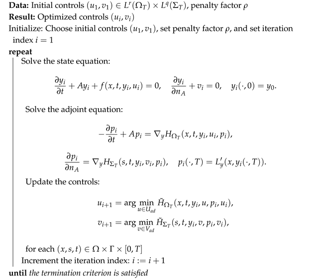3.4. Convergence of Algorithm

We now establish the convergence of Algorithm 2 through the following theorem.

Theorem 2. 

Suppose Assumptions 1 and 2 hold, and let $u_0\in \mathcal{U}$ and $v_0\in \mathcal{V}$ be any initial measurable controls satisfying $J(u_0,v_0)<+\infty$. Further, assume that ${inf}_{(u,v)\in \mathcal{U}\times \mathcal{V}}J(u,v)>-\infty$. Then, for $\rho >\tilde{C}$, if $u_i$ and $v_i$ are generated by Algorithm 2, there exist $\tilde{u}\in \mathcal{U}$ and $\tilde{v}\in \mathcal{V}$ such that

$$u_k\to \tilde{u}\mathrm{in}{L}^2\left({\Omega }_T\right)\mathrm{and}{v}_k\to \tilde{v}\mathrm{in}{L}^2\left({\Sigma }_T\right).$$

Proof. 

According to Lemma 3, we have

$$\begin{array}{cc}\hfill & J(u_{i+1},v_{i+1})-J(u_i,v_i)\le {\int }_{{\Omega }_T}[H_{{\Omega }_T}(y_i,u_{i+1})-H_{{\Omega }_T}(y_i,u_i)]dxdt\hfill \\ \hfill & +{\int }_{{\Sigma }_T}[H_{{\Sigma }_T}(y_i,v_{i+1})-H_{{\Sigma }_T}(y_i,v_i)]dsdt\hfill \\ \hfill & +\tilde{C}\left(\Vert u_{i+1}-u_i{\Vert }_{L^2\left({\Omega }_T\right)}^2+{\Vert v_{i+1}-v_i\Vert }_{L^2\left({\Sigma }_T\right)}^2\right).\hfill \end{array}$$

From the augmented Hamiltonian minimization step of Algorithm 2, we obtain

$$\begin{array}{c}\hfill H_{{\Omega }_T}(y_i,u_{i+1})+\rho {(u_{i+1}-u_i)}^2\le H_{{\Omega }_T}(y_i,u_i),\end{array}$$

$$\begin{array}{c}\hfill H_{{\Sigma }_T}(y_i,v_{i+1})+\rho {(v_{i+1}-v_i)}^2\le H_{{\Sigma }_T}(y_i,v_i),\end{array}$$

which implies

$$\begin{array}{cc}\hfill & J(u_{i+1},v_{i+1})-J(u_i,v_i)\hfill \\ \hfill & \le (\tilde{C}-\rho )\left(\Vert u_{i+1}-u_i{\Vert }_{L^2\left({\Omega }_T\right)}^2+{\Vert v_{i+1}-v_i\Vert }_{L^2\left({\Sigma }_T\right)}^2\right).\hfill \end{array}$$

Summing N terms under the condition $\rho >\tilde{C}$, we derive the following estimate

$$\begin{array}{cc}\hfill 0& \le \sum _{i=0}^N\left(\Vert u_{i+1}-u_i{\Vert }_{L^2\left({\Omega }_T\right)}^2+{\Vert v_{i+1}-v_i\Vert }_{L^2\left({\Sigma }_T\right)}^2\right)\hfill \\ \hfill & \le (\rho -\tilde{C})\left(J(u_0,v_0)-J(u_N,v_N)\right)\hfill \\ \hfill & \le (\rho -\tilde{C})\left(J(u_0,v_0)-\underset{(u,v)\in \mathcal{U}\times \mathcal{V}}{inf}J(u,v)\right).\hfill \end{array}$$

Thus, we have

$$\sum _{i=0}^{\infty }\left(\parallel u_{i+1}-u_i{\parallel }_{L^2\left({\Omega }_T\right)}^2+{\parallel v_{i+1}-v_i\parallel }_{L^2\left({\Sigma }_T\right)}^2\right)<+\infty .$$

By the Cauchy convergence criterion, there exist $\tilde{u}\in \mathcal{U}$ and $\tilde{v}\in \mathcal{V}$ such that $u_i\to \tilde{u}$ in $L^2\left({\Omega }_T\right)$ and $v_i\to \tilde{v}$ in $L^2\left({\Sigma }_T\right)$. □

4. Numerical Tests

In this section, we present numerical results for an optimal control problem governed by a parabolic partial differential equation defined on a two-dimensional domain $\Omega$. Problem (1) is solved using the Augmented Method of Successive Approximations (AMSA), as described in Algorithm 2. For comparison purposes, the Interior Point Method (IPM) and the Configuration Method (CM) are also implemented to solve the same problem. The numerical performance of these methods is compared to demonstrate the effectiveness and efficiency of the proposed AMSA.

All algorithms were implemented in Python 3.9.13. The numerical experiments were carried out on a desktop computer equipped with an Intel(R) Xeon(R) W-2245 CPU @ 3.90 GHz. Unless otherwise stated, all experiments were conducted under the same computational conditions.

The termination condition for the algorithm is given by

$$J\left(u_{i+1}\right)-J\left(u_i\right)<ϵ.$$

We consider the following optimal control problem with ${\Omega }_T=[0,1]\times [0,1]\times [0,1]$:

$$minJ(y,u):={\displaystyle \frac{1}{2}}\parallel y(·,T)-y_d{\parallel }_{L^2(\Omega )}^2+{\displaystyle \frac{\alpha }{2}}{\parallel u\parallel }_{L^2\left({\Omega }_T\right)}^2,$$

subject to

$$\left\{\begin{array}{cc}{y}_t-\Delta y=u+y,\hfill & \mathrm{in}{\Omega }_T,\hfill \\ {\partial }_{{\nu }_A}y=0,\hfill & \mathrm{on}{\Sigma }_T,\hfill \\ y(·,0)=y_0,\hfill & \mathrm{in}\overline{\Omega }.\hfill \end{array}\right.$$

Here, we choose the following parameters: $u_0=0.001$, $y_0=sin\left(\pi x\right)sin\left(\pi y\right)$, $y_d=exp(-2\alpha \pi T)sin\left(\pi x\right)sin\left(\pi y\right)$, $\alpha =1$, and $\rho =10$.

To solve the state and adjoint equations, we employ the finite difference method. The spatial step size is set to $0.01$ in each direction, and the time step size is set to $0.025$. The learning rate of gradient descent in the subproblem is dynamically adjusted, starting from $0.01$ and multiplying by $0.9$ if the change is not reduced and $1.1$ if the change is reduced. The termination criterion is set to $ϵ={10}^{-6}$. The numerical results obtained are presented below.

In order to evaluate the scalability of the proposed algorithm, Table 1 reports the computational time and maximum memory usage for solving the aforementioned example under varying temporal and spatial discretizations. Specifically, different time step sizes and spatial mesh resolutions are considered to assess the algorithm’s performance with respect to computational efficiency and memory consumption.

Table 1. Computation time and maximum memory usage of the proposed algorithm under different temporal and spatial discretizations.

Time Step Size	Space Step Size	Computation Time (s)	Maximum Memory Usage (MB)
0.1	0.1	0.4888	68.09
0.05	0.05	0.6886	69.15
0.025	0.025	17.4842	75.84
0.0125	0.0125	170.6029	116.42

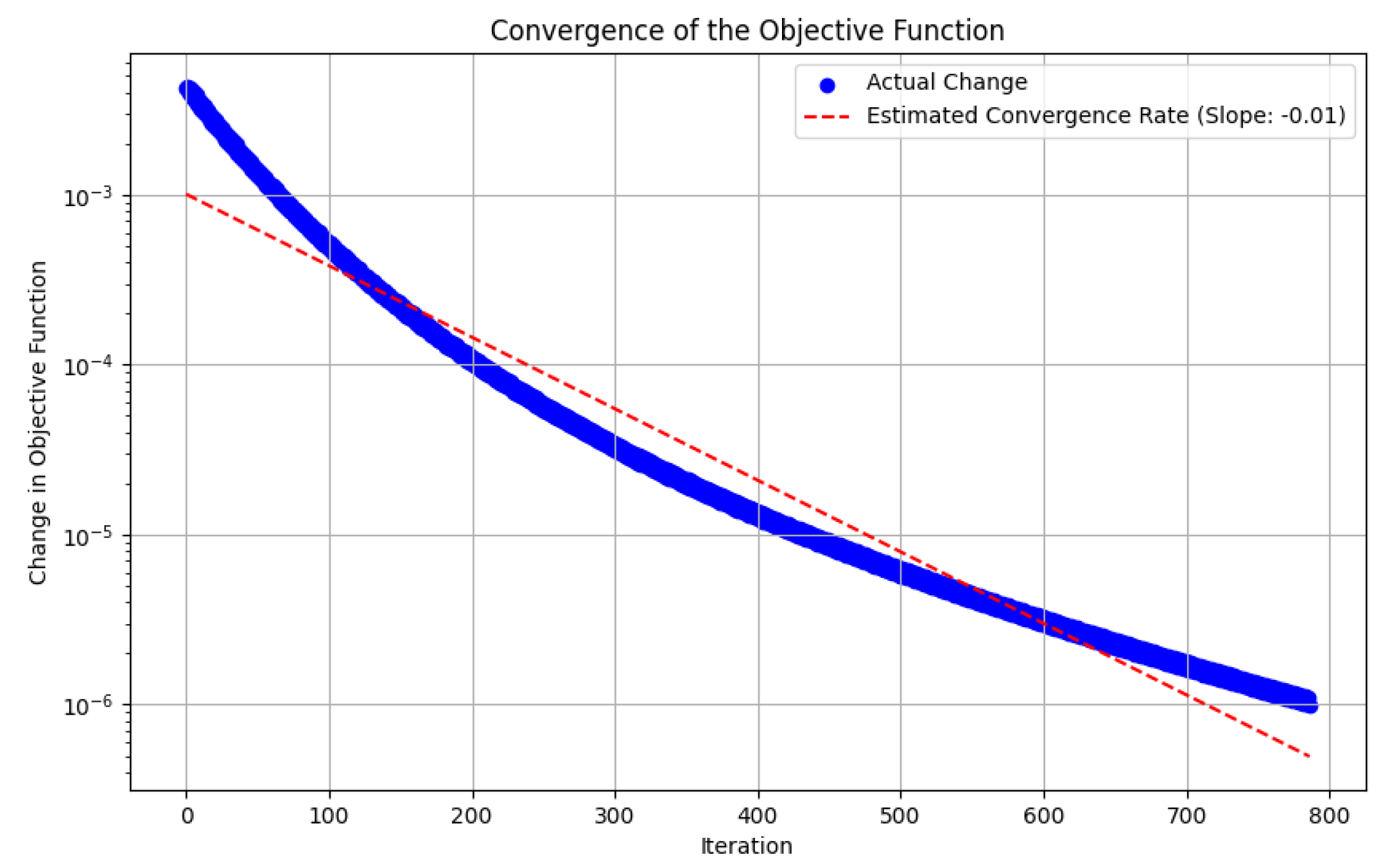
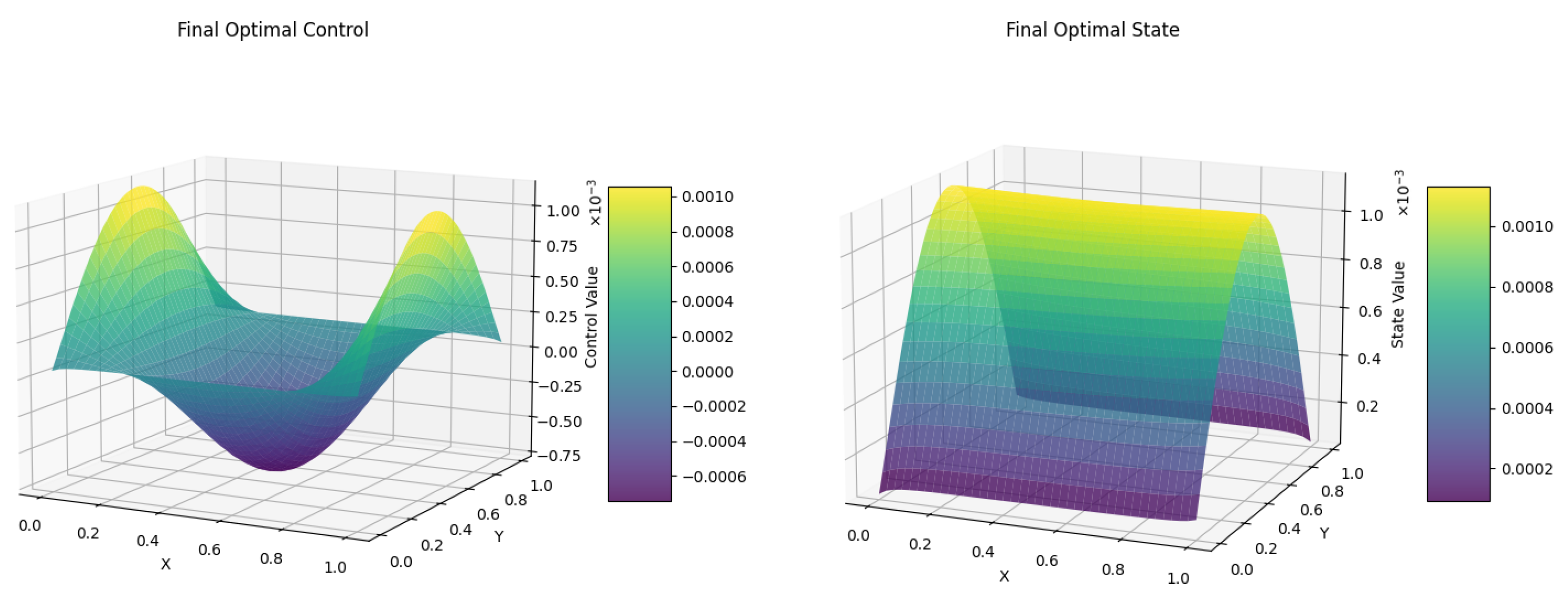
As shown in Figure 1, the difference in objective function values generally exhibits a monotonically decreasing trend, which demonstrates the effectiveness of the proposed Augmented Method of Successive Approximations (AMSA). Figure 2 presents the numerically obtained optimal control u and the corresponding optimal state y. It is noted that, since a gradient descent method is employed to solve the Hamiltonian optimization subproblem, the algorithm may converge to a local optimal solution. The robustness and solution quality can be further enhanced by employing stochastic gradient descent, multi-start strategies, adaptive learning rate schemes, or by integrating global optimization techniques. These approaches have the potential to effectively mitigate the aforementioned limitation.

Figure 1. Difference in Objective Function $J\left(u_{i+1}\right)$−$J\left(u_i\right)$ via AMSA(GD).

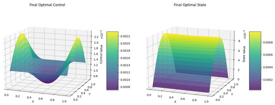
Figure 2. Computed optimal state y (right) and optimal control u (left) via AMSA(GD).

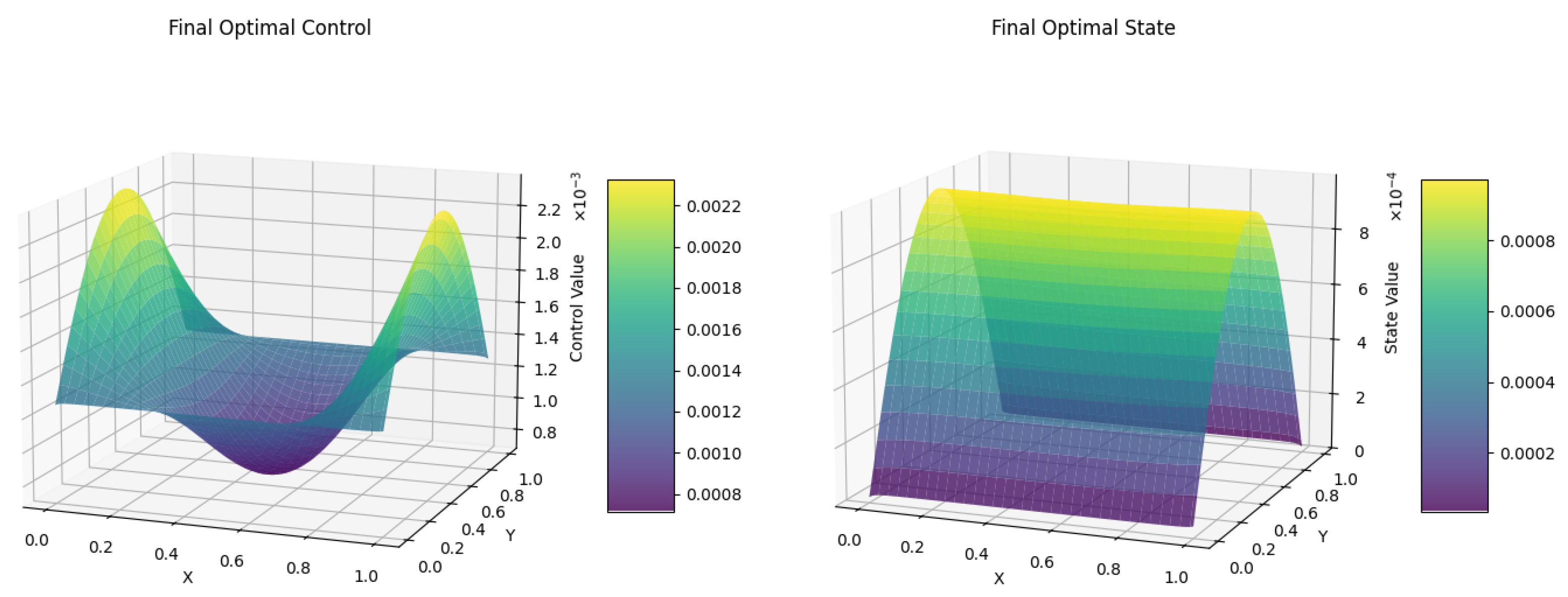
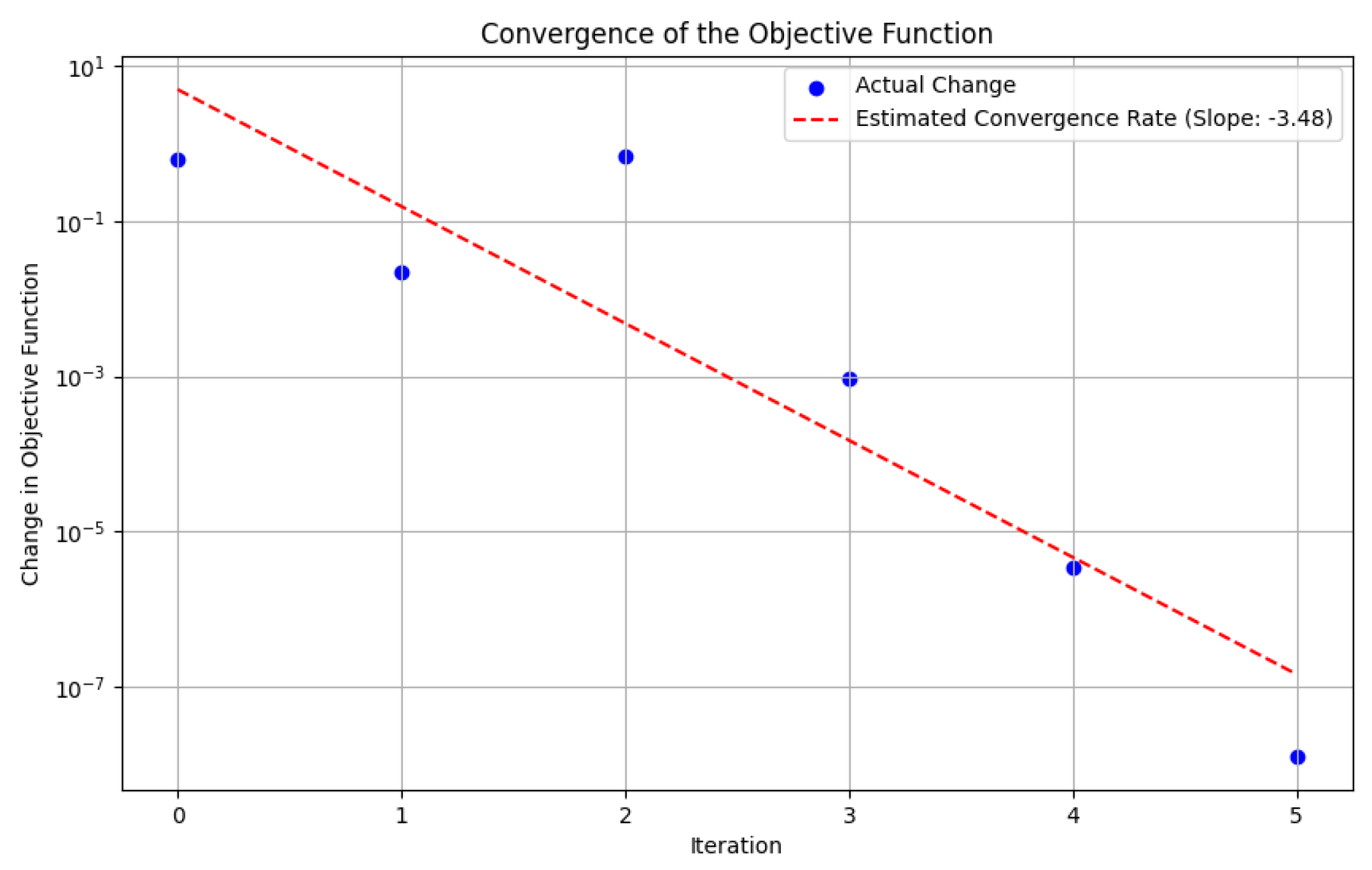
To further investigate this possibility, we replace the gradient descent method in the Hamiltonian optimization step with the Simulated Annealing (SA) algorithm. In this case, the initial temperature is set to 100, and the cooling rate is set to $0.95$. The temporal and spatial discretization steps are both fixed at $0.025$. The corresponding numerical results are presented as follows. Figure 3 illustrates the difference in the objective function obtained using the AMSA (SA) method. Figure 4 presents the optimal control u derived from this method, along with the corresponding optimal state y.

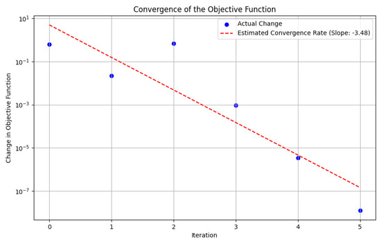
Figure 3. Difference in Objective Function $J\left(u_{i+1}\right)$−$J\left(u_i\right)$ via AMSA(SA).

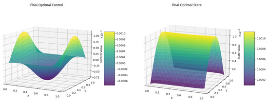
Figure 4. Computed optimal state y (right) and optimal control u (left) via AMSA(SA).

Table 2 reports the computation time, maximum memory usage, and the optimal objective function value obtained when employing the gradient descent (GD) algorithm and the Simulated Annealing (SA) algorithm to solve the augmented Hamiltonian subproblem. In this experiment, both the time step size and the space step size are fixed at $0.025$.

Table 2. Comparison of computation time, maximum memory usage, and optimal objective function value using GD and SA algorithms for the augmented Hamiltonian subproblem. The time step size and space step size are both set to $0.025$.

Method	Computation Time (s)	Maximum Memory Usage (MB)	Objective Function J
GD	17.4842	75.84	0.00105496
SA	0.3079	75.95	0.00033848

As shown in Table 2, the SA method avoids convergence to a local optimum and achieves a superior optimal objective function value compared to the GD method. In addition, the computation time of SA is significantly reduced, while the maximum memory usage remains similar.

Furthermore, we compare the optimal objective function values, computation time, and maximum memory usage of the Interior Point Method (IPM), Configuration Method (CM), and the proposed AMSA (implemented with SA) under the same discretization parameters. Specifically, the time step size and space step size are both set to 0.05. The corresponding numerical results are summarized in Table 3.

Table 3. Comparison of IPM, CM, and AMSA (with SA) in terms of computation time, maximum memory usage, and optimal objective function value. The time step size and space step size are both set to $0.05$.

Method	Computation Time (s)	Maximum Memory Usage (MB)	Objective Function J
IPM	54.7279	1392.05	0.00055791
CM	2.5713	128.82	0.00401861
AMSA (SA)	0.0206	68.64	0.00195774

From Table 3, it can be observed that AMSA exhibits significantly lower computation time and memory consumption compared to IPM and CM for the same time and space step sizes. However, the optimal objective function value obtained by AMSA is inferior to that of IPM. By combining the observations from Table 2 and Table 3, it can be concluded that AMSA is capable of obtaining an optimal solution superior to IPM when finer discretization (smaller time and space step sizes) is employed. Despite the improved solution quality, AMSA still maintains much lower computation time and memory usage than IPM, highlighting its effectiveness and computational efficiency.

5. Discussion

Based on the work presented in [21], the AMSA algorithm is applied to the optimal control problem of a class of parabolic equations, for which a rigorous convergence proof has been provided. This framework facilitates the integration of more sophisticated deep learning algorithms that are capable of decoupling and iteratively updating the parameters of each layer.

Moreover, by incorporating global optimization algorithms into the solution process of the augmented Hamiltonian subproblem, the issue of convergence to a local optimal solution can be effectively mitigated. Future work will focus on the development of second-order convergence algorithms with accelerated convergence rates. The goal is to solve the augmented Hamiltonian maximization subproblem more efficiently and robustly, ensuring both the convergence quality and computational efficiency of the overall method.

References

- Bardi, M.; Capuzzo-Dolcetta, I. Optimal Control and Viscosity Solutions of Hamilton-Jacobi-Bellman Equations; With Appendices by Maurizio Falcone and Pierpaolo Soravia; Systems & Control: Foundations & Applications; Birkhäuser Boston, Inc.: Boston, MA, USA, 1997; p. xviii+570. [Google Scholar] [CrossRef]
- Falcone, M.; Ferretti, R. Semi-Lagrangian Approximation Schemes for Linear and Hamilton-Jacobi Equations; Society for Industrial and Applied Mathematics (SIAM): Philadelphia, PA, USA, 2014; p. xii+319. [Google Scholar]
- Casas, E. Pontryagin’s principle for state-constrained boundary control problems of semilinear parabolic equations. SIAM J. Control Optim. 1997, 35, 1297–1327. [Google Scholar] [CrossRef]
- Raymond, J.P.; Zidani, H. Hamiltonian Pontryagin’s principles for control problems governed by semilinear parabolic equations. Appl. Math. Optim. 1999, 39, 143–177. [Google Scholar] [CrossRef]
- Kang, W.; Wilcox, L.C. Mitigating the curse of dimensionality: Sparse grid characteristics method for optimal feedback control and HJB equations. Comput. Optim. Appl. 2017, 68, 289–315. [Google Scholar] [CrossRef]
- Stefansson, E.; Leong, Y.P. Sequential alternating least squares for solving high dimensional linear Hamilton-Jacobi-Bellman equation. In Proceedings of the 2016 IEEE/RSJ International Conference on Intelligent Robots and Systems (IROS), Daejeon, Republic of Korea, 9–14 October 2016; pp. 3757–3764. [Google Scholar] [CrossRef]
- Beard, R.W.; Saridis, G.N.; Wen, J.T. Galerkin approximations of the generalized Hamilton-Jacobi-Bellman equation. Automatica J. IFAC 1997, 33, 2159–2177. [Google Scholar] [CrossRef]
- Beard, R.W.; Saridis, G.N.; Wen, J.T. Approximate solutions to the time-invariant Hamilton-Jacobi-Bellman equation. J. Optim. Theory Appl. 1998, 96, 589–626. [Google Scholar] [CrossRef]
- Beeler, S.C.; Tran, H.T.; Banks, H.T. Feedback control methodologies for nonlinear systems. J. Optim. Theory Appl. 2000, 107, 1–33. [Google Scholar] [CrossRef]
- Kalise, D.; Kunisch, K. Polynomial approximation of high-dimensional Hamilton-Jacobi-Bellman equations and applications to feedback control of semilinear parabolic PDEs. SIAM J. Sci. Comput. 2018, 40, A629–A652. [Google Scholar] [CrossRef]
- Alla, A.; Falcone, M.; Kalise, D. An efficient policy iteration algorithm for dynamic programming equations. SIAM J. Sci. Comput. 2015, 37, A181–A200. [Google Scholar] [CrossRef]
- Bokanowski, O.; Maroso, S.; Zidani, H. Some convergence results for Howard’s algorithm. SIAM J. Numer. Anal. 2009, 47, 3001–3026. [Google Scholar] [CrossRef]
- Howard, R.A. Dynamic Programming and Markov Processes; Technology Press of M.I.T.: Cambridge, MA, USA; John Wiley & Sons, Inc.: New York, NY, USA; London, UK, 1960; p. viii+136. [Google Scholar]
- Bryson, A.E., Jr.; Ho, Y.C. Applied Optimal Control: Optimization, Estimation, and Control; Revised Printing; Hemisphere Publishing Corp.: Washington, DC, USA; Distributed by Halsted Press [John Wiley & Sons, Inc.]: New York, NY, USA; London, UK; Sydney, Australia, 1975; p. xiv+481. [Google Scholar]
- Roberts, S.M.; Shipman, J.S. Two-point boundary value problems: Shooting methods. In Modern Analytic and Computational Methods in Science and Mathematics; American Elsevier Publishing Co., Inc.: New York, NY, USA, 1972; Volume 31, p. xiv+277. [Google Scholar]
- Betts, J.T.; Frank, P.D. A sparse nonlinear optimization algorithm. J. Optim. Theory Appl. 1994, 82, 519–541. [Google Scholar] [CrossRef]
- Betts, J.T. Experience with a sparse nonlinear programming algorithm. In Large-Scale Optimization with Applications, Part II (Minneapolis, MN, 1995); Springer: New York, NY, USA, 1997; Volume 93, pp. 53–72. [Google Scholar] [CrossRef]
- Bertsekas, D.P. Nonlinear Programming, 2nd ed.; Athena Scientific Optimization and Computation Series; Athena Scientific: Belmont, MA, USA, 1999; p. xiv+777. [Google Scholar]
- Bazaraa, M.S.; Sherali, H.D.; Shetty, C.M. Nonlinear Programming, 3rd ed.; Theory and Algorithms; Wiley-Interscience [John Wiley & Sons]: Hoboken, NJ, USA, 2006; p. xvi+853. [Google Scholar] [CrossRef]
- Chernous‘ko, F.L.; Lyubushin, A.A. Method of successive approximations for solution of optimal control problems. Optimal Control Appl. Methods 1982, 3, 101–114. [Google Scholar] [CrossRef]
- Li, Q.; Chen, L.; Tai, C. Maximum principle based algorithms for deep learning. J. Mach. Learn. Res. 2017, 18, 1–29. [Google Scholar]
- Hestenes, M.R. Multiplier and gradient methods. J. Optim. Theory Appl. 1969, 4, 303–320. [Google Scholar] [CrossRef]
- Sethi, D.; Šiška, D. The modified MSA, a gradient flow and convergence. Ann. Appl. Probab. 2024, 34, 4455–4492. [Google Scholar] [CrossRef]
- Aleksandrov, V.V. On the accumulation of perturbations in the linear systems with two coordinates. Vestn. MGU 1968, 3, 67–76. [Google Scholar]
Disclaimer/Publisher’s Note: The statements, opinions and data contained in all publications are solely those of the individual author(s) and contributor(s) and not of MDPI and/or the editor(s). MDPI and/or the editor(s) disclaim responsibility for any injury to people or property resulting from any ideas, methods, instructions or products referred to in the content. |
© 2025 by the authors. Licensee MDPI, Basel, Switzerland. This article is an open access article distributed under the terms and conditions of the Creative Commons Attribution (CC BY) license (https://creativecommons.org/licenses/by/4.0/).