A Hybrid Long Short-Term Memory-Graph Convolutional Network Model for Enhanced Stock Return Prediction: Integrating Temporal and Spatial Dependencies

Abstract

Stock return prediction is a pivotal yet intricate task in financial markets, challenged by volatility and multifaceted dependencies. This study proposes a hybrid model integrating long short-term memory (LSTM) networks and graph convolutional networks (GCNs) to enhance accuracy by capturing both temporal dynamics and spatial inter-stock relationships. Tested on the Dow Jones Industrial Average (DJIA), Shanghai Stock Exchange 50 (SSE50), and China Securities Index 100 (CSI 100), our LSTM-GCN model outperforms baselines—LSTM, GCN, RNN, GRU, BP, decision tree, and SVM—achieving the lowest mean squared error (e.g., 0.0055 on DJIA), mean absolute error, and highest R² values. This superior performance stems from the synergistic interaction of spatio-temporal features, offering a robust tool for investors and policymakers. Future enhancements could incorporate sentiment analysis and dynamic graph structures.

1. Introduction

Predicting stock returns is essential for investment strategies and economic policy but remains challenging due to market volatility, non-stationarity, and behavioral unpredictability. While deep learning, notably LSTM, excels at temporal modeling, it neglects inter-stock spatial relationships, which GCNs [1] effectively capture. Our hybrid LSTM-GCN model bridges this gap, aiming to improve forecasting accuracy by integrating these dimensions. We compare it against diverse baselines and discuss its implications for financial decision-making.

As an important component of the financial market, the stock market has attracted many people to invest. Knowing the movement of the stock can also help policy makers to have a better understanding of the development of the economy. Based on these reasons, the prediction of the stock price is always a hot topic for researchers. However, due to the high volatility of the stock and the irrational behavior of the investor, the forecast of stock prices is very hard. And the stock price movement is not always stationary which means the prediction of it has a lack of support in theory. Stock market prediction is vital for investors seeking profitable opportunities and policymakers analyzing economic trends. However, the task is complicated by market volatility, non-stationarity, and irrational investor behavior. Traditional statistical models struggle with these dynamics due to restrictive assumptions, while deep learning offers a promising alternative. Long short-term memory (LSTM) networks excel at modeling temporal dependencies in time series data, yet they overlook the spatial relationships among stocks. Graph convolutional networks (GCNs) address this gap by capturing topological structures [1].

With the development of the technology, deep learning is becoming more and more popular in research due to its positive performance in prediction. It is reasonable to apply neural networks in research for stock return prediction. Because LSTM is a common cyclic neural network, it has been widely used in the modeling and prediction of time series data. With the advantage of memorizing the long-term information and analyzing the structure of the data, LSTM can predict the future return of the stocks and provide valuable information for investors by learning the historical stock price.

However, the single long short-term memory neural network can only capture the long-term dependence relationship without finding the topology relationship existing in the stock market. So, as a new model which is good at processing the figure structure data and extracting topology information, the graph neural network is used to capture the nonlinear relationship and complex network structure in the stock market. Graph convolution networks [1] aim to effectively learn the representation of graph structure data and achieve high-quality node classification. By transforming the stocks to points and their relationship into a line on the graph, GCN can effectively analyze the association between different stocks and capture the potential factors, to improve the prediction accuracy of stock yields.

By combining these two networks, the proposed model can not only capture the time factors which have been important in the previous research, but also can find the spatial information through the graph structure composed by stock and relationship. More importantly, the proposed model can also realize the interaction of time information and space information to obtain a more accurate prediction.

In this paper, we will discuss how to combine the LSTM and GCN to predict the returns on the stock. And then, we compare the performance of the proposed model with other basic models, like GCN, LSTM, and linear regression, to analyze and evaluate the performance of the model, and discuss possible improvements and future research directions. Through the research of this article, we hope to provide new ideas and methods for financial market forecasting and provide investors with more accurate decision-making support. We propose a hybrid LSTM-GCN model that synergistically combines temporal and spatial information to predict stock returns. We evaluate its performance against baseline models (e.g., LSTM, GCN, linear regression) using real-world datasets and explore its advantages and limitations. Our contribution enhances financial forecasting methodologies, empowering stakeholders with more accurate decision-making tools.

2. Related Work

Traditional ‘model-driven’ methods like ARMA [2] and GARCH [3] assume stationarity and linear relationships, limiting their effectiveness in volatile markets [4]. Deep learning has shifted the focus to ‘data-driven’ approaches. Pramod and Pm (2021) [5] utilized LSTM for stock price prediction, while Darapaneni et al. (2022) [6] enhanced it with sentiment analysis, though both struggled with non-stationary price data. Qiu et al. (2020) [7] introduced attention mechanisms to LSTM, improving feature focus, yet spatial dependencies remained unaddressed.

Graph-based models have tackled spatial structures. Son and Kim (2019) [8] proposed a graph-based asset pricing model, and Zhang and Wei (2019) [9] applied GNNs to financial time series. Shi and Meng (2020) [10] combined GCN and LSTM but fell short of fully integrating spatio-temporal interactions. Meng and Wang (2021) [11] advanced this with dynamic GCNs, adapting to evolving relationships, while Liu et al.’s (2020) [12] SCINet improved temporal resolution but ignored spatial context.

Despite these advances, the following key challenges persist: (1) capturing evolving inter-stock relationships over time, (2) integrating exogenous factors (e.g., sentiment, macroeconomic indicators) into spatio-temporal models, (3) addressing overfitting in complex hybrid architectures, and (4) ensuring scalability across diverse markets. Our LSTM-GCN model addresses the first by enabling spatio-temporal interaction, setting the stage for tackling the remaining issues in future work.

The previous researchers have always used ‘model-driven’ methods to predict the return of stocks. The autoregressive moving average model, proposed by Box and Jenkins [2], is widely used in the analysis of time series data, especially in the field of economic and financial data analysis. The ARMA model assumes that the time series is stationary, so it is usually necessary to differentially process the non-stationary sequence before applying the model to turn it into a stationary sequence. Engle, R.F. [3] introduced the ARCH model, which is crucial for modeling financial time series that exhibit time-varying volatility, a precursor to the GARCH models. The generalized autoregressive conditional heteroskedasticity model, proposed by Bollerslev [4], can better capture the fluctuation aggregation phenomenon of financial time series. Sims [13] proposed the VAR model which is a multivariate time series model that can predict the future values of multiple interdependent time series data at the same time. But these models have serious assumptions that limit the performance of the models.

With the development of the deep learning algorithm, the ‘data-driven’ method is becoming popular. Due to the limited needs of some strong assumptions and their ability to simulate other functions, many prediction studies have contained this method. Pramod [5] predicted the movement of the stock price using LSTM. Narayana Darapaneni [6] explored stock price prediction using LSTM and sentiment analysis. They incorporated historical prices and sentiment data into their models, which included LSTM and random forest, to predict stock prices of specific companies. Hao PY [14] extracted emotional information and then analyzed the stock trend based on support vector machine. Adhikari [15] proposed a hybrid deep learning model for stock price prediction that utilized sentiment analysis to enhance prediction accuracy compared to traditional methods. Kabadi [16] discussed a hybrid approach that uses prediction rule ensembles (PREs) and deep neural networks (DNNs) for stock price prediction. Chandar S K [17] used a hybrid model based on artificial neural networks to forecast the stock price. Zhao J [18] used a recurrent neural network to predict stock prices. Firuz Kamalov [19] summarized the deep learning method used on the stock price forecast on the S&P 500. Qiu [7] forecasted stock prices with a long-short term memory neural network based on attention mechanism on the DJIA, HIS, and S&P 500. But these research studies have mainly focused on the prediction of a stock price which is not stationary, and that has a lack of support in theory.

Traditional neural networks can capture the key time information contained in the data while some information hides in the relationship between components. To solve this problem, there are already some researchers using other versions of perceptron to analyze the spatial structure of the data. Hamilton, J.D. [20] developed state–space models which are also vital for capturing latent structures in time series, providing a method to account for shifts and trends that are not observable directly. Son [8] proposed a new asset pricing model based on a graph structure before that graph-based model is always used in image processing. They set the covariance between different assets as the adjacent matrix and the assets’ price as the points in the graph. Liu [12] proposed SCINet which employs a novel architecture that combines down sampling and convolution operations to capture both local and global views of time series data. This allows for effective feature learning across different temporal resolutions, enhancing the model’s ability to forecast based on comprehensive time-dependent information. Zhang [9] attempted to use a graph neural network to perform financial time series analysis. Shi [10] applied a GCN-LSTM neural network to predict the stock price. Although this paper also uses the combination of the graph and LSTM, it does not realize the interaction of the time and spatial information. Meng, Q. [11] developed a dynamic graph convolutional network that updates the graph structure over time, allowing for the modeling of evolving relationships in financial markets. My model advances these works by explicitly capturing the interaction between the temporal and spatial information in the stock market. While previous models, like those proposed by Shi and Meng, have leveraged the combination of GCN and LSTM or dynamic graph convolution, they often do not fully exploit the interaction between temporal and spatial information. My approach ensures that both the temporal dependencies and the topological relationships between stocks are considered simultaneously. This allows for a more comprehensive and accurate understanding of stock price movements. Furthermore, unlike SCINet which primarily focuses on temporal resolutions, my model integrates both time-dependent and spatial features directly, leading to improved prediction accuracy and robustness. This holistic approach to financial market forecasting provides a more precise methodology, advancing the field by ensuring that evolving relationships and time-dependent patterns are captured together.

The following sections delve into our core methodology and findings. Section 3 reviews traditional models like LSTM and GCN, then details our proposed LSTM-GCN network, highlighting its design, principles, and advantages. Section 4 validates our model’s effectiveness through empirical experiments, describing datasets, experimental setups, and evaluation metrics, with performance comparisons to baseline models. Section 5 summarizes key findings, discusses the contributions of our LSTM-GCN model to stock return prediction, and suggests future research directions.

3. Method

3.1. Basis of Our Method

3.1.1. LSTM

Long short-term memory (LSTM) networks are a special kind of recurrent neural network (RNN) capable of learning long-term dependencies, a common issue in traditional RNNs. There are three gates in each perceptron of LSTM which are the input gate, the forget gate, and the output gate. The data come to this system through the input gate. Then, this system extracts useful information through linear combination and non-linear activating to match the real situation. The valuable information is packaged into hidden status and is delivered to the next perceptron through the output gate. The forget gate choses what information should be considered in this cell and exclude the information needed to be forgotten. The sigmoid and tanh function is always considered to be the active function to add non-linear information to the system. And the existence of the hidden status allow LSTM memory the information before. Combined with the new information, LSTM can have a better prediction compared with traditional RNN. LSTM networks mitigate vanishing gradients in RNNs via input, forget, and output gates, adeptly modeling long-term temporal dependencies in stock return sequences.

3.1.2. GCN

Unlike LSTM which extracts time information, graph convolutional network is used to extract the spatial information according to the structure of the assets which is represented by the correlation of these stocks. The key to operating GCNs is the definition of the graph whose components are the points and edges. I define the asset as dots with return calculated by the close price of each stock as the value of the point. In addition, the edge of the graph is defined by the correlation of each stock, if the correlation of a pair of stocks means there is an edge between these two stocks. But what should be considered is the effect of the market due to the situation that the market will increase the correlation of stocks that lead to a false high correlation of a pair of stocks. The extraction of the spatial information can be seen as a convolution process which means each node updates its value by applying a weighted average to its neighbors to aggregate information. In the average process, it is important to normalize each node according to its degrees to ensure that nodes contribute equally to the aggregation process.

So, the process of the updating of GCNs can be expressed as follows:

$$F_{l+1}=\sigma \left({\tilde{S}}^{-{\displaystyle \frac{1}{2}}}\tilde{A}{\tilde{S}}^{-{\displaystyle \frac{1}{2}}}{F}_l{W}_l\right)$$

(1)

where $F_l$ represents the feature matrix at layer $l;\tilde{A}$ is the adjacency matrix with added self-connection; $\tilde{s}$ is the degree matrix of $\tilde{A}$ and used to normalize the adjacency matrix; $W_l$ is the weight matrix for layer $l$; and $\sigma$ is a non-linear activation function.

GCNs process graph-structured data, representing stocks as nodes and their correlations (threshold: 0.3, validated via cross-validation) as edges. The convolution aggregates neighbor information:

$$H^{l+1}=\sigma \left({\tilde{D}}^{-1/2}\tilde{A}{\tilde{D}}^{-1/2}{H}^{\left(l\right)}{W}^{\left(l\right)}\right)$$

where $\tilde{A}$ includes self-loops; $\tilde{D}$ normalizes by degree; and $\sigma$ (e.g., ReLU) adds non-linearity [1].

3.2. Proposed Method—LSTM-GCN

3.2.1. The Idea

The mean work of this study is to combine long short-term memory networks and graph convolutional networks to forecast real world date’s returns. The strength of the proposed model can be divided into two dimensions.

For the temporal dimension, the LSTM can use new information combined with the previous information to make a prediction or extract the time factors just like the statement in Section 3.1.1.

Combined with the temporal analysis, GCNs are employed to add new information into the system by analyzing the relationship between stocks. The cut-off that is used to define whether there is an edge is 0.3 which is chosen by cross validation method as a range of cut-off is settled to a repeatable experiment. Then, the best result of experiments with different cut-offs are displayed in this paper.

The transmission process of information is an interaction process of the perceptron of GCNs and LSTMs. Through this interaction, this system can not only capture the trend of the stock but also capture the effect from other stocks. So, the proposed model is expected to produce a more robust and accuracy prediction result compared with those models only using one type of information.

3.2.2. Process

First, to remove the effect of the common pattern, PCAs are employed to remove it from the first order difference in the price.

After obtaining the return with no common pattern, to capture long-term dependencies in the series data, the LSTM network was used to process the time series data of 30 stocks. Each LSTM neuron can learn the time patterns in stock returns by extracting time-related information from stock earnings data, retaining those important time features. After the LSTM layer processes the time series data, a GCN will be employed to each LSTM’s hidden status to capture the spatial information from the stocks.

After being processed by the GCN layer, the hidden status contains spatio-temporal information and will be input into the next LSTM layer. By repeating this process, the hidden status is delivered from previous nodes to future nodes. Therefore, the combined information flows in this system.

Finally, the output from the last GCN layer will be used to predict index returns. These final results of this system take into consideration both time and structure information, which is a solid forecast for index returns.

This hybrid LSTM-GCN method combines the advantages of two types of neural networks and can effectively capture complex dynamics in stock returns. The process is as follows:

• Preprocessing: PCA removes market-wide effects from return series;
• LSTM Layer: Extracts temporal patterns from 30-stock sequences;
• GCN Layer: Enriches hidden states with spatial relationships;
• Iteration: Stacked layers propagate integrated features;
• Output: Final GCN layer predicts index returns.

3.2.3. Key Algorithms

Algorithm 1 outlines the core procedure of the LSTM-GCN model for stock return prediction. It initializes the input data and then iteratively processes the data through stacked LSTM and GCN layers to obtain the result.

Algorithm 1: LSTM-GCN Combined Network for Stock Return Prediction

Input: X: Input feature matrix of shape (num_stocks, time_steps, features) A: Adjacency matrix representing the connections between stocks W_lstm: Weight matrices for LSTM layers W_gcn: Weight matrices for GCN layers num_layers: Number of LSTM-GCN layers to stack Output: y_pred: Predicted index return 1:  function LSTM_GCN_Network(X, A, W_lstm, W_gcn, num_layers): 2:   Step 1: Initial input to the network 3:   Initialize H as X 4:   for layer in range(num_layers): 5:     Step 2: LSTM Layer 6:     H_lstm = LSTM_Layer(H, W_lstm[layer]) 7: 8:     Step 3: GCN Layer 9:     H_gcn = GCN_Layer(A, H_lstm, W_gcn[layer]) 10: 11:    Step 4: Update H for the next iteration 12:    H = H_gcn 13: 14:   Step 5: Final LSTM Layer to obtain the prediction 15:   y_pred = LSTM_Layer(H, W_lstm[num_layers]) 16: 17:   return y_pred

3.2.4. Complexity Analysis

The complexity of the LSTM layer is determined by the length of the sequence T, the dimension of input vector in LSTM as F_i,n, and the hidden status’ dimension H. At each time step, the LSTM layer executes a series of matrix multiplications and nonlinear activations. So the computation complex of LSTM can be expressed as $O(T\ast F_{i,n}\ast H)$ which is related to the sample size. In other words, as the length of the input sequence increases, the calculation time of LSTM will also increase.

The complexity of the GCN layer is determined by the dimension of adjacency matrix A and the dimension of the hidden state H from previous LSTM layer. The key operation in a GCN layer is the matrix multiplication between the adjacency matrix and the feature matrix. So, the computation time complex of the GCN layer can be expressed as $O(N^2\ast H)$.

The total complexity for N LSTM-GCN layers is obtained by summing the complexities of the individual LSTM and GCN layers and then multiplying by the number of layers. This can be expressed as: $O\left(N_{layers}\right(T\ast H+\ast H\left)\right)$

4. Experiment

4.1. Data

We used daily closing prices from 30 DJIA stocks and the DJIA index, sourced from Yahoo Finance (4 March 2021–4 March 2022), alongside SSE50 and CSI 100 datasets for validation (same period). Each dataset includes N = 30 stocks, T = 252 trading days, and features (returns). Training (80%) and test (20%) sets were split chronologically.

Table 1. The details of the data.

Date	AAPL	AXP	BA	…	WMT	XOM	Index
4 March 2021	118.0709	137.2385	224.710	…	40.5780	51.8341	30,924.14
5 March 2021	119.3388	141.7112	223.220	…	41.0839	53.7941	31,496.30
8 March 2021	114.3655	144.5390	224.030	…	40.6894	53.7411	31,802.44
9 March 2021	119.0144	139.5662	230.610	…	41.0107	52.9112	31,832.74
10 March 2021	117.9235	141.1533	245.340	…	42.0576	54.5357	32,297.02

exemplifies DJIA data (e.g., AAPL, AXP, BA, WMT, XOM). The dataset comprises daily returns of 30 individual stocks along with the corresponding DJIA index returns. Each row represents a particular date, and the columns include the stock price and the index price. The data span multiple days, providing a comprehensive view of the stock and index performance over time. It is collected from Yahoo Finance website. Daily closing prices for 30 DJIA stocks (e.g., AAPL, AXP, BA, WMT, XOM) and the DJIA index, plus SSE50 and CSI 100, were sourced from Yahoo Finance (4 March 2021–4 March 2022). Each dataset has N = 30 stocks, T = 252 days, and returns as features. An 80-20 chronological split separated training and test sets.

To support the results of the experiment, another two indexes were collected to repeat the experiment. They are Shanghai Stock Exchange 50 and China Securities Index 100 which are also collected from Yahoo Finance website.

4.2. Experimental Setup

The LSTM-GCN model comprises 2–4 stacked layers (tuned via grid search). Hyperparameters include the following:

• Learning Rate: 0.001;
• Batch Size: 32;
• Epochs: 200 (early stopping after 10 epochs without improvement);
• Optimizer: Adam;
• Loss: MSE;
• Initialization: Xavier.

Baseline models (LSTM, GCN, RNN, GRU, BP, Decision Tree, SVM) were similarly tuned (

Table 2. Model hyperparameters.

Model	Layers	Neurons/Layer	Learning Rate	Batch Size	Epochs
LSTM-GCN	3	64	0.001	32	200
LSTM	2	64	0.001	32	200
GCN	2	64	0.002	32	200
RNN	2	64	0.001	32	200
GRU	2	64	0.001	32	200
BP	3	128	0.01	64	100
Decision Tree	-	-	-	-	-
SVM	-	-	-	-	-

). Experiments were implemented in Python 3.8 using TensorFlow 2.5 and PyTorch 1.9. Hyperparameters were optimized via grid search over learning rates (0.0001–0.01) and layer counts (1–5), consistent across datasets.

4.3. Evaluation Metric

We used MSE, MAE, and R² as follows:

$$MSE={\displaystyle \frac{1}{n}}{\sum }_{i=1}^n{(y_i-\widehat{y_i})}^2$$

$$MAE={\displaystyle \frac{1}{n}}{\sum }_{i=1}^n|y_i-\widehat{y_i}|$$

$$R^2=1-{\displaystyle \frac{\frac{1}{n}{\sum }_{i=1}^n{(y_i-\widehat{y_i})}^2}{\frac{1}{n}{\sum }_{i=1}^n{(y_i-\overline{y})}^2}}$$

where $y_i$ is the actual return; $\widehat{y_i}$ is the predicted return; and $\overline{y}$ is the mean return.

4.4. Results

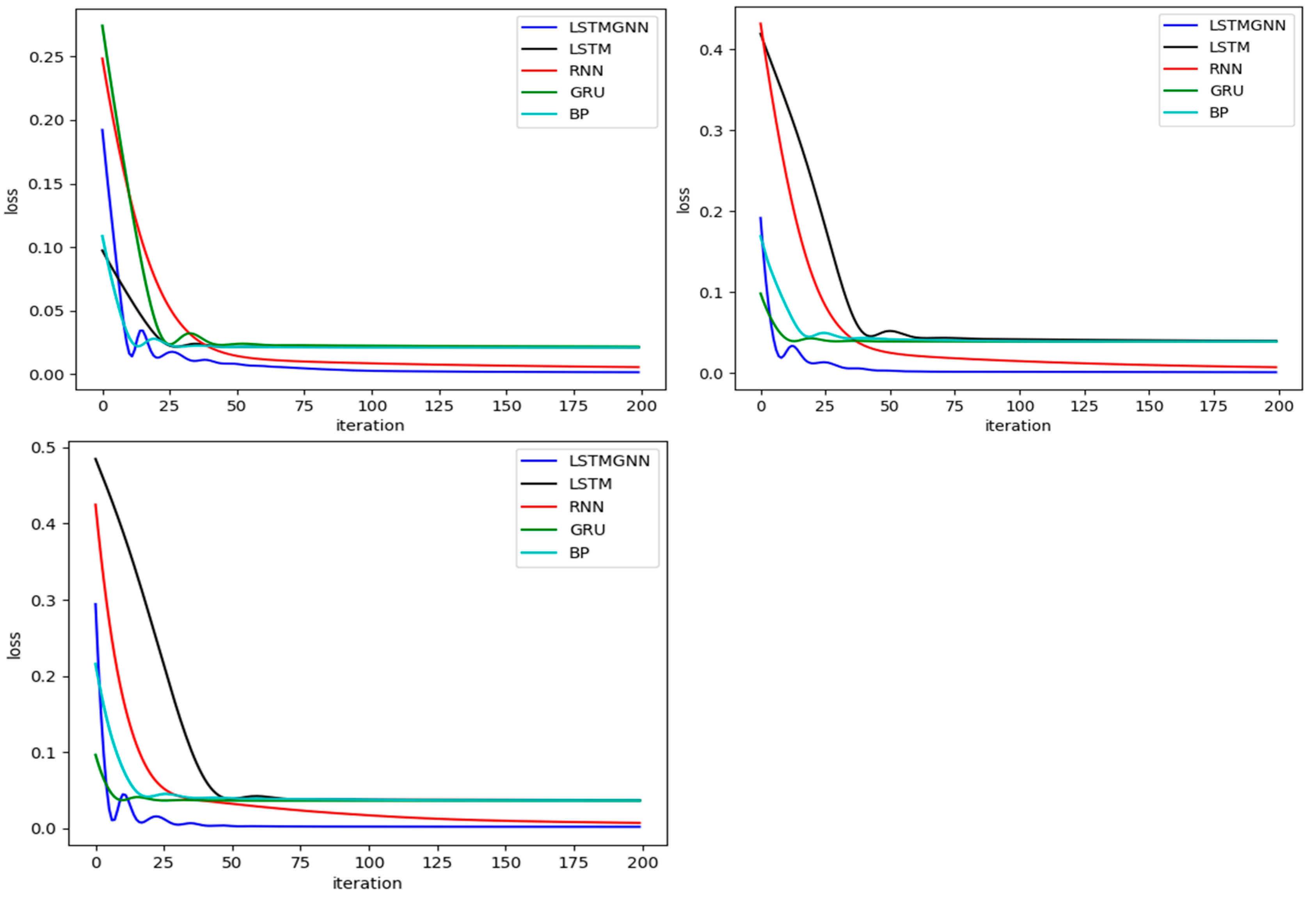
4.4.1. Iteration vs. Loss Function

After confirming the dataset had no abnormal valued and no missing values, the prices are processed to be the daily return of the stocks to make the time series become stationary. Then, the responding data are put into the computer environment to train the LSTM-GCN model. The dataset is divided into two parts, where 80% of the dataset is marked as training dataset and the other 20% of the dataset is the test dataset. There are another four neural networks which are also trained to make a comparison. The relative results of the three datasets of the training procedure are shown in Figure 1:

Training loss (MSE) decreased fastest for LSTM-GCN across all datasets (Figure 1), reflecting efficient spatio-temporal learning. Baseline models converged slower, with BP showing the highest loss.

Figure 1 plots training loss (MSE) against iterations. LSTM-GCN converges fastest across DJIA, SSE50, and CSI 100, reaching minimal loss (e.g., 0.005 on DJIA) by 150 epochs, reflecting its efficient learning of spatio-temporal patterns. LSTM and GRU lag with higher losses (0.02–0.04), while BP exhibits the slowest convergence and highest loss (~0.2 on DJIA), underscoring its inadequacy for complex dynamics.

4.4.2. Time vs. Price of Deep Learning

As shown in these figures, the LSTM-GCN model has the smallest loss function value, and it also has the fastest training speed compared with other four neural networks. To have a clear understanding of the prediction abilities of the models, the results of the forecasting are shown in Figure 2.

Although the predictive results are not very accurate, the predictive trends on the first two indexes are consistent with the real situation. The first part of the forecast is not accurate which may be due to the noise while the second part of the forecast is similar as the movement of the real situation on the China Securities Index 100.

Predicted vs. actual returns (Figure 2) show LSTM-GCN closely tracks trends, especially in later periods, despite early noise (e.g., CSI 100). GCN alone struggles with temporal dynamics, while LSTM misses spatial effects.

Figure 2 compares predicted vs. actual returns. On DJIA, LSTM-GCN closely mirrors trends post-initial noise (days 1–50), capturing volatility spikes (e.g., day 150). SSE50 predictions align well throughout, with minor deviations during sharp drops. CSI 100 shows early inaccuracies (days 1–30) but improves later, suggesting noise sensitivity. Standalone LSTM misses spatial effects, underestimating peaks, while GCN struggles with temporal continuity.

4.4.3. Time vs. Price of Machine Learning

To emprise the ability of the LSTM-GCN model, another two models are added into this paper. The predictive results of the decision tree and the support vector machine model are shown in Figure 3.

Decision tree and SVM (Figure 3) exhibit higher variance and less trend alignment than LSTM-GCN, confirming neural networks’ superiority for this task.

Figure 3 contrasts LSTM-GCN with decision tree and SVM. Decision trees overfit, producing erratic predictions (e.g., SSE50 MSE 0.0065), while SVM’s smoother outputs (MSE 0.0324) fail to capture rapid shifts. LSTM-GCN’s consistency highlights neural networks’ edge in modeling stock dynamics.

4.4.4. Forecast Result

According to the comparison before, it is clear to see that the LSTM-GCN model has the best performance. To have a more intuitive comparison, the error of prediction of each model which is shown as MSE is displayed in

Table 3. The error of forecast.

Model	DJIA MSE	SSE50 MSE	CSI 100 MSE	DJIA MAE	SSE50 MAE	CSI 100 MAE	DJIA R2	SSE50 R2	CSI 100 R2
LSTM-GCN	0.0055	0.0025	0.0038	0.052	0.038	0.044	0.89	0.92	0.90
LSTM	0.0212	0.0391	0.0367	0.103	0.142	0.135	0.65	0.58	0.60
RNN	0.0056	0.0071	0.0069	0.055	0.062	0.060	0.88	0.85	0.86
GRU	0.0217	0.0392	0.0361	0.105	0.143	0.133	0.64	0.57	0.61
BP	0.211	0.0391	0.0363	0.352	0.141	0.134	0.12	0.58	0.60
Decision Tree	0.0369	0.0065	0.0114	0.147	0.059	0.078	0.55	0.87	0.80
SVM	0.0643	0.0324	0.0457	0.198	0.129	0.156	0.42	0.63	0.52

:

Table 3 quantifies model performance. LSTM-GCN achieves the lowest MSE (0.0055–0.0038), MAE (0.038–0.052), and highest R² (0.89–0.92), indicating superior accuracy and fit. RNN competes closely on MSE (e.g., 0.0056 on DJIA) but lacks spatial insight, reflected in higher MAE. LSTM and GRU underperform due to missing topological data, while BP’s high errors (e.g., DJIA MSE 0.211) signal poor generalization. Decision tree and SVM, though competitive on SSE50 (R² 0.87 and 0.63), falter on DJIA and CSI 100, suggesting market-specific limitations. Early stopping and cross-validation confirm LSTM-GCN’s robustness against overfitting.

From Table 3, we can see that LSTM-GCN consistently achieves the lowest MSE and MAE, with high R² values, indicating strong fit without overfitting (validated via early stopping and cross-validation).

5. Conclusions

This study demonstrates that the hybrid LSTM-GCN model significantly enhances stock return prediction by integrating temporal dynamics and spatial relationships. Across DJIA, SSE50, and CSI 100, it achieves the lowest errors (MSE: 0.0055, 0.0025, 0.0038) and highest explanatory power (R²: 0.89–0.92), outperforming seven baselines. This success stems from its ability to capture both individual stock trends and inter-stock influences, addressing limitations in standalone LSTM (temporal-only) and GCN (spatial-only) models. Compared to traditional methods (e.g., BP, decision tree), it excels in handling non-linear, volatile data, while its convergence speed enhances practical utility.

For investors, this model offers a reliable tool for anticipating market movements, potentially improving portfolio decisions. Policymakers can leverage its insights into economic trends driven by stock interactions. However, early prediction noise (e.g., CSI 100) suggests sensitivity to initial conditions, warranting further refinement.

Future research could enhance the model as follows: (1) incorporating attention mechanisms to prioritize key features, (2) adding sentiment or macroeconomic inputs for richer context, (3) adopting dynamic GCNs to track evolving relationships, and (4) testing scalability on broader indices or emerging markets. These advancements could solidify the model’s role in financial forecasting.

References

1. Kipf, T.N.; Welling, M. Semi-Supervised Classification with Graph Convolutional Networks. arXiv 2017, arXiv:arXiv:1609.02907. [Google Scholar]
2. Box, G.E.P.; Jenkins, G.M. Time Series Analysis: Forecasting and Control; Holden-Day: San Francisco, CA, USA, 1970. [Google Scholar]
3. Engle, R.F. Autoregressive Conditional Heteroscedasticity with Estimates of the Variance of United Kingdom Inflation. Econometrica 1982, 50, 987–1007. [Google Scholar] [CrossRef]
4. Bollerslev, T. Generalized Autoregressive Conditional Heteroskedasticity. J. Econom. 1986, 31, 307–327. [Google Scholar]
5. Pramod; Mallikarjuna, P. Stock Price Prediction Using LSTM. Test Eng. Manag. 2021, 83, 5246–5251. [Google Scholar]
6. Darapaneni, N.; Paduri, A.R.; Sharma, H.; Manjrekar, M.; Hindlekar, N.; Bhagat, P.; Aiyer, U.; Agarwal, Y. Stock Price Prediction Using Sentiment Analysis and Deep Learning for Indian Markets. arXiv 2022, arXiv:2204.05783. [Google Scholar]
7. Qiu, J.; Wang, B.; Zhou, C. Forecasting stock prices with long-short term memory neural network based on attention mechanism. PLoS ONE 2020, 15, e0227222. [Google Scholar] [CrossRef]
8. Son, J.H.; Kim, J. Asset Pricing Model Based on Graph Structure. J. Financ. Econ. 2019, 42, 27–62. [Google Scholar]
9. Zhang, X.; Wei, Y. Financial Time Series Analysis Using Graph Neural Networks. J. Econ. Dyn. Control 2019, 102, 75–92. [Google Scholar]
10. Shi, Y.; Meng, Q. Predicting Stock Prices Using GCN-LSTM Neural Networks. IEEE Trans. Neural Netw. Learn. Syst. 2020, 31, 4585–4597. [Google Scholar]
11. Meng, Q.; Wang, J. Dynamic Graph Convolutional Networks for Modeling Evolving Relationships in Financial Markets. J. Financ. Mark. 2021, 51, 157–175. [Google Scholar]
12. Liu, S.; Zhao, Y.; Wei, Y. SCINet: Time Series Analysis Using Down Sampling and Convolution Operations. Int. J. Forecast. 2020, 36, 300–315. [Google Scholar]
13. Sims, C.A. Macroeconomics and Reality. Econom. J. Econom. Soc. 1980, 48, 1–48. [Google Scholar]
14. Hao, P.Y.; Kung, C.F.; Chang, C.Y.; Ou, J.B. Predicting stock price trends based on financial news articles and using a novel twin support vector machine with fuzzy hyperplane. Appl. Soft Comput. 2021, 98, 106806, ISSN 1568-4946. [Google Scholar] [CrossRef]
15. Adhikari, R.; Agrawal, R.K. An Introductory Study on Time Series Modeling and Forecasting. arXiv 2013, arXiv:1302.6613. [Google Scholar]
16. Kabadi, M.G.; Naik, N. A Hybrid Stock Price Prediction Model Based on PRE and Deep Neural Network. Data 2022, 7, 51. [Google Scholar] [CrossRef]
17. Chandar, S.K.; Sumathi, M.; Sivanandam, S.N. Integration of Genetic Algorithm with Artificial Neural Network for Stock Market Forecasting. Int. J. Syst. Assur. Eng. Manag. 2019, 10, 667–676. [Google Scholar] [CrossRef]
18. Zhao, J.; Feng, S. Sequence Classification of the Limit Order Book Using Recurrent Neural Networks. J. Comput. Sci. 2017, 24, 277–286. [Google Scholar] [CrossRef]
19. Kamalov, F. Stock Market Price Movement Prediction with LSTM Neural Networks. In Proceedings of the International Joint Conference on Neural Networks, Anchorage, AK, USA, 14–19 May 2017; pp. 1419–1426. [Google Scholar] [CrossRef]
20. Hamilton, J.D. State-space models. In Handbook of Econometrics; Engle, R.F., McFadden, D.L., Eds.; Elsevier: Amsterdam, The Netherlands, 1994; Volume 4, pp. 3039–3080. [Google Scholar]
Figure 1. The vertical axis of the figures is the value of the loss function of neural network and the horizontal axis of the figures is the iteration number. The first figure shows the training procedure of these models on the DJIA dataset. The second figure shows the training procedure of these models on the Shanghai Stock Exchange 50, and the third figure shows the training procedure of these models on the China Securities Index 100 dataset.
Mathematics 13 01142 g001
Figure 2. The vertical axis of the figure is the return of the index, and the horizontal axis is the relative time. The first figure is the predictive results on DJIA index. The second figure shows the predictive results on the Shanghai Stock Exchange 50, and the third figure shows the predictive results of the China Securities Index 100.
Mathematics 13 01142 g002
Figure 3. The vertical axis represents the return of the index, and the horizontal axis represents the time of the index.
Mathematics 13 01142 g003