Article

Analyzing the Impact of Process Noise for a Flexible Structure During the Minimum-Time Rest-to-Rest Slew Maneuver

by
Shambo Bhattacharjee
Mechanical and Aerospace Engineering, Naval Postgraduate School, 1 University Circle, Monterey, CA 93943, USA
Mathematics 2025, 13(7), 1144; https://doi.org/10.3390/math13071144
Submission received: 20 February 2025 / Revised: 24 March 2025 / Accepted: 27 March 2025 / Published: 31 March 2025
(This article belongs to the Section E2: Control Theory and Mechanics)

Abstract

:
The rest-to-rest control of a robotic structure having one or more flexible modes while performing a slew maneuver is a challenging problem. In fact, quite a few articles discussed the optimal rest-to-rest slewing solution for various systems. However, the planning of rest-to-rest maneuvers under the influence of uncertainty has not yet been properly analyzed. This article first solves the minimum-time rest-to-rest slewing control problem under uncertainty for an undamped planar spacecraft model with a single flexible mode. Then, it performs tests similar to the Sobol’ indices using analytical formulations and presents a numerical example to understand the contribution of each variance to the overall variance.

1. Introduction

Executing a slew maneuver is a key part of most robotic operations. Although most operations are well planned and precise, any unanticipated process noise (i.e., uncertainty) can play an important role. Process noise can be imagined as a dynamic error due to unplanned internal or external forces.
Solving the rest-to-rest control problem has long been of interest to the robotics and control systems research community. For example, Yang et al. [1] used command shaping for a flexible link robot to perform a rest-to-rest maneuver. Kim and Agrawal [2] also used the input shaping method for rest-to-rest maneuvers and tested their method on a three-axis spacecraft simulator. Singh et al. [3] discussed the symmetry property while analyzing minimum-time rest-to-rest open-loop planar maneuvers. Barbieri and Ozguner [4] performed a phase-plane trajectory analysis for a single-axis, undamped, one-mode, decoupled system to perform a minimum-time rest-to-rest slewing analysis. Pao [5] performed a characterization of the minimum-time control for rest-to-rest maneuvers in her article. Other notable works on time-optimal rest-to-rest maneuvering include Albassam’s article on near minimum-time control [6], optimal fuel/time control of a flexible structure by Hartmann and Singh [7], and Pao and Singhose’s article on zero-derivative robust time-optimal control [8], etc.
Although the rest-to-rest open-loop control problem for various robotic structures is well explained in many publications, the impact of process noise or any uncertainty is not mentioned or analyzed in most of them. Understanding the impact of process noise or any uncertainty is necessary for trajectory optimization and future mission planning. For example, the article by Naidu and Leifsson [9] discussed a “sequential multidisciplinary analysis framework” to address various uncertainties associated with a spacecraft’s trajectory and the spacecraft itself. The article by Zhang et al. [10] discussed a neural network-based fault-tolerant control method for attitude stabilization in the presence of actuator faults and uncertainties. Federici and Zavoli [11] mentioned in their work the use of meta-reinforcement learning to design interplanetary trajectories under uncertainties. Yuan et al. [12] developed a rendezvous trajectory optimization method under uncertainty using feedback control and unscented transformation. The concept of process noise (or uncertain dynamics) is widely discussed in different other publications on closed-loop control systems, and various other methods are proposed to mitigate the impact of process noise, e.g., various non-linear Kalman filters (such as unscented and extended Kalman filters) [13,14,15], almost no research has performed analytical calculations on uncertainty quantification using the open-loop framework. The proposed method can be useful for preliminary trajectory analysis under uncertainty related to a number of space missions.
It is also important to understand and quantify the impact of process noise variance in more detail. The Sobol’ indices [16,17,18,19,20,21,22] can be used to perform variance-based sensitivity analysis. Most standard scientific programming languages provide libraries or packages to calculate the Sobol’ indices [23,24]. The analytical calculation carried out in this article is also compared to the results obtained after using the ScipPy (SciPy 1.14.1) library for the calculation of the Sobol’ indices, and the results are identical.
This article addresses the impact of process noise on a robotic structure with a single flexible mode for the minimum-time rest-to-rest slew maneuver. This article discusses two major contributions; they are listed below.
(a)
First, it discusses the minimum-time optimal control problem in the presence of process noise, analyzes the trajectory equations and their relationships at various switching intervals.
(b)
Second, it further analyzes the trajectory equations and discusses the contribution of each variance to the overall variance of the rigid and flexible mode elements.

2. Equations of Motion

The linearized dynamics associated with an undamped, two-body spring-mass coupled flexible structure, without the presence of process noise, can be expressed as follows.
θ ˙ ( t ) = A θ ( t ) + b u v ( t )
The terms mentioned in the Equation (1) can be described as follows.
θ ˙ ( t ) = θ ˙ 1 ( t ) θ ¨ 1 ( t ) θ ˙ 2 ( t ) θ ¨ 2 ( t ) T θ ( t ) = θ 1 ( t ) θ ˙ 1 ( t ) θ 2 θ ˙ 2 ( t ) T A = 0 1 0 0 0 0 c 1 0 0 0 0 1 0 0 c 3 2 0 b = 0 b 2 0 b 4 T
In this article, planar motion is considered, where the system is free-floating on a plane; a brief description of the model is given in Appendix D. In Equation (2), c 3 ( c 3 > 0 ) is the natural frequency of the flexible mode, c 1 ( c 1 0 ) is the coupling parameter. In addition, θ 1 and θ ˙ 1 are related to the rigid body, while θ 2 and θ ˙ 2 are related to the flexible mode. Moreover, the system mentioned here is a “spring-mass” system since the damping ratio (say, τ ) is 0.
As mentioned earlier, Barbieri and Ozguner’s article [4] considered a similar dynamic but with c 1 = 0 (i.e., decoupled dynamics) to perform minimum-time rest-to-rest maneuver analysis. Fujii et al. [25] also examined the decoupled dynamics (the same as in Ref. [4]) in their article to perform a slew maneuver of a flexible space structure with bending constraints.
The dynamics presented in this article are based on the assumption that the rigid body and the flexible mode (e.g., beam, solar panel, antenna, etc.) are connected by a torsion spring. The system is linearized and time-invariant. Assuming that the optimality holds and that the solution satisfies the necessary and sufficient conditions related to optimal control (Pontryagin’s maximum principle) [26,27,28,29].
Next, assume that the system is affected by the process noise. Therefore, Equation (1) takes the following form.
θ ˙ ( t ) = A θ ( t ) + b u v ( t ) + ϵ
The process noise mean is denoted by the term ϵ . One key assumption is that the process noise mean and the associated standard deviation are well known.
The process noise mean ϵ is a column vector and takes the form ϵ = [ e 11 , e 22 , e 33 , e 44 ] T . To avoid confusion with the ideal/exact system (where the term “ideal/exact” indicates a system unaffected by the process noise), all of the parameters affected by the process noise in this article have the subscript “(d1)”.
The optimal rest-to-rest slewing control problem requires the spacecraft to perform a maneuver from θ ( t 0 ) = [ θ 0 , 0 , 0 , 0 ] T to θ ( t f , ( d 1 ) ) = [ 0 , 0 , 0 , 0 ] T , where t 0 (typically 0) is the initial time, t f , ( d 1 ) is the final time and θ 0 is the slew angle. Furthermore, for the minimum-time optimal control problem, the total time t f , ( d 1 ) should be minimized. Thus, the minimum-time rest-to-rest control problem can be written as follows (Problem (4)).
Objective Function : Minimize ( J ) = t 0 t f , ( d 1 ) 1 d t Such that , θ ˙ ( t ) = A θ ( t ) + b u v ( t ) + ϵ θ ( t 0 ) = [ θ 0 , 0 , 0 , 0 ] T θ ( t f , ( d 1 ) ) = [ 0 , 0 , 0 , 0 ] T
The torque profile required for the rest-to-rest maneuver is “bang-bang” with a magnitude of U ( | u v | = U ). Also, since the problem discussed in this article is an undamped rest-to-rest control problem, the optimal number of switches (for “most cases”) for the minimum-time control problem will be 2 i + 1 [4,30], where “i” indicates the number of flexible modes. In this article, a single flexible mode is considered; therefore, the optimal number of switches is 3. Furthermore, with the inclusion of process noise, assuming that without any additional complexity, for most cases, for the minimum-time optimal control, the number of switches will also be 2 i + 1 (or 3 for a system with a single flexible mode). A simple “bang-bang” torque profile is shown in Figure 1 only for illustration purposes.
In Figure 1, the initial time, i.e., t 0 , is indicated using the notation V4 ( v = 4 ). Three switches are indicated using V3 ( v = 3 ), V2 ( v = 2 ) and V1 ( v = 1 ), and the final time (i.e., t f , ( d 1 ) ) is defined by V0. The time intervals between V4 to V3 (with torque u 4 ), V3 to V2 (with torque u 3 ), V2 to V1 (with torque u 2 ) and V1 to V0 (with torque u 1 ) are defined by t 43 , ( d 1 ) , t 32 , ( d 1 ) , t 21 , ( d 1 ) and t 10 , ( d 1 ) , respectively. Note that an ideal (no process noise or other external disturbance forces) “Spring-Mass” rest-to-rest time-optimal slewing control problem shows symmetry around the mid-switch [5], t 43 = t 10 and t 32 = t 21 (ignoring the subscript “(d1)” as the problem is an ideal minimum-time rest-to-rest problem). However, “non-ideal/uncertain/noisy” dynamics (in the presence of process noise) show no symmetry and the torque profile looks more like Figure 1, where t 43 , ( d 1 ) t 10 , ( d 1 ) and t 21 , ( d 1 ) t 32 , ( d 1 ) .
Finally, as shown in Figure 1, the torque profile can be summarized below using the following expression (Equation (5)). Note that in Equation (5), the magnitude of the torque u v ( t ) is mentioned using U.
u v = U = u m i n 0 < t t 43 , ( d 1 ) , 0 < t t 21 , ( d 1 ) + U = u m a x 0 < t t 32 , ( d 1 ) , 0 < t t 10 , ( d 1 )

3. Analyzing the Minimum-Time Control Problem in the Presence of Process Noise

In this section, the trajectory equations are presented. Additionally, using these equations, the position and velocity of the flexible mode are analyzed at each switching point. A brief analysis is presented on the behavior of the angular terms for the non-ideal dynamics at mid-switch (at V2). Furthermore, by using the trajectory equations at V0 and the mid-switching properties as equality constraints, the minimum-time rest-to-rest control problem is solved for the non-ideal dynamics. Last but not least, the analytical formulas related to the position and velocity of the flexible mode at different switching points presented in this section can be verified using the numerical values shown in Table 1.

3.1. Trajectory Equations Analysis

The trajectories of the four angular terms (see Equations (6)–(9)) at each switching point can be represented as a function of time by solving Equations (1) and (2) using an Ordinary Differential Equations (ODE) solver.
θ 1 , v 1 , ( d 1 ) = ( 2 c 3 4 θ 1 , v , ( d 1 ) 2 c 1 e 44 + 2 c 3 4 t ( v ) ( v 1 ) , ( d 1 ) θ ˙ 1 , v , ( d 1 ) + c 3 4 e 22 t ( v ) ( v 1 ) , ( d 1 ) 2 2 b 4 c 1 u v + 2 c 1 e 44 cos ( c 3 t ( v ) ( v 1 ) , ( d 1 ) ) + 2 c 1 c 3 2 θ 2 , v , ( d 1 ) + 2 c 3 4 e 11 t ( v ) ( v 1 ) , ( d 1 ) + 2 b 4 c 1 u v cos ( c 3 t ( v ) ( v 1 ) , ( d 1 ) ) 2 c 1 c 3 e 33 sin ( c 3 t ( v ) ( v 1 ) , ( d 1 ) ) 2 c 1 c 3 θ ˙ 2 , v , ( d 1 ) sin ( c 3 t ( v ) ( v 1 ) , ( d 1 ) ) + 2 c 1 c 3 2 e 33 t ( v ) ( v 1 ) , ( d 1 ) + 2 c 1 c 3 2 t ( v ) ( v 1 ) , ( d 1 ) θ ˙ 2 , v , ( d 1 ) 2 c 1 c 3 2 θ 2 , v , ( d 1 ) cos ( c 3 t ( v ) ( v 1 ) , ( d 1 ) ) + c 1 c 3 2 e 44 t ( v ) ( v 1 ) , ( d 1 ) 2 + b 2 c 3 4 t ( v ) ( v 1 ) , ( d 1 ) 2 u v + b 4 c 1 c 3 2 t ( v ) ( v 1 ) , ( d 1 ) 2 u v ) / ( 2 c 3 4 )
θ ˙ 1 , v 1 , ( d 1 ) = ( c 3 3 θ ˙ 1 , v , ( d 1 ) + c 1 c 3 e 33 + c 1 c 3 θ 2 , v , ( d 1 ) c 1 e 44 sin ( c 3 t ( v ) ( v 1 ) , ( d 1 ) ) + c 3 3 e 22 t ( v ) ( v 1 ) , ( d 1 ) c 1 c 3 e 33 cos ( c 3 t ( v ) ( v 1 ) , ( d 1 ) ) c 1 c 3 θ ˙ 2 , v , ( d 1 ) cos ( c 3 t ( v ) ( v 1 ) , ( d 1 ) ) b 4 c 1 u v sin ( c 3 t ( v ) ( v 1 ) , ( d 1 ) ) + b 2 c 3 3 t ( v ) ( v 1 ) , ( d 1 ) u v + c 1 c 3 2 θ 2 , v , ( d 1 ) sin ( c 3 t ( v ) ( v 1 ) , ( d 1 ) ) + c 1 c 3 e 44 t ( v ) ( v 1 ) , ( d 1 ) + b 4 c 1 c 3 t ( v ) ( v 1 ) , ( d 1 ) u v ) / ( c 3 3 )
θ 2 , v 1 , ( d 1 ) = ( e 44 + b 4 u v e 44 cos ( c 3 t ( v ) ( v 1 ) , ( d 1 ) ) + c 3 2 θ 2 , v , ( d 1 ) cos ( c 3 t ( v ) ( v 1 ) , ( d 1 ) ) b 4 u v cos ( c 3 t ) ( v ) ( v 1 ) , ( d 1 ) + c 3 e 33 sin ( c 3 t ( v ) ( v 1 ) , ( d 1 ) ) + c 3 θ ˙ 2 , v , ( d 1 ) sin ( c 3 t ) ) / ( c 3 2 )
θ ˙ 2 , v 1 , ( d 1 ) = ( e 44 sin ( c 3 t ( v ) ( v 1 ) , ( d 1 ) ) c 3 e 33 c 3 2 θ 2 , v , ( d 1 ) sin ( c 3 t ( v ) ( v 1 ) , ( d 1 ) ) + c 3 e 33 cos ( c 3 t ( v ) ( v 1 ) , ( d 1 ) ) + c 3 θ ˙ 2 , v , ( d 1 ) cos ( c 3 t ( v ) ( v 1 ) , ( d 1 ) ) + b 4 u v sin ( c 3 t ( v ) ( v 1 ) , ( d 1 ) ) ) / c 3
Equations (6) and (7) are related to the rigid body, while Equations (8) and (9) are related to the flexible mode. Furthermore, combining Equations (7) and (9), the value of t ( v ) ( v 1 ) , ( d 1 ) can be written as follows.
t ( v ) ( v 1 ) , ( d 1 ) = ( c 3 2 θ ˙ 1 , v 1 , ( d 1 ) + c 1 θ ˙ 2 , v 1 , ( d 1 ) ) ( c 3 2 θ ˙ 1 , v , ( d 1 ) + c 1 θ ˙ 2 , v , ( d 1 ) ) ( b 4 c 1 u v + b 2 c 3 2 u v + c 1 e 44 + c 3 2 e 22 )
Equation (10) describes the formula for switching time intervals or t ( v ) ( v 1 ) , ( d 1 ) . Now, using this formula, various switching time intervals ( t 43 , ( d 1 ) , t 32 , ( d 1 ) , t 21 , ( d 1 ) and t 10 , ( d 1 ) ) can be computed and are mentioned in Appendix B (see Equations (A5)–(A8)). Next, using Equations (8)–(10), the equations related to the position and velocity of the flexible mode at different switch points, i.e., V3, V2 and V1, can be obtained and are summarized below.
θ ˙ 2 , 3 , ( d 1 ) θ ˙ 2 , 2 , ( d 1 ) θ ˙ 2 , 1 , ( d 1 ) = 1 c 3 e 44 sin ( c 3 ϕ 1 ) c 3 e 33 + c 3 e 33 cos ( c 3 ϕ 1 ) + b 4 u 4 sin ( c 3 ϕ 1 ) e 44 sin ( c 3 ϕ 2 ) c 3 e 33 + c 3 e 33 cos ( c 3 ϕ 2 ) + b 4 u 4 sin ( c 3 ϕ 2 ) 2 b 4 u 4 sin c 3 ( ϕ 2 ϕ 1 ) e 44 sin ( c 3 ϕ 3 ) c 3 e 33 + c 3 e 33 cos ( c 3 ϕ 3 ) + b 4 u 4 sin ( c 3 ϕ 3 ) 2 b 4 u 4 sin c 3 ( ϕ 3 ϕ 1 ) + 2 b 4 u 4 sin c 3 ( ϕ 3 ϕ 2 )
θ 2 , 3 , ( d 1 ) θ 2 , 2 , ( d 1 ) θ 2 , 1 , ( d 1 ) = 1 c 3 2 e 44 e 44 cos ( c 3 ϕ 1 ) + c 3 e 33 sin ( c 3 ϕ 1 ) + b 4 u 4 b 4 u 4 cos ( c 3 ϕ 1 ) e 44 e 44 cos ( c 3 ϕ 2 ) + c 3 e 33 sin ( c 3 ϕ 2 ) b 4 u 4 b 4 u 4 cos ( c 3 ϕ 2 ) + 2 b 4 u 4 cos ( c 3 ( ϕ 2 ϕ 1 ) ) e 44 e 44 cos ( c 3 ϕ 3 ) + c 3 e 33 sin ( c 3 ϕ 3 ) + b 4 u 4 b 4 u 4 cos ( c 3 ϕ 3 ) + 2 b 4 u 4 cos ( c 3 ( ϕ 3 ϕ 1 ) ) 2 b 4 u 4 cos ( c 3 ( ϕ 3 ϕ 2 ) )
In Equations (11) and (12), ϕ 1 = t 43 , ( d 1 ) , ϕ 2 = t 43 , ( d 1 ) + t 32 , ( d 1 ) , and ϕ 3 = t 43 , ( d 1 ) + t 32 , ( d 1 ) + t 21 , ( d ) . In addition, Equations (11) and (12) can be further analyzed to compare uncertain dynamics (affected by process noise) and ideal/exact dynamics (not affected by process noise). The detailed analysis is presented in Appendix C.

3.2. Further Discussion on the Angular Positions of Rigid and Flexible Modes at the Central Switch

(a)
Note on the θ 2 , 2 , ( d 1 ) .
By combining Equations (A3) and (A4) (see Appendix B), Equation (13) can be obtained.
θ 2 , 2 , ( d 1 ) = θ 2 , 1 , ( d 1 ) + θ 2 , 3 , ( d 1 )
Equation (13) contains no additional terms except θ 2 , 1 , ( d 1 ) , θ 2 , 2 , ( d 1 ) and θ 2 , 3 , ( d 1 ) .
(b)
Note on the θ 1 , 2 , ( d 1 ) .
θ 1 , 2 , ( d 1 ) can be derived as follows.
θ 1 , 2 , ( d 1 ) = 1 2 θ 0 c 1 c 3 2 θ 2 , 2 , ( d 1 ) + 1 2 c 3 2 Δ θ e , ( d 1 )
The term Δ θ e , ( d 1 ) is made of various angular terms and constants and is mentioned in Appendix B (see Equation (A9)).
Using the properties mentioned above, the optimization strategy can be planned to solve the minimum-time control problem. Here, the objective is to find the four time intervals ( t 43 , ( d 1 ) , t 32 , ( d 1 ) , t 21 , ( d 1 ) and t 10 , ( d 1 ) ) while minimizing t f , ( d 1 ) and satisfying the rest-to-rest condition. The optimization problem (Problem (15)) is given below (similar to Problem (4)).
Objective function : Minimize ( J ) = { t 43 , ( d 1 ) + t 32 , ( d 1 ) + t 21 , ( d 1 ) + t 10 , ( d 1 ) } Subject to : θ ˙ ( t ) = f ( θ 0 , t 43 , ( d 1 ) , t 32 , ( d 1 ) , t 21 , ( d 1 ) , t 10 , ( d 1 ) ) Such that , θ 1 , 0 , ( d 1 ) = θ ˙ 1 , 0 , ( d 1 ) = θ 2 , 0 , ( d 1 ) = θ ˙ 2 , 0 , ( d 1 ) = 0 θ 2 , 1 , ( d 1 ) + θ 2 , 3 , ( d 1 ) θ 2 , 2 , ( d 1 ) = 0 1 2 θ 0 c 1 c 3 2 θ 2 , 2 , ( d 1 ) + 1 2 c 3 2 Δ θ e , ( d 1 ) θ 1 , 2 , ( d 1 ) = 0
Note that the equations related to θ 1 , 0 , ( d 1 ) , θ ˙ 1 , 0 , ( d 1 ) , θ 2 , 0 , ( d 1 ) and θ ˙ 2 , 0 , ( d 1 ) can be computed using Equations (6)–(9). The MATLAB (R2023b) MultiStart (https://www.mathworks.com/help/gads/multistart.html, (accessed on 18 July 2024)) algorithm [31,32] is used later in this article to solve the above-mentioned optimization problem.
Remark 1.
The MultiStart algorithm in this article uses “fmincon” (algorithm = “SQP”) as the local solver with “FunctionTolerance” = 1 × 10 6 and the “value” = 1000 (i.e., 1000 local solvers are used).

4. Analyzing the Impact of the Variance

The previous section discussed the impact of process noise (or process noise mean) using three switching points (V3, V2 and V1), and the equations related to the position and velocity of the flexible mode were presented. However, to understand the impact of the process noise variance, we need to know the equations related to θ 1 , 0 , ( d 1 ) , θ ˙ 1 , 0 , ( d 1 ) , θ 2 , 0 , ( d 1 ) and θ ˙ 2 , 0 , ( d 1 ) (see Equations (16)–(23)).
As of now, this article considered the process noise mean but not the variance. Consider that the impact of process noise can be estimated with some known variance. Furthermore, four (process noise) standard deviations (normal or Gaussian distribution) can be identified by terms σ 1 , σ 2 , σ 3 , and σ 4 , respectively.
If the mean of the process noise is ϵ = [ e 11 , e 22 , e 33 , e 44 ] T and the standard deviation is represented using σ , where σ = diag [ σ 1 , σ 2 , σ 3 , σ 4 ] . Then, the objective is to understand the impact of process noise by analyzing a deviated/uncertain state (following the distribution), which can be represented by ϵ = [ e 11 , e 22 , e 33 , e 44 ] T , where
e 11 = e 11 + w σ 1 , E 11 N ( e 11 , σ 1 2 )
e 22 = e 22 + w σ 2 , E 22 N ( e 22 , σ 2 2 )
e 33 = e 33 + w σ 3 , E 33 N ( e 33 , σ 3 2 )
e 44 = e 44 + w σ 4 , E 44 N ( e 44 , σ 4 2 ) .
Note that w is a weighting factor. Using Equations (6)–(9), the equations for the uncertain (deviated) angular terms at t f , ( d 1 ) can be written as follows:
θ 1 , 0 , ( d 1 ) = e 11 f 11 + e 22 f 12 + e 33 f 13 + e 33 f 14 + Υ 1
θ ˙ 1 , 0 , ( d 1 ) = e 11 f 21 + e 22 f 22 + e 23 f 13 + e 24 f 14 + Υ 2
θ 2 , 0 , ( d 1 ) = e 11 f 31 + e 22 f 32 + e 33 f 33 + e 33 f 34 + Υ 3
θ ˙ 2 , 0 , ( d 1 ) = e 11 f 41 + e 22 f 42 + e 23 f 43 + e 24 f 44 + Υ 4
The previous section (Section 3) used σ 1 = σ 2 = σ 3 = σ 4 = 0 . In such a case, e 11 = e 11 , e 22 = e 22 , e 33 = e 33 and e 44 = e 44 . Furthermore, θ 1 , 0 , ( d 1 ) , θ ˙ 1 , 0 , ( d 1 ) , θ 2 , 0 , ( d 1 ) , and θ ˙ 2 , 0 , ( d 1 ) can be expressed as θ 1 , 0 , ( d 1 ) , θ ˙ 1 , 0 , ( d 1 ) , θ 2 , 0 , ( d 1 ) and θ ˙ 2 , 0 , ( d 1 ) , respectively, (a special case where σ = 0 ).
Equations (20)–(23) can be written in the matrix format as follows.
θ 0 , ( d 1 ) = θ 1 , 0 , ( d 1 ) θ ˙ 1 , 0 , ( d 1 ) θ 2 , 0 , ( d 1 ) θ ˙ 2 , 0 , ( d 1 ) = f 11 f 12 f 13 f 14 f 21 f 22 f 23 f 24 f 31 f 32 f 33 f 34 f 41 f 42 f 43 f 44 e 11 e 22 e 33 e 44 + Υ 1 Υ 2 Υ 3 Υ 4 = F ϵ + Υ
In Equations (20)–(23) or equivalently in Equation (24), each of the unknown parameters is described via Equations (A19)–(A38) (see Appendix E) and several observations can be made.
(a)
θ 1 , 0 , ( d 1 ) , all four elements of the first row of the Matrix F in Equation (24) are directly related to the final time or t f , ( d 1 ) ( t f , ( d 1 ) = t 43 , ( d 1 ) + t 32 , ( d 1 ) + t 21 , ( d 1 ) + t 10 , ( d 1 ) ), so for a rest-to-rest control problem, the variance of θ 1 , 0 , ( d 1 ) is minimal when the final time (i.e.,  t f , ( d 1 ) ) is the minimum time. If σ 1 and σ 2 are both 0, then the spacecraft position will also have some uncertainty due to the noise associated with the location and velocity of the flexible mode (e.g., solar panel), as the system considered in this article is a coupled system ( c 1 0 ). Furthermore, if σ 2 is not too small, then the majority of the variance in θ 1 , 0 , ( d 1 ) should be contributed by the variance in f 12 E 22 or Var( f 12 E 22 ).
(b)
θ ˙ 1 , 0 , ( d 1 ) , since f 21 = 0, therefore, the variance of θ ˙ 1 , 0 , ( d 1 ) does not depend on E 11 . Also, note that f 11 = f 22 = t f , ( d 1 ) , i.e., f 22 is a direct function of t f , ( d 1 ) . Again, if the variance in E 22 is not too small, then Var( f 12 E 22 ) should account for most of the variance in θ ˙ 1 , 0 , ( d 1 ) .
(c)
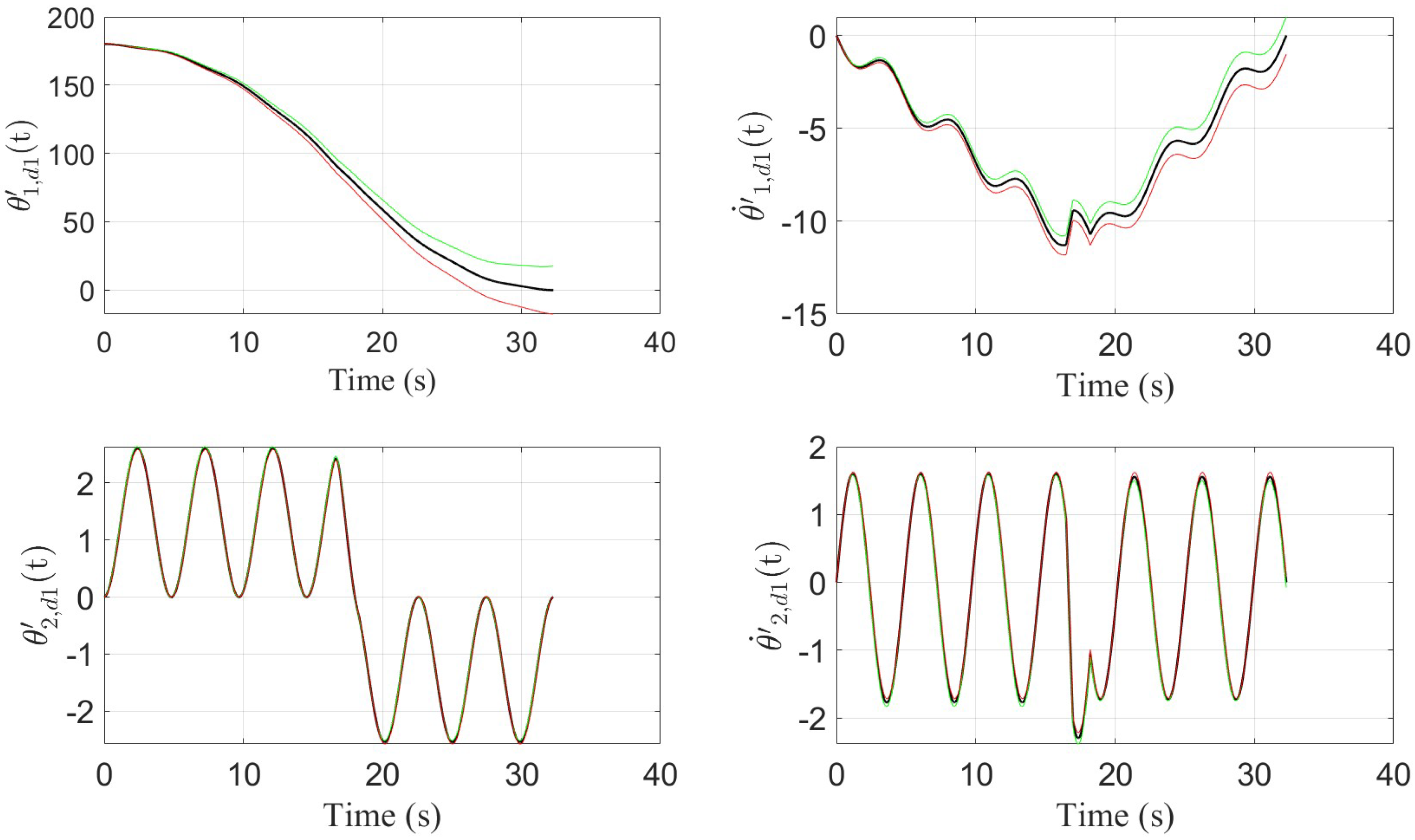
θ 2 , 0 , ( d 1 ) and θ ˙ 2 , 0 , ( d 1 ) , these two terms do not depend on the variances in E 11 and E 22 . Furthermore, f 33 = f 44 . In addition, f 33 , f 34 and f 43 , f 44 are related to the sin and cosine terms, which explains the cyclical/periodic pattern seen in Figure 2 and Figure 3 for θ 2 , 0 , ( d 1 ) and θ ˙ 2 , 0 , ( d 1 ) . For the variance of θ 2 , 0 , ( d 1 ) , the contributions of Var( f 33 E 33 ) and Var( f 34 E 44 ) depend on both σ 3 and σ 4 , the same for θ ˙ 2 , 0 , ( d 1 ) .
Note that notations θ 1 , 0 , ( d 1 ) , θ ˙ 1 , 0 , ( d 1 ) , θ 2 , 0 , ( d 1 ) , and θ ˙ 2 , 0 , ( d 1 ) represent distributions, while θ 1 , 0 , ( d 1 ) (part of the distribution θ 1 , 0 , ( d 1 ) ), θ ˙ 1 , 0 , ( d 1 ) (part of the distribution θ ˙ 1 , 0 , ( d 1 ) ), θ 2 , 0 , ( d 1 ) (part of the distribution θ 2 , 0 , ( d 1 ) ) and θ ˙ 2 , 0 , ( d 1 ) (part of the distribution θ ˙ 2 , 0 , ( d 1 ) ) represent noisy/uncertain states.

5. Examples

Consider a demonstration-scale planar spacecraft (see the schematic diagram in Appendix D) with a 0.27 m (length), 13 kg (mass) base, and a 1 m (length) by 0.02 m (thickness), 0.5 kg (mass) appendage. Additionally, the spring that connects the spacecraft bus to the solar panel has a torsional spring constant of 0.11 N.m/radian. Such parameter values give c 1 = 0.8243 Hz2, c 3 2 = 1.6684 Hz2, b 2 = 6.2419 rad kg−1 m−2 and b 4 = −7.4937 rad kg−1 m−2. Further, | u v | = 0.005 N.m.

5.1. Minimum-Time Control Example

Assume that e 11 = 0.003 rad, e 22 = 0.001 rad/s, e 33 = 0.0015 rad and e 44 = 0.0005 rad/s, although these values are very small, the impact of adding process noise (non-symmetric torque profile) can be clearly seen in the figure (see Figure 2) produced after following the optimization plan presented in Problem (15).
Table 1 shows the values of the position and velocity elements (units are degree and degree/s), and the duration of different switching intervals (unit is second) are also displayed. This table shows the accuracy of the analyses (e.g., θ 2 , 2 , ( d 1 ) θ 2 , 1 , ( d 1 ) + θ 2 , 3 , ( d 1 ) ) performed, as well as the accuracy of the position and velocity values calculated analytically for the flexible mode in Section 3.

5.2. Considering the Process Noise Variance for Minimum-Time Control

The previous section (Section 5) considered the mean of the process noise, and this section considers the variance (or equivalently the standard deviation). Assume that σ 1 = 0.0002 rad, σ 2 = 0.0001 rad/s, σ 3 = 0.0002 rad and σ 4 = 0.0001 rad/s.
Next, assume w = ± 3.5 and w = 0 , the impact of process noise using minimum-time control is shown using Figure 3.
In Figure 3, for all four subplots, w = 0 is plotted using black lines, w = +3.5 is plotted using green lines, and finally, w = −3.5 is plotted using red lines. Figure 2 and Figure 3 are exactly similar when w = 0. Furthermore, the plots for w = ±3.5 are plotted using the minimum-time control torque (the case where w = 0). Of course, all states for w = 0 come to rest (≈0) at t f , ( d 1 ) .
In addition to Figure 3, the trajectory phase-plane plots (for w = ±3.5 and 0) are shown in Figure 4. In Figure 4, the first subplot (left) is the phase-plane plot of the rigid body. The plot is clearly not symmetric, and the influence of three different “w” values is visible. The second subplot (right) is linked to the phase-plane plot of the flexible mode, and this plot is also not symmetric.
In addition, results are summarized for various “w” values at t f , ( d 1 ) using Table 2. Last but not least, in Table 2, all units are degree (position) or degree/s (velocity).

6. Variance-Based Sensitivity Analysis

In this section, the impact of each of the variances on the overall variance in the four angular elements at t f , ( d 1 ) is discussed. The calculation method used in this section is identical to the variance-based sensitivity analysis using first-order Sobol’ indices. Previously, Section 4 analytically discussed the impact of variances. Furthermore, Equation (24) expressed the linear relationship. In addition, to calculate the contribution of each variance, the following calculations (see Equations (25)–(28)) are used.
Ω 11 = Var ( f 11 E 11 ) Var ( θ 1 , 0 , ( d 1 ) ) , Ω 12 = Var ( f 12 E 22 ) Var ( θ 1 , 0 , ( d 1 ) ) , Ω 13 = Var ( f 13 E 33 ) Var ( θ 1 , 0 , ( d 1 ) ) , Ω 14 = Var ( f 14 E 44 ) Var ( θ 1 , 0 , ( d 1 ) )
Ω 21 = Var ( f 21 E 11 ) Var ( θ ˙ 1 , 0 , ( d 1 ) ) , Ω 22 = Var ( f 22 E 22 ) Var ( θ ˙ 1 , 0 , ( d 1 ) ) , Ω 23 = Var ( f 23 E 33 ) Var ( θ ˙ 1 , 0 , ( d 1 ) ) , Ω 24 = Var ( f 24 E 44 ) Var ( θ ˙ 1 , 0 , ( d 1 ) )
Ω 31 = Var ( f 31 E 11 ) Var ( θ 2 , 0 , ( d 1 ) ) , Ω 32 = Var ( f 32 E 22 ) Var ( θ 2 , 0 , ( d 1 ) ) , Ω 33 = Var ( f 33 E 33 ) Var ( θ 2 , 0 , ( d 1 ) ) , Ω 34 = Var ( f 34 E 44 ) Var ( θ 2 , 0 , ( d 1 ) )
Ω 41 = Var ( f 41 E 11 ) Var ( θ ˙ 2 , 0 , ( d 1 ) ) , Ω 42 = Var ( f 42 E 22 ) Var ( θ ˙ 2 , 0 , ( d 1 ) ) , Ω 43 = Var ( f 43 E 33 ) Var ( θ ˙ 2 , 0 , ( d 1 ) ) , Ω 44 = Var ( f 44 E 44 ) Var ( θ ˙ 2 , 0 , ( d 1 ) )
Since f i j is a constant, then Var( f i j E kk ) = f i j 2 Σ k , where i = 1 , 2 , 3 , 4 , j = 1 , 2 , 3 , 4 and k = 1 , 2 , 3 , 4 . Furthermore, the variance in E kk is σ k 2 (defined previously) or Σ k . Finally, Equations (25)–(28) can be expressed analytically as shown in Appendix F (see Equations (A39)–(A54)).
In Equations (A39)–(A54), ϕ 4 = t f , ( d 1 ) = t 43 , ( d 1 ) + t 32 , ( d 1 ) + t 21 , ( d 1 ) + t 10 , ( d 1 ) . Next, the example mentioned in Section 5 is analyzed in more detail. Using the four time intervals ( t 43 , ( d 1 ) , t 32 , ( d 1 ) , t 21 , ( d 1 ) and t 10 , ( d 1 ) ) mentioned in Table 1, the Equations (20)–(23) can be rewritten as follows.
θ 1 , 0 , ( d 1 ) = 32.29056 e 11 + 521.34043 e 22 + 16.24552 e 33 + 257.08912 e 44 0.77112
θ ˙ 1 , 0 , ( d 1 ) = 32.29057 e 22 + 0.81344 e 33 + 16.24552 e 44 0.041633
θ 2 , 0 , ( d 1 ) = 0.59069 e 33 + 0.98682 e 44 + 0.00039
θ ˙ 2 , 0 , ( d 1 ) = 1.64642 e 33 0.59069 e 44 + 0.00276
Equations (29)–(32) show the correctness of Equations (A19) to (A38). In summary, Equations (29)–(32) also show numerically that f 11 = f 22 and f 33 = f 44 . Additionally, f 12 = 1 2 ( f 11 ) 2 . Furthermore, consider a situation where σ 1 and σ 2 are 0, then the position and velocity of the spacecraft bus will also have some uncertainty due to the variances of E 33 and E 44 .
Using Equations (A39)–(A54), the impact of each variance term is summarized in Table 3. Note that since f 21 = f 31 = f 32 = f 41 = f 42 = 0, therefore, the values of Ω 21 , Ω 31 , Ω 32 , Ω 41 and Ω 42 are all 0.
Using Table 3, it can be stated that for the mentioned configuration, for θ 1 , 0 , ( d 1 ) , 79% of the variance is caused by Ω 12 . In addition, Ω 11 and Ω 13 both have negligible impact. For θ ˙ 1 , 0 , ( d 1 ) , the majority of the variance is caused by Ω 22 , while Ω 23 has a very small or negligible impact. For θ 2 , 0 , ( d 1 ) , Ω 33 and Ω 34 contributed almost equally. Finally, for θ ˙ 2 , 0 , ( d 1 ) , Ω 43 is responsible for about 97% of the total variance.
As mentioned earlier, to compute Sobol’ indices, python library “scipy.stats.sobol_indices” (https:/docs.scipy.org/doc/scipy-1.14.1/reference/generated/scipy.stats.sobol_indices.html, (accessed on 19 October 2024)) is used and the results are presented in Appendix A using Table A1, which is identical to the result mentioned in Table 3.

7. Conclusions

This article analyzed various impacts of process noise for minimum-time rest-to-rest control for a spacecraft bus attached to a flexible mode by a torsional spring. The first part of the article analytically presented the flexible mode switching equations and derived key equations related to rigid and flexible modes at the mid/central switch. In addition, the use of the MultiStart algorithm makes it possible to solve the minimum-time rest-to-rest control problem in the presence of the process noise. The second part of the article deals more with process noise variance; using a list of equations, the impacts of the variances are analyzed. The analytic variance-based sensitivity analysis procedure discussed in this article produces results identical to those produced by the Sobol’ indices.

Funding

The project or effort undertaken was or is sponsored by the Department of the Navy, Office of Naval Research, Consortium for Robotics Unmanned Systems Education and Research at the Naval Postgraduate School.

Data Availability Statement

No new data were created or analyzed in this study.

Acknowledgments

Shambo Bhattacharjee would like to thank his postdoctoral advisor, Jennifer Hudson (Mechanical and Aerospace Engineering, Naval Postgraduate School) for her unconditional help, support, and valuable comments.

Conflicts of Interest

The authors declare no conflicts of interest.

Nomenclature

  • The following nomenclature are used in this manuscript:
θ 1 Rigid body position (ideal dynamics)
θ ˙ 1 Rigid body velocity (ideal dynamics)
θ 2 Flexible mode position (ideal dynamics)
θ ˙ 1 Flexible mode velocity (ideal dynamics)
c 1 Coupling parameter (constant)
c 3 Flexible mode natural frequency (constant)
U = | u v |                                  Torque magnitude (constant)
u m i n Minimum torque magnitude limit (constant)
u m a x Maximum torque magnitude limit (constant)
tTime
θ 0 Slewing angle (constant)
b 2 Input parameter (constant)
b 4 Input parameter (constant)
ϵ = [ e 11 , e 22 , e 33 , e 44 ] T Process noise mean
iNumber of flexible modes
t f Total time or the final time (ideal dynamics)
t f , ( d 1 ) Total time or the final time (uncertain dynamics)
[ t 43 , t 32 , t 21 , t 10 ] T Switching time intervals (ideal dynamics)
[ t 43 , ( d 1 ) , t 32 , ( d 1 ) , t 21 , ( d 1 ) , t 10 , ( d 1 ) ] T Switching time intervals (uncertain dynamics)
wWeighting factor
t ( v ) ( v 1 ) , ( d 1 ) Switching time interval representation (uncertain dynamics)
t ( v ) ( v 1 ) Switching time interval representation (ideal dynamics)
[ θ 2 , 3 , ( d 1 ) , θ 2 , 2 , ( d 1 ) , θ 2 , 1 , ( d 1 ) ] T Flexible mode positions at V3, V2 and V1, respectively, (uncertain dynamics)
[ θ ˙ 2 , 3 , ( d 1 ) , θ ˙ 2 , 2 , ( d 1 ) , θ ˙ 2 , 1 , ( d 1 ) ] T Flexible mode velocities at V3, V2 and V1, respectively, (uncertain dynamics)
[ θ 1 , 3 , ( d 1 ) , θ 1 , 2 , ( d 1 ) , θ 1 , 1 , ( d 1 ) ] T Rigid body positions at V3, V2 and V1, respectively, (uncertain dynamics)
[ θ ˙ 1 , 3 , ( d 1 ) , θ ˙ 1 , 2 , ( d 1 ) , θ ˙ 1 , 1 , ( d 1 ) ] T Rigid body velocities at V3, V2 and V1, respectively, (uncertain dynamics)
σ = diag [ σ 1 , σ 2 , σ 3 , σ 4 ] Process noise standard deviation
Σ = diag [ Σ 1 , Σ 2 , Σ 3 , Σ 4 ] Process noise variance
[ δ 1 , δ 2 , δ 3 ] T Represent the differences between process noise affected and unaffected time intervals
t 0 Initial time

Appendix A. Sobol’s First-Order Variance-Based Sensitivity Analysis Results

Sobol’s first-order variance-based sensitivity analysis results are presented below (see Table A1).
Table A1. Analysis of variance-based sensitivity using first order Sobol’ indices. Note that i = 1 , 2 , 3 , 4 .
θ 0 , ( d 1 ) S i 1 S i 2 S i 3 S i 4
θ 1 , 0 , ( d 1 ) 0.012370.790160.003560.19250
θ ˙ 1 , 0 , ( d 1 ) 00.793300.001820.20215
θ 2 , 0 . ( d 1 ) 000.588230.40943
θ ˙ 2 , 0 . ( d 1 ) 000.969140.03140
The results mentioned in Table A1 are identical to the result obtained using Table 3. In addition, the results mentioned in Table A1 are also plotted (see Figure A1a,b and Figure A2a,b) and are shown below.
Figure A1. Variance-based sensitivity analysis for rigid body trajectory. (a) Variance-based sensitivity analysis for θ 1 , 0 , ( d 1 ) . (b) Variance-based sensitivity analysis for θ ˙ 1 , 0 , ( d 1 ) .
Mathematics 13 01144 g0a1
Figure A2. Variance-based sensitivity analysis for flexible mode trajectory. (a) Variance-based sensitivity analysis for θ 2 , 0 , ( d 1 ) . (b) Variance-based sensitivity analysis for θ ˙ 2 , 0 , ( d 1 ) .
Mathematics 13 01144 g0a2
Figure A1a,b and Figure A2a,b visually illustrate the results mentioned in Table A1 for the four angular elements at t f , ( d 1 ) . In the Figure A1a, the horizontal axis represents S 11 , S 12 , S 13 , and S 14 (the first row of Table A1). Figure A1b represents the three elements contributing to variance related to ( θ ˙ 1 , 0 , ( d 1 ) ), note that S 21 is not displayed as this does not contribute to the overall variance. Likewise, in Figure A2a,b, only the impacts of S 33 , S 34 and S 43 , S 44 (i.e., non-zero elements) are displayed.

Appendix B. Phase-Plane Equations

(1)
Rigid body phase-plane equation.
Using Equation (10) (formula for computing t ( v ) ( v 1 ) , ( d 1 ) ) in Equation (6), the phase-plane equation of the rigid body (coupled with the flexible mode equation) can be written as follows.
( c 3 2 θ 1 , v 1 , ( d 1 ) + c 1 θ 2 , v 1 , ( d 1 ) ) ( c 3 2 θ 1 , v , ( d 1 ) + c 1 θ 2 , v , ( d 1 ) ) = ( c 3 2 θ ˙ 1 , v 1 , ( d 1 ) + c 1 θ ˙ 2 , v 1 , ( d 1 ) ) 2 ( c 3 2 θ ˙ 1 , v , ( d 1 ) + c 1 θ ˙ 2 , v , ( d 1 ) ) 2 2 ( b 2 c 3 2 u v + b 4 c 1 u v + c 1 e 44 + c 3 2 e 22 ) + ( c 3 2 θ ˙ 1 , v 1 , ( d 1 ) + c 1 θ ˙ 2 , v 1 , ( d 1 ) ) ( c 3 2 θ ˙ 1 , v , ( d 1 ) + c 1 θ ˙ 2 , v , ( d 1 ) ) ( b 2 c 3 2 u v + b 4 c 1 u v + c 1 e 44 + c 3 2 e 22 ) ( c 3 2 e 11 + c 1 e 33 )
(2)
Flexible mode phase-plane equation.
Using Equations (8)–(10), the flexible mode phase-plane equation can be obtained and is written as follows.
( c 3 θ 2 , v 1 , ( d 1 ) e 44 c 3 b 4 u v c 3 ) 2 + ( θ ˙ 2 , v 1 , ( d 1 ) + e 33 ) 2 = ( c 3 θ 2 , v , ( d 1 ) e 44 c 3 b 4 u v c 3 ) 2 + ( θ ˙ 2 , v , ( d 1 ) + e 33 ) 2
Using the flexible mode phase-plane equation, the following two relationships can be obtained.
-
θ ˙ 2 , 2 , ( d 1 ) takes the following form.
( θ ˙ 2 , 2 , ( d 1 ) + e 33 ) 2 = ( e 44 c 3 + b 4 u 1 c 3 ) 2 + ( e 33 ) 2 ( c 3 θ 2 , 1 , ( d 1 ) e 44 c 3 b 4 u 1 c 3 ) 2 ( c 3 θ 2 , 2 , ( d 1 ) e 44 c 3 b 4 u 2 c 3 ) 2 + ( c 3 θ 2 , 1 , ( d 1 ) e 44 c 3 b 4 u 2 c 3 ) 2
Additionally, θ ˙ 2 , 2 , ( d 1 ) can also be written as follows.
( θ ˙ 2 , 2 , ( d 1 ) + e 33 ) 2 = ( e 44 c 3 + b 4 u 4 c 3 ) 2 + ( e 33 ) 2 ( c 3 θ 2 , 3 , ( d 1 ) e 44 c 3 b 4 u 4 c 3 ) 2 ( c 3 θ 2 , 2 , ( d 1 ) e 44 c 3 b 4 u 3 c 3 ) 2 + ( c 3 θ 2 , 3 , ( d 1 ) e 44 c 3 b 4 u 3 c 3 ) 2
(3)
Representing the switching interval time values.
t 43 , ( d 1 ) = ( c 3 2 θ ˙ 1 , 3 , ( d 1 ) + c 1 θ ˙ 2 , 3 , ( d 1 ) ) ( b 4 c 1 u 4 + b 2 c 3 2 u 4 + c 1 e 44 + c 3 2 e 22 )
t 32 , ( d 1 ) = ( c 3 2 θ ˙ 1 , 2 , ( d 1 ) + c 1 θ ˙ 2 , 2 , ( d 1 ) ) ( c 3 2 θ ˙ 1 , 3 , ( d 1 ) + c 1 θ ˙ 2 , 3 , ( d 1 ) ) ( b 4 c 1 u 3 + b 2 c 3 2 u 3 + c 1 e 44 + c 3 2 e 22 )
t 21 , ( d 1 ) = ( c 3 2 θ ˙ 1 , 1 , ( d 1 ) + c 1 θ ˙ 2 , 1 , ( d 1 ) ) ( c 3 2 θ ˙ 1 , 2 , ( d 1 ) + c 1 θ ˙ 2 , 2 , ( d 1 ) ) ( b 4 c 1 u 2 + b 2 c 3 2 u 2 + c 1 e 44 + c 3 2 e 22 )
t 10 , ( d 1 ) = ( c 3 2 θ ˙ 1 , 1 , ( d 1 ) + c 1 θ ˙ 2 , 1 , ( d 1 ) ) ( b 4 c 1 u 1 + b 2 c 3 2 u 1 + c 1 e 44 + c 3 2 e 22 )
(4)
Δ θ e , ( d 1 ) takes the following form.
Δ θ e , ( d 1 ) = ( c 3 2 θ ˙ 1 , 2 , ( d 1 ) + c 1 θ ˙ 2 , 2 , ( d 1 ) ) 2 ( c 3 2 θ ˙ 1 , 3 , ( d 1 ) + c 1 θ ˙ 2 , 3 , ( d 1 ) ) 2 + ( c 3 2 θ ˙ 1 , 1 , ( d 1 ) + c 1 θ ˙ 2 , 1 , ( d 1 ) ) 2 2 ( b 2 c 3 2 u 3 + b 4 c 1 u 3 + c 1 e 44 + c 3 2 e 22 ) + ( c 3 2 θ ˙ 1 , 3 , ( d 1 ) + c 1 θ ˙ 2 , 3 , ( d 1 ) ) 2 ( c 3 2 θ ˙ 1 , 1 , ( d 1 ) + c 1 θ ˙ 2 , 1 , ( d 1 ) ) 2 + ( c 3 2 θ ˙ 1 , 2 , ( d 1 ) + c 1 θ ˙ 2 , 2 , ( d 1 ) ) 2 2 ( b 2 c 3 2 u 4 + b 4 c 1 u 4 + c 1 e 44 + c 3 2 e 22 ) + [ c 3 2 e 11 + c 1 e 33 ] [ ( c 3 2 θ ˙ 1 , 2 , ( d 1 ) + c 1 θ ˙ 2 , 2 , ( d 1 ) ) ( c 3 2 θ ˙ 1 , 3 , ( d 1 ) + c 1 θ ˙ 2 , 3 , ( d 1 ) ) + ( c 3 2 θ ˙ 1 , 1 , ( d 1 ) + c 1 θ ˙ 2 , 1 , ( d 1 ) ) ] 2 ( b 2 c 3 2 u 3 + b 4 c 1 u 3 + c 1 e 44 + c 3 2 e 22 ) + [ c 3 2 e 11 + c 1 e 33 ] [ ( c 3 2 θ ˙ 1 , 3 , ( d 1 ) + c 1 θ ˙ 2 , 3 , ( d 1 ) ) ( c 3 2 θ ˙ 1 , 1 , ( d 1 ) + c 1 θ ˙ 2 , 1 , ( d 1 ) ) + ( c 3 2 θ ˙ 1 , 2 , ( d 1 ) + c 1 θ ˙ 2 , 2 , ( d 1 ) ) ] 2 ( b 2 c 3 2 u 4 + b 4 c 1 u 4 + c 1 e 44 + c 3 2 e 22 )

Appendix C. Linking Process Noise Affected and Unaffected Dynamics

Equation (11) can be written as follows.
θ ˙ 2 , 3 , ( d 1 ) = ( e 44 sin ( c 3 α 1 ( 1 + x 1 ) ) c 3 e 33 + c 3 e 33 cos ( c 3 α 1 ( 1 + x 1 ) ) + b 4 u 4 sin ( c 3 α 1 ( 1 + x 1 ) ) ) / c 3
θ ˙ 2 , 2 , ( d 1 ) = ( e 44 sin ( c 3 α 2 ( 1 + x 2 ) ) c 3 e 33 + c 3 e 33 cos ( c 3 α 2 ( 1 + x 2 ) ) + b 4 u 4 sin ( c 3 α 2 ( 1 + x 2 ) ) 2 b 4 u 4 sin ( c 3 ( α 2 α 1 ) ( 1 + x 21 ) ) ) / c 3
θ ˙ 2 , 1 , ( d 1 ) = ( e 44 sin ( c 3 α 3 ( 1 + x 3 ) ) c 3 e 33 + c 3 e 33 cos ( c 3 α 3 ( 1 + x 3 ) ) + b 4 u 4 sin ( c 3 α 3 ( 1 + x 3 ) ) 2 b 4 u 4 sin ( c 3 ( α 3 α 1 ) ( 1 + x 31 ) ) + 2 b 4 u 4 sin ( c 3 ( α 3 α 2 ) ( 1 + x 32 ) ) ) / c 3
Similarly, Equation (12) can be written in the following form.
θ 2 , 3 , ( d 1 ) = ( e 44 + b 4 u 4 e 44 cos ( c 3 α 1 ( 1 + x 1 ) ) b 4 u 4 cos ( c 3 α 1 ( 1 + x 1 ) ) + c 3 e 33 sin ( c 3 α 1 ( 1 + x 1 ) ) ) / c 3 2
θ 2 , 2 , ( d 1 ) = ( e 44 e 44 cos ( c 3 α 2 ( 1 + x 2 ) ) b 4 u 4 b 4 u 4 cos ( c 3 α 2 ( 1 + x 2 ) ) + c 3 e 33 sin ( c 3 ( α 2 ) ( 1 + x 2 ) ) + 2 b 4 u 4 cos ( c 3 ( α 2 α 1 ) ( 1 + x 21 ) ) ) / c 3 2
θ 2 , 1 , ( d 1 ) = ( e 44 + b 4 u 4 e 44 cos ( c 3 α 3 ( 1 + x 3 ) ) b 4 u 4 cos ( c 3 α 3 ( 1 + x 3 ) ) + c 3 e 33 sin ( c 3 α 3 ( 1 + x 3 ) ) + 2 b 4 u 4 cos ( c 3 ( α 3 α 1 ) ( 1 + x 31 ) ) 2 b 4 u 4 cos ( c 3 ( α 3 α 2 ) ( 1 + x 32 ) ) ) / c 3 2
In Equations (A10)–(A15), α and x related terms are defined below.
α 1 = t 43 , α 2 = t 43 + t 32 , α 3 = t 43 + t 32 + t 21
ϕ 1 = α 1 + δ 1 , ϕ 2 = α 2 + δ 2 , ϕ 3 = α 3 + δ 3
x 1 = δ 1 α 1 , x 2 = δ 2 α 2 , x 3 = δ 3 α 3 , x 21 = δ 2 δ 1 α 2 α 1 , x 31 = δ 3 δ 1 α 3 α 1 , x 32 = δ 3 δ 2 α 3 α 2
Equations (11) and (12) include the ϕ terms that are related to the process noise-affected time values, whereas the α terms are associated with the ideal/exact or process noise “unaffected” time values (see Equation (A16)). In addition, Equation (A17) showed the relation between ϕ and α . The δ terms indicate small deviations; another way to interpret the δ terms in Equation (A17) is that they represent the difference between the process noise-affected minimum-time control and the process noise “unaffected” minimum-time control at various time steps. If the angular values at three switching points related to the flexible mode of an ideal system (process noise unaffected) are represented by the notations θ 2 , 3 , θ 2 , 2 , θ 2 , 1 (representing positions) and θ ˙ 2 , 3 , θ ˙ 2 , 2 , θ ˙ 2 , 1 (representing velocities) at V 3 , V 2 , and V 1 , then θ v , v 1 , ( d 1 ) = θ v , v 1 (or θ v , v 1 , ( d 1 ) θ v , v 1 ), if the following equations are true.
(a)
e 11 = e 22 = e 33 = e 44 = 0 (or ≈ 0) and
(b)
x 1 = x 2 = x 3 = x 21 = x 31 = x 32 = 0 (or ≈ 0) or δ 1 = δ 2 = δ 3 = 0 (or ≈ 0)
where θ 2 , ( d 1 ) is related to the position and velocity of the uncertain dynamics (related to the flexible mode), while θ 2 is related to the position and velocity of the ideal dynamics.

Appendix D. A Brief Description of the Model Used
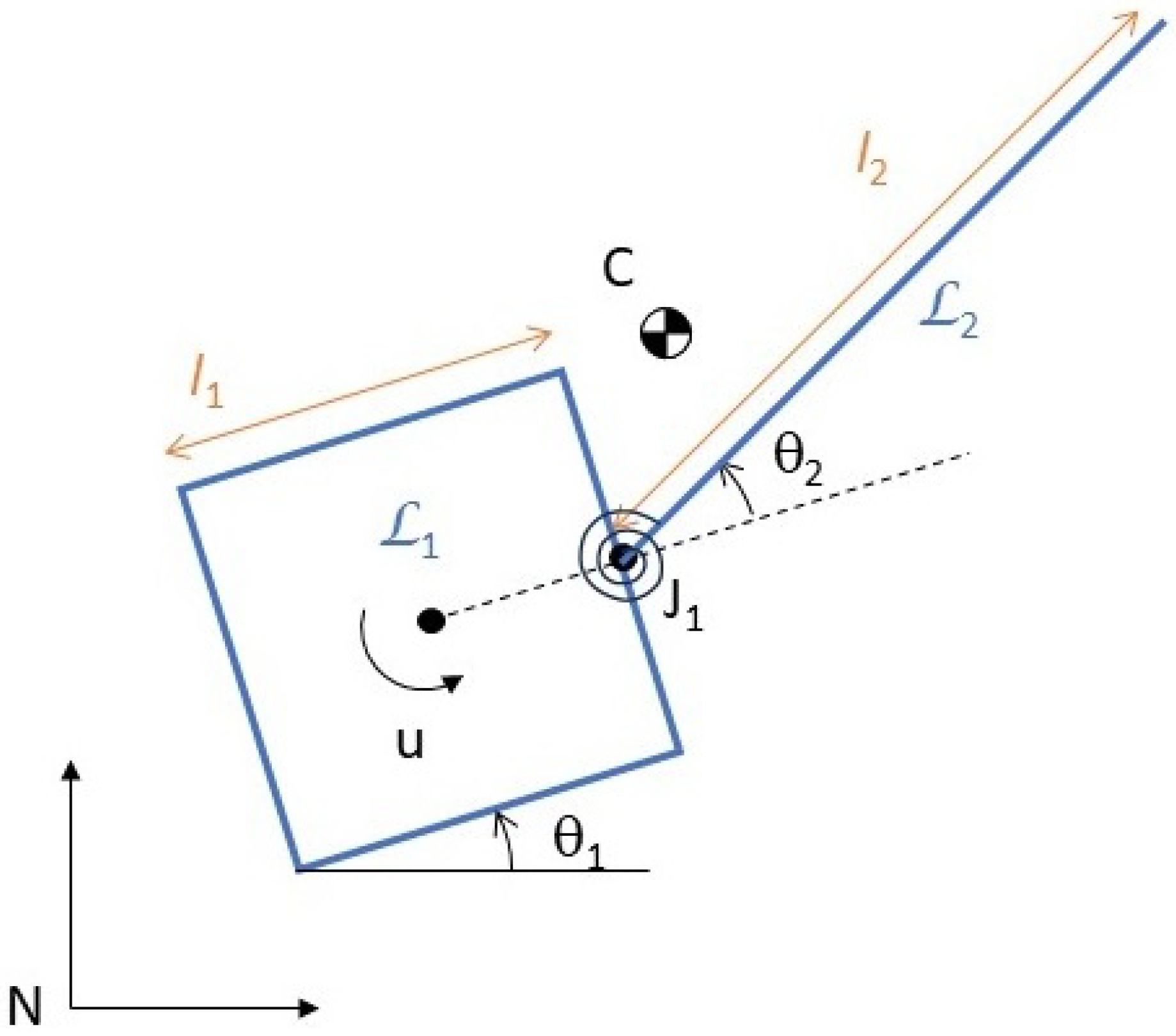
This article studies a simple two-body mass-spring system. The first body ( L 1 ) represents a cubic-shaped spacecraft bus. The second body, ( L 2 ), is a thin plate (solar panel). Furthermore, the first and second bodies are connected by a torsion spring. Figure A3 illustrates the schematic diagram, where L 1 and L 2 appear as a square plate of length l 1 and a rectangular plate of length l 2 , respectively. The articulation point of ( L 1 ) and ( L 2 ) is indicated by J1. The torsion spring connecting ( L 1 ) and ( L 2 ) has a spring constant k. The point C indicates the center of mass and u indicates the torque. Moreover, the two bodies are homogeneous.
Figure A3. Schematic of a free-floating two-rigid-body, torsional-spring-joint system, in flat space.
Mathematics 13 01144 g0a3
As mentioned earlier, this article considers a planar motion. Last but not least θ 1 is the absolute orientation of the first body, while θ 2 is the relative orientation of the second body with respect to the first body.
The linearized equation of motion of this system is represented by Equation (1), where each term is described in more detail by Equation (2). However, the main interest of this article is to understand the impact of process noise. The uncertain state equation is, therefore, derived (Equation (3)) and further analyses are performed.

Appendix E. Further Analysis of the Matrix Terms

The terms mentioned in the Matrix (24) are analyzed in more detail below.
f 11 = t 43 , ( d 1 ) + t 32 , ( d 1 ) + t 21 , ( d 1 ) + t 10 , ( d 1 )
f 12 = 1 2 ( t 43 , ( d 1 ) + t 32 , ( d 1 ) + t 21 , ( d 1 ) + t 10 , ( d 1 ) ) 2
f 13 = c 1 ( sin ( c 3 t 43 , ( d 1 ) + c 3 t 32 , ( d 1 ) + c 3 t 21 , ( d 1 ) + c 3 t 10 , ( d 1 ) ) ) / c 3 3 + c 1 ( t 43 , ( d 1 ) + t 32 , ( d 1 ) + t 21 , ( d 1 ) + t 10 , ( d 1 ) ) / c 3 2
f 14 = c 1 ( 1 + cos ( c 3 ( t 43 , ( d 1 ) + t 32 , ( d 1 ) + t 21 , ( d 1 ) + t 10 , ( d 1 ) ) ) ) / c 3 4 + 1 2 c 1 ( t 43 , ( d 1 ) + t 32 , ( d 1 ) + t 21 , ( d 1 ) + t 10 , ( d 1 ) ) 2 / c 3 2
Υ 1 = θ 0 + b 2 u 4 ( t 43 , ( d 1 ) 2 t 32 , ( d 1 ) 2 t 10 , ( d 1 ) 2 + t 21 , ( d 1 ) 2 ) / 2 + b 2 t 32 , ( d 1 ) u 4 ( t 43 , ( d 1 ) t 10 , ( d 1 ) ) + b 2 u 4 ( t 43 , ( d 1 ) t 10 , ( d 1 ) t 32 , ( d 1 ) t 21 , ( d 1 ) + t 43 , ( d 1 ) t 21 , ( d 1 ) + t 10 , ( d 1 ) t 21 , ( d 1 ) ) + b 4 c 1 u 4 ( t 43 , ( d 1 ) 2 t 10 , ( d 1 ) 2 + t 21 , ( d 1 ) 2 t 32 , ( d 1 ) 2 ) / ( 2 c 3 2 ) + b 4 c 1 u 4 ( cos ( c 3 ( t 43 , ( d 1 ) + t 32 , ( d 1 ) + t 21 , ( d 1 ) + t 10 , ( d 1 ) ) ) + 2 cos ( c 3 ( t 21 , ( d 1 ) + t 10 , ( d 1 ) ) ) 2 cos ( c 3 ( t 32 , ( d 1 ) + t 21 , ( d 1 ) + t 10 , ( d 1 ) ) ) + 1 2 cos ( c 3 t 10 , ( d 1 ) ) ) / c 3 4 + b 4 c 1 u 4 ( t 10 , ( d 1 ) t 21 , ( d 1 ) t 32 , ( d 1 ) t 21 , ( d 1 ) + t 43 , ( d 1 ) t 10 , ( d 1 ) + t 43 , ( d 1 ) t 21 , ( d 1 ) + t 32 , ( d 1 ) t 43 , ( d 1 ) t 32 , ( d 1 ) t 10 , ( d 1 ) ) / c 3 2
f 21 = 0
f 22 = t 43 , ( d 1 ) + t 32 , ( d 1 ) + t 21 , ( d 1 ) + t 10 , ( d 1 )
f 23 = c 1 ( 1 cos ( c 3 ( t 43 , ( d 1 ) + t 32 , ( d 1 ) + t 21 , ( d 1 ) + t 10 , ( d 1 ) ) ) ) / c 3 2
f 24 = c 1 ( c 3 ( t 43 , ( d 1 ) + t 32 , ( d 1 ) + t 21 , ( d 1 ) + t 10 , ( d 1 ) ) sin ( c 3 ( t 43 , ( d 1 ) + t 32 , ( d 1 ) + t 21 , ( d 1 ) + t 10 , ( d 1 ) ) ) ) / c 3 3
Υ 2 = b 4 c 1 u 4 ( 2 sin ( c 3 ( t 32 , ( d 1 ) + t 21 , ( d 1 ) + t 10 , ( d 1 ) ) ) sin ( c 3 ( t 43 , ( d 1 ) + t 32 , ( d 1 ) + t 21 , ( d 1 ) + t 10 , ( d 1 ) ) ) 2 sin ( c 3 ( t 21 , ( d 1 ) + t 10 , ( d 1 ) ) ) + 2 sin ( c 3 t 10 , ( d 1 ) ) ) / c 3 3 + b 2 ( t 43 , ( d 1 ) t 32 , ( d 1 ) t 10 , ( d 1 ) + t 21 , ( d 1 ) ) + b 4 c 1 ( t 43 , ( d 1 ) t 32 , ( d 1 ) + t 21 , ( d 1 ) t 10 , ( d 1 ) ) / c 3 2
f 31 = 0
f 32 = 0
f 33 = sin ( c 3 ( t 43 , ( d 1 ) + t 32 , ( d 1 ) + t 21 , ( d 1 ) + t 10 , ( d 1 ) ) ) / c 3
f 34 = ( 1 cos ( c 3 ( t 43 , ( d 1 ) + t 32 , ( d 1 ) + t 21 , ( d 1 ) + t 10 , ( d 1 ) ) ) ) / c 3 2
Υ 3 = b 4 u 4 ( cos ( c 3 ( t 43 , ( d 1 ) + t 32 , ( d 1 ) + t 21 , ( d 1 ) + t 10 , ( d 1 ) ) ) + 2 cos ( c 3 ( t 21 , ( d 1 ) + t 10 , ( d 1 ) ) ) 2 cos ( c 3 t 10 , ( d 1 ) ) 2 cos ( c 3 ( t 32 , ( d 1 ) + t 21 , ( d 1 ) + t 10 , ( d 1 ) ) ) + 1 ) / c 3 2
f 41 = 0
f 42 = 0
f 43 = cos ( c 3 ( t 43 , ( d 1 ) + t 32 , ( d 1 ) + t 21 , ( d 1 ) + t 10 , ( d 1 ) ) ) 1
f 44 = sin ( c 3 ( t 43 , ( d 1 ) + t 32 , ( d 1 ) + t 21 , ( d 1 ) + t 10 , ( d 1 ) ) ) / c 3
Υ 4 = b 4 u 4 ( sin ( c 3 ( t 43 , ( d 1 ) + t 32 , ( d 1 ) + t 21 , ( d 1 ) + t 10 , ( d 1 ) ) ) 2 sin ( c 3 ( t 32 , ( d 1 ) + t 21 , ( d 1 ) + t 10 , ( d 1 ) ) ) + 2 sin ( c 3 ( t 21 , ( d 1 ) + t 10 , ( d 1 ) ) ) 2 sin ( c 3 t 10 , ( d 1 ) ) ) / c 3

Appendix F. Further Analysis of the Variance-Based Sensitivity Analysis Terms

The sensitivity analysis terms are presented analytically below.
Ω 11 = Σ 1 ϕ 4 2 Σ 1 ϕ 4 2 + 0.25 Σ 2 ϕ 4 4 + ( c 1 2 Σ 3 ( sin ( c 3 ϕ 4 ) c 3 ϕ 4 ) 2 ) / c 3 6 + ( c 1 2 Σ 4 ( 2 cos ( c 3 ϕ 4 ) + c 3 2 ϕ 4 2 2 ) 2 ) / ( 4 c 3 8 )
Ω 12 = 0.25 Σ 2 ϕ 4 4 Σ 1 ϕ 4 2 + 0.25 Σ 2 ϕ 4 4 + ( c 1 2 Σ 3 ( sin ( c 3 ϕ 4 ) c 3 ϕ 4 ) 2 ) / c 3 6 + ( c 1 2 Σ 4 ( 2 cos ( c 3 ϕ 4 ) + c 3 2 ϕ 4 2 2 ) 2 ) / ( 4 c 3 8 )
Ω 13 = c 1 2 Σ 3 ( sin ( c 3 ϕ 4 ) c 3 ϕ 4 ) 2 c 3 6 ( Σ 1 ϕ 4 2 + 0.25 Σ 2 ϕ 4 4 + ( c 1 2 Σ 3 ( sin ( c 3 ϕ 4 ) c 3 ϕ 4 ) 2 ) / c 3 6 + ( c 1 2 Σ 4 ( 2 cos ( c 3 ϕ 4 ) + c 3 2 ϕ 4 2 2 ) 2 ) / ( 4 c 3 8 ) )
Ω 14 = c 1 2 Σ 4 ( 2 cos ( c 3 ϕ 4 ) + c 3 2 ϕ 4 2 2 ) 2 4 c 3 8 ( Σ 1 ϕ 4 2 + 0.25 Σ 2 ϕ 4 4 + ( c 1 2 Σ 3 ( sin ( c 3 ϕ 4 ) c 3 ϕ 4 ) 2 ) / c 3 6 + ( c 1 2 Σ 4 ( 2 cos ( c 3 ϕ 4 ) + c 3 2 ϕ 4 2 2 ) 2 ) / ( 4 c 3 8 ) )
Ω 21 = 0
Ω 22 = Σ 2 ϕ 4 2 Σ 2 ϕ 4 2 + ( c 1 2 Σ 4 ( sin ( c 3 ϕ 4 ) c 3 ϕ 4 ) 2 ) / c 3 6 + ( c 1 2 Σ 3 ( cos ( c 3 ϕ 4 ) 1 ) 2 ) / c 3 4
Ω 23 = c 1 2 Σ 3 ( cos ( c 3 ϕ 4 ) 1 ) 2 c 3 4 ( Σ 2 ϕ 4 2 + ( c 1 2 Σ 4 ( sin ( c 3 ϕ 4 ) c 3 ϕ 4 ) 2 ) / c 3 6 + ( c 1 2 Σ 3 ( cos ( c 3 ϕ 4 ) 1 ) 2 ) / c 3 4 )
Ω 24 = c 1 2 Σ 4 ( sin ( c 3 ϕ 4 ) c 3 ϕ 4 ) 2 c 3 6 ( Σ 2 ϕ 4 2 + ( c 1 2 Σ 4 ( sin ( c 3 ϕ 4 ) c 3 ϕ 4 ) 2 ) / c 3 6 + ( c 1 2 Σ 3 ( cos ( c 3 ϕ 4 ) 1 ) 2 ) / c 3 4 )
Ω 31 = 0
Ω 32 = 0
Ω 33 = Σ 3 ( sin ( c 3 ϕ 4 ) ) 2 c 3 2 ( ( Σ 4 ( cos ( c 3 ϕ 4 ) 1 ) 2 ) / c 3 4 + Σ 3 ( sin ( c 3 ϕ 4 ) ) 2 / c 3 2 )
Ω 34 = Σ 4 ( cos ( c 3 ϕ 4 ) 1 ) 2 c 3 4 ( ( Σ 4 ( cos ( c 3 ϕ 4 ) 1 ) 2 ) / c 3 4 + Σ 3 ( sin ( c 3 ϕ 4 ) ) 2 / c 3 2 )
Ω 41 = 0
Ω 42 = 0
Ω 43 = Σ 3 ( cos ( c 3 ϕ 4 ) 1 ) 2 Σ 3 ( cos ( c 3 ϕ 4 ) 1 ) 2 + Σ 4 ( sin ( c 3 ϕ 4 ) ) 2 / c 3 2
Ω 44 = Σ 4 ( sin ( c 3 ϕ 4 ) ) 2 c 3 2 ( Σ 3 ( cos ( c 3 ϕ 4 ) 1 ) 2 + Σ 4 ( sin ( c 3 ϕ 4 ) ) 2 / c 3 2 )

References

  1. Yang, H.; Krishnan, H.; Ang, M. A simple rest-to-rest control command for a flexible link robot. In Proceedings of the International Conference on Robotics and Automation, Albuquerque, NM, USA, 20–25 April 1997; Volume 4, pp. 3312–3317. [Google Scholar] [CrossRef]
  2. Kim, J.J.; Agrawal, B.N. Rest-to-rest slew maneuver of three-axis rotational flexible spacecraft. IFAC Proc. Vol. 2008, 41, 12054–12060. [Google Scholar] [CrossRef]
  3. Singh, G.; Kabamba, P.T.; Mcclamroch, N.H. Planar, time-optimal, rest-to-rest slewing maneuvers of flexible spacecraft. J. Guid. Control Dyn. 1989, 12, 71–81. [Google Scholar] [CrossRef]
  4. Barbieri, E.; Ozguner, U. A new minimum-time control law for a one-mode model of a flexible slewing structure. IEEE Trans. Autom. Control 1993, 38, 142–146. [Google Scholar] [CrossRef]
  5. Pao, L.Y. Minimum-time control characteristics of flexible structures. J. Guid. Control Dyn. 1996, 19, 123–129. [Google Scholar] [CrossRef]
  6. Albassam, B.A. Optimal Near-Minimum-Time Control Design for Flexible Structures. J. Guid. Control Dyn. 2002, 25, 618–625. [Google Scholar] [CrossRef]
  7. Hartmann, R.; Singh, T. Fuel/Time Optimal Control of Flexible Space Structures: A Frequency Domain Approach. J. Vib. Control 1999, 5, 795–817. [Google Scholar] [CrossRef]
  8. Pao, L.Y.; Singhose, W.E. Robust minimum time control of flexible structures. Automatica 1998, 34, 229–236. [Google Scholar] [CrossRef]
  9. Naidu, S.A.; Leifsson, L.T. Multidisciplinary Spacecraft and Trajectory Uncertainty Quantification for an Interplanetary Mission. In Proceedings of the AIAA SCITECH 2024 Forum, Orlando, FL, USA, 8–12 January 2024. [Google Scholar] [CrossRef]
  10. Zhang, A.; Wang, Y.; Zhang, Z.; Karimi, H.R.; Sun, W. Robust Control Allocation for Spacecraft Attitude Stabilization under Actuator Faults and Uncertainty. Math. Probl. Eng. 2014, 2014, 789327. [Google Scholar] [CrossRef]
  11. Federici, L.; Zavoli, A. Robust interplanetary trajectory design under multiple uncertainties via meta-reinforcement learning. Acta Astronaut. 2024, 214, 147–158. [Google Scholar] [CrossRef]
  12. Yuan, H.; Li, D.; He, G.; Wang, J. Uncertainty-resilient constrained rendezvous trajectory optimization via stochastic feedback control and unscented transformation. Acta Astronaut. 2024, 219, 264–277. [Google Scholar] [CrossRef]
  13. Cognetti, M.; Salaris, P.; Robuffo Giordano, P. Optimal Active Sensing with Process and Measurement Noise. In Proceedings of the 2018 IEEE International Conference on Robotics and Automation (ICRA), Brisbane, Australia, 21–25 May 2018; pp. 2118–2125. [Google Scholar] [CrossRef]
  14. Stacey, N.; D’Amico, S. Analytical process noise covariance modeling for absolute and relative orbits. Acta Astronaut. 2022, 194, 34–47. [Google Scholar] [CrossRef]
  15. Psiaki, M.L.; Klatt, E.M.; Kintner, P.M.; Powell, S.P. Attitude Estimation for a Flexible Spacecraft in an Unstable Spin. J. Guid. Control Dyn. 2002, 25, 88–95. [Google Scholar] [CrossRef]
  16. Vuillod, B.; Montemurro, M.; Panettieri, E.; Hallo, L. A comparison between Sobol’s indices and Shapley’s effect for global sensitivity analysis of systems with independent input variables. Reliab. Eng. Syst. Saf. 2023, 234, 109177. [Google Scholar] [CrossRef]
  17. Sobol’, I. Global sensitivity indices for nonlinear mathematical models and their Monte Carlo estimates. Math. Comput. Simul. 2001, 55, 271–280. [Google Scholar] [CrossRef]
  18. Owen, A.B. Variance Components and Generalized Sobol’ Indices. SIAM/ASA J. Uncertain. Quantif. 2013, 1, 19–41. [Google Scholar] [CrossRef]
  19. Lamboni, M. Uncertainty quantification: A minimum variance unbiased (joint) estimator of the non-normalized Sobol’ indices. Stat. Pap. 2020, 61, 1939–1970. [Google Scholar] [CrossRef]
  20. Heredia, M.B.; Prieur, C.; Eckert, N. Nonparametric estimation of aggregated Sobol’ indices: Application to a depth averaged snow avalanche model. Int. J. Reliab. Qual. Saf. Eng. 2021, 212, 107422. [Google Scholar] [CrossRef]
  21. das Neves Carneiro, G.; Antonio, C.C. Sobol’ indices as dimension reduction technique in evolutionary-based reliability assessment. Eng. Comput. 2020, 37, 368–398. [Google Scholar] [CrossRef]
  22. Iooss, B.; Prieur, C. Shapley effects for sensitivity analysis with correlated inputs: Comparisons with Sobol’ indices, numerical estimation and applications. arXiv 2019. [Google Scholar] [CrossRef]
  23. Herman, J.; Usher, W. SALib: An open-source Python library for Sensitivity Analysis. J. Open Source Softw. 2017, 2, 97. [Google Scholar] [CrossRef]
  24. Puy, A.; Piano, S.L.; Saltelli, A.; Levin, S.A. sensobol: An R Package to Compute Variance-Based Sensitivity Indices. J. Stat. Softw. 2022, 102, 1–37. [Google Scholar] [CrossRef]
  25. Fujii, H.A.; Kojima, H.; Nakajima, N. Slew Maneuver of a Flexible Space Structure with Constraint on Bending Moment. J. Guid. Control Dyn. 2003, 26, 259–266. [Google Scholar] [CrossRef]
  26. Baum, R.F.; Cesari, L. On a Recent Proof of Pontryagin’s Necessary Conditions. SIAM J. Control 1972, 10, 56–75. [Google Scholar] [CrossRef]
  27. Lovison, A.; Cardin, F. A Pareto—Pontryagin Maximum Principle for Optimal Control. Symmetry 2022, 14, 1169. [Google Scholar] [CrossRef]
  28. van Ackooij, W.; Henrion, R.; Zidani, H. Pontryagin’s Principle for Some Probabilistic Control Problems. Appl. Math. Optim. 2024, 90, 5. [Google Scholar] [CrossRef]
  29. Pao, L.; Franklin, G. Time-optimal control of flexible structures. In Proceedings of the 29th IEEE Conference on Decision and Control, Honolulu, HI, USA, 5–7 December 1990; Volume 5, pp. 2580–2581. [Google Scholar] [CrossRef]
  30. Ben-Asher, J.; Burns, J.A.; Cliff, E.M. Time optimal slewing of flexible spacecraft. In Proceedings of the 26th IEEE Conference on Decision and Control, Los Angeles, CA, USA, 9 December 1987; Volume 26, pp. 524–528. [Google Scholar] [CrossRef]
  31. Lasdon, L.; Plummer, J.C. Multistart algorithms for seeking feasibility. Comput. Oper. Res. 2008, 35, 1379–1393. [Google Scholar] [CrossRef]
  32. Gornov, A.Y.; Zarodnyuk, T.S.; Anikin, A.S.; Finkelstein, E.A. Extension technology and extrema selections in a stochastic multistart algorithm for optimal control problems. J. Glob. Optim. 2020, 76, 533–543. [Google Scholar] [CrossRef]
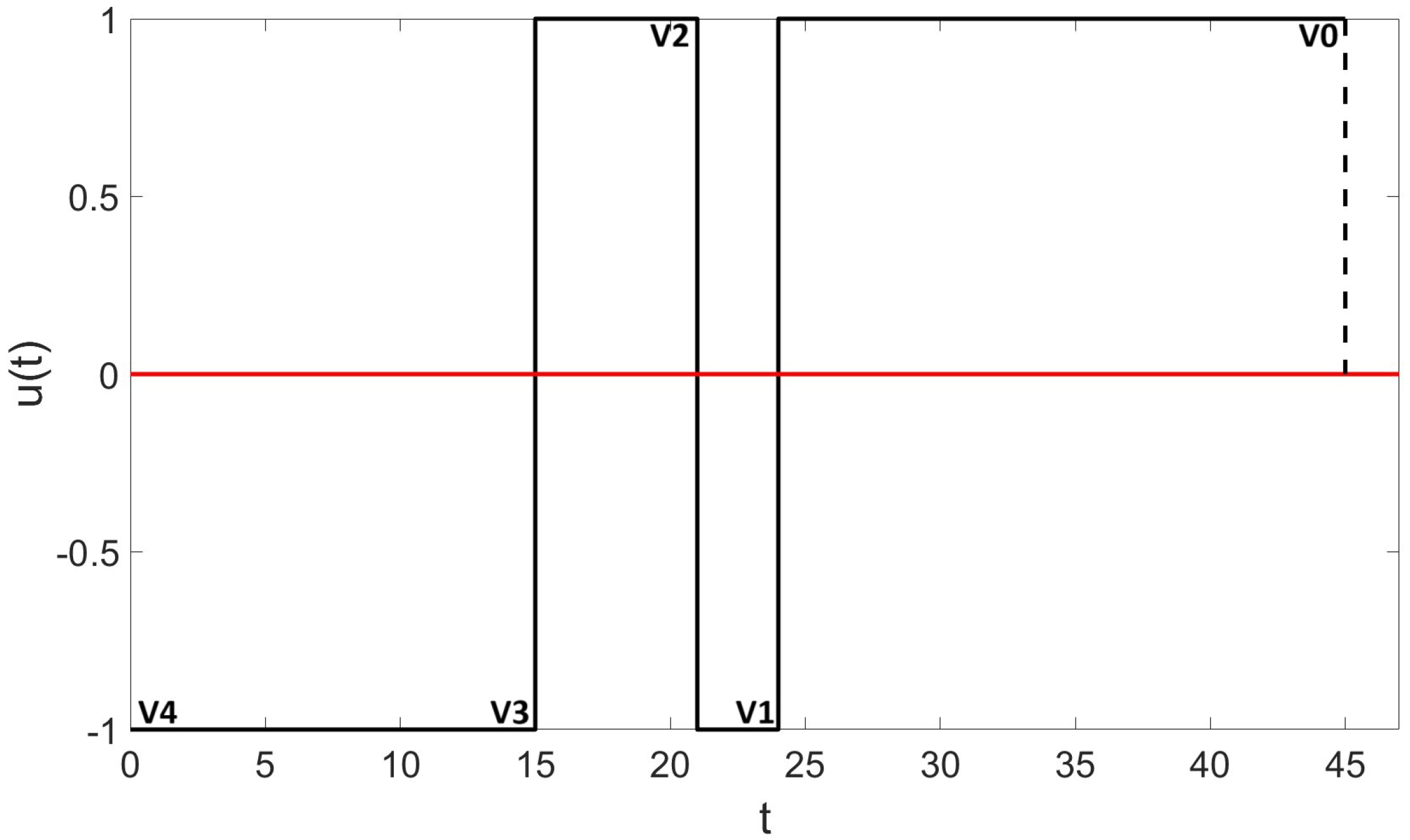
Figure 1. Sample torque profile for i = 1 (single flexible mode), number of switches is 2 i + 1 = 3.
Mathematics 13 01144 g001
Figure 2. Minimum-time optimal control in presence of the process noise using the optimization plan presented in Problem (15). The angular units are either degree (position) or degree/s (velocity). Additionally, the unit of the torque (u(t)) is N.m.
Mathematics 13 01144 g002
Figure 3. The minimum-time optimal control torque profile (i.e., the torque profile shown in Figure 2) is used for w = −3.5, 0 and +3.5. In this figure w = 0 is plotted in black and w = −3.5 and +3.5 are plotted in red and green, respectively. The units are either degree (position) or degree/s (velocity).
Mathematics 13 01144 g003
Figure 4. Phase-plane plots related to the rigid body and flexible mode are shown for the three values of w. The units are either degree (position) or degree/s (velocity). Similar to the previous figure, in this figure w = 0 is plotted in black and w = −3.5 and +3.5 are plotted in red and green, respectively.
Mathematics 13 01144 g004
Table 1. Table showing the simulation values related to the minimum-time control under the influence of the process noise. Note that the angular units are either degree (position) or degree/s (velocity). Additionally, time units are in seconds.
v θ 1 , ( d 1 ) θ 2 , ( d 1 ) θ ˙ 1 , ( d 1 ) θ ˙ 2 , ( d 1 ) t ( v ) ( v 1 ) , ( d 1 )
418000016.4859
393.22462.3465−11.27580.92910.4921
288.21802.1068−9.4138−2.04211.2450
176.1590−0.2394−10.7210−1.049314.0675
0 6.6356 × 10 5 4.9436 × 10 4 5.6409 × 10 5 5.4007 × 10 5 NA
Table 2. Table showing the simulation values related to the minimum-time control under the influence of the process noise at t f , ( d 1 ) . Note that the units are either degree (position) or degree/s (velocity).
w θ 1 , 0 , ( d 1 ) θ 2 , 0 , ( d 1 ) θ ˙ 1 , 0 , ( d 1 ) θ ˙ 2 , 0 , ( d 1 )
−3.5−17.55700.0044−1.00600.0779
0 6.6356 × 10 5 4.9436 × 10 4 5.6409 × 10 5 5.4007 × 10 5
+3.517.5570−0.00341.0059−0.0778
Table 3. Analysis of the impact of each variance on four angular terms. Note that i = 1 , 2 , 3 , 4 .
i θ 0 , ( d 1 ) Ω i 1 Ω i 2 Ω i 3 Ω i 4
1 θ 1 , 0 , ( d 1 ) 0.011880.793930.003000.19119
2 θ ˙ 1 , 0 , ( d 1 ) 00.794500.002030.20347
3 θ 2 , 0 . ( d 1 ) 000.598340.40166
4 θ ˙ 2 , 0 . ( d 1 ) 000.968930.03107
Disclaimer/Publisher’s Note: The statements, opinions and data contained in all publications are solely those of the individual author(s) and contributor(s) and not of MDPI and/or the editor(s). MDPI and/or the editor(s) disclaim responsibility for any injury to people or property resulting from any ideas, methods, instructions or products referred to in the content.