Dynamics of a Class of Chemical Oscillators with Asymmetry Potential: Simulations and Control over Oscillations ^†

Abstract

The literature devoted to the issue of a forced modified Van der Pol–Duffing oscillator with asymmetric potential is a major and varied way to represent nonlinear dissipative chemical dynamics. It is known that this model is based on the real reaction–kinetic scheme. In this paper, we suggest a novel class of oscillators that are appealing to users due to their numerous free parameters and asymmetric potential. The rationale for this is because an expanded model is put out that enables the investigation of both classical and more recent models that have been reported in the literature at a “higher energy level”. We present a few specific modules for examining these oscillators’ behavior. A much broader Web-based application for scientific computing will incorporate this as a key component. Probabilistic construction to offer possible control over the oscillations is also considered.

1. Introduction

The freedom of a potential well may be guaranteed by a number of oscillatory natural phenomena that arise in a range of fields, including chemistry, mechanics, quantum optics, acoustics, hydrodynamics, electronics, and engineering. These phenomena are represented by a general nonlinear oscillator model. Non-equilibrium phenomena like oscillations, bi-stability, complex oscillations, and quasi-chaotic behavior of the reaction have been discovered through investigations of chemical oscillating reactions in a continuously stirred tank reactor (CSTR) [1,2,3,4,5,6,7,8].

In the biological sciences, ecology, demographics, chemistry, social sciences, and other fields, growth models are frequently employed to model a variety of processes. Typically, a system of ODEs is used to create dynamic growth models. Understanding the model’s physics-chemical meaning is helpful in selecting an appropriate growth model. In many cases, a reaction network that potentially triggers the dynamical growth model via mass action kinetics is the ideal way to present this meaning. Such reaction networks are well known for a number of growth models.

Ref. [9] examines the use of a forced modified Van der Pol–Duffing oscillator with asymmetric potential to model nonlinear dissipative chemical dynamics:

$$\left\{\begin{array}{ccc}{\displaystyle \frac{\mathrm{d}x}{\mathrm{d}t}}\hfill & =& y\hfill \\ {\displaystyle \frac{\mathrm{d}y}{\mathrm{d}t}}\hfill & =& -\alpha x-\gamma x^3-\beta +ϵ\left(-\mu (1-x^2)y+Ecos\left(\omega t\right)\right),\hfill \end{array}\right.$$

(1)

where $ϵ$ is a small parameter that describes how small the forced and dissipative terms are. Without going into details, it is known that this model is based on the following reaction–kinetic scheme:

$$\begin{array}{ccc}A\hfill & \stackrel{k_1}{⟶}\hfill & U\hfill \\ B+U\hfill & \stackrel{k_2}{⟶}\hfill & 2U\hfill \\ D+U\hfill & \stackrel{k_3}{⟶}\hfill & Products\hfill \\ U\hfill & \stackrel{k_4}{⟶}\hfill & U^{\prime }\hfill \\ B+U\hfill & \stackrel{k_5}{⟶}\hfill & V\hfill \\ V\hfill & \stackrel{k_6}{⟶}\hfill & U^{\prime }+Products.\hfill \end{array}$$

We will only note that its explicit form is obtained using certain mathematical transformations and application of laws of mass action. For some details, see [1,3,10,11].

The bounds of the domains where Melnikov’s chaos manifests in chemical oscillations are analytically determined using the Melnikov method. There is a substantial amount of varied literature on this topic. We refer the reader to [12,13,14,15,16], where they can locate more relevant research.

Ref. [17] (also see [18]) examines chaos, coexisting attractors, and chaos control in a nonlinear dissipative chemical oscillator.

More precisely, the authors consider the following model [17]:

$$\left\{\begin{array}{ccc}{\displaystyle \frac{\mathrm{d}x}{\mathrm{d}t}}\hfill & =& y\hfill \\ {\displaystyle \frac{\mathrm{d}y}{\mathrm{d}t}}\hfill & =& -\alpha x-\gamma x^3-\beta +ϵ\left(-\mu (1-x^2-k_{1}xy-k_2{y}^2)y+fcos\left(\omega t\right)\right).\hfill \end{array}\right.$$

(2)

In certain instances, after calculating the Melnikov functions, researchers discover that the homo-clinic orbits are so complicated that the formulations of the Melnikov functions cannot be solved analytically. Numerical algorithms are typically suggested and applied for this aim.

In this paper, we propose an oscillator model based on the differential model discussed above. Investigations in light of Melnikov’s approach [19] is considered. A number of simulations are created. Furthermore, we present a few specific modules for examining the dynamics of these fictitious oscillators. The obtained results can be included into a much broader scientific computing application; see [20] for additional information.

Other generalizations of differential models based on the research indicated in the already cited articles [1,2,3,4,5,6,7,8,9,10,11,12,13,14,15,16,17,18] can be obtained with the methodology set forth in the present article and can be considered as real models corresponding to K-angle, N-step reaction-kinetic schemes, and other chemical and biochemical networks [21,22,23,24,25]. In the cited monographs, the reader can find related literature. We will also note some interesting articles published over the years in the authoritative J of Math Chem [26,27,28,29], MATCH Commun Math Comput Chem [30,31], BMC Syst. Biol. [32,33], Biomath [34,35], Math Methods Appl Sci [36], SIAM J Appl Math [37], Biomath Communications [38], J Amer Chem Soc [39], Mathematics [40], and other specialized journals.

The following is this paper’s plan. In Section 2, we present our new model. Section 3 presents a few simulations. A new modified hypothetical model is considered in Section 4. Possible control over oscillations and approximation with restrictions is considered in Section 4.1. Section 4.2 also examines probabilistic construction as a potential means of controlling the oscillations. Section 5 brings us to a close.

2. The New Model

We explore the next new class of oscillators

$$\left\{\begin{array}{ccc}{\displaystyle \frac{\mathrm{d}x}{\mathrm{d}t}}\hfill & =& y\hfill \\ {\displaystyle \frac{\mathrm{d}y}{\mathrm{d}t}}\hfill & =& -\alpha x-\gamma x^3-\beta +ϵ\left(-\mu y+{\displaystyle \sum _{j=1}^N}{g}_{j}cos\left(j\omega t\right)\right),\hfill \end{array}\right.$$

(3)

where $0\le ϵ<1$, $\mu >0$, $g_i\ge 0,i=1,2,\dots ,N$, and N is positive integer.

The associated Hamiltonian ($ϵ=0$) is ${\displaystyle \frac{1}{2}}{y}^2+\beta x+{\displaystyle \frac{1}{2}}\alpha x^2+{\displaystyle \frac{1}{4}}\gamma x^4$. The homo-clinic orbit leads to the equilibrium points of system is given by [9]

$$\begin{array}{c}{x}_0\left(t\right)=\overline{x}+{\displaystyle \frac{\sqrt{2}{\sigma }^2}{\gamma (\overline{x}\pm \delta \cosh \left(\sigma t\right))}},\hfill \\ y_0\left(t\right)=\mp {\displaystyle \frac{\sqrt{2}\delta {\sigma }^3}{\gamma }}{\displaystyle \frac{\sinh \left(\sigma t\right)}{{(\overline{x}\pm \delta \cosh \left(\sigma t\right))}^2}},\hfill \end{array}$$

(4)

where

$${\sigma }^2={\displaystyle \frac{-2\alpha -3\gamma {\overline{x}}^2}{2}};{\delta }^2={\displaystyle \frac{-2\alpha -\gamma {\overline{x}}^2}{2\gamma }};\overline{x}=-{\displaystyle \frac{\beta }{2\alpha }}\sqrt{{\displaystyle \frac{-3\gamma }{\alpha }}}.$$

Some details can be found in [9]. The homo-clinic orbit for $\alpha =-1;\gamma =1/3;\beta =1/2$ is depicted in Figure 1. Energy potential is depicted in Figure 2.

Considerations in the Light of Melnikov’s Approach

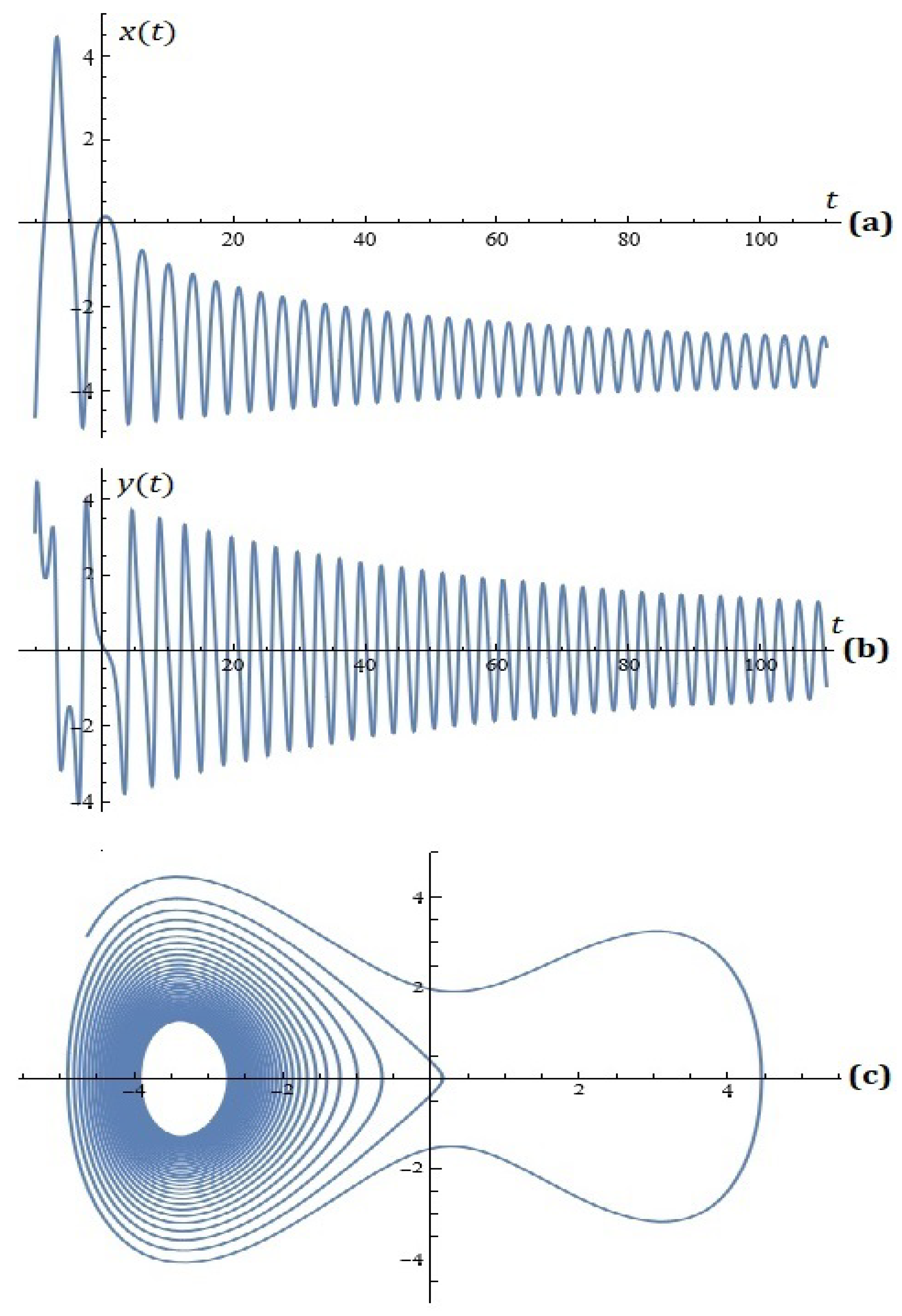
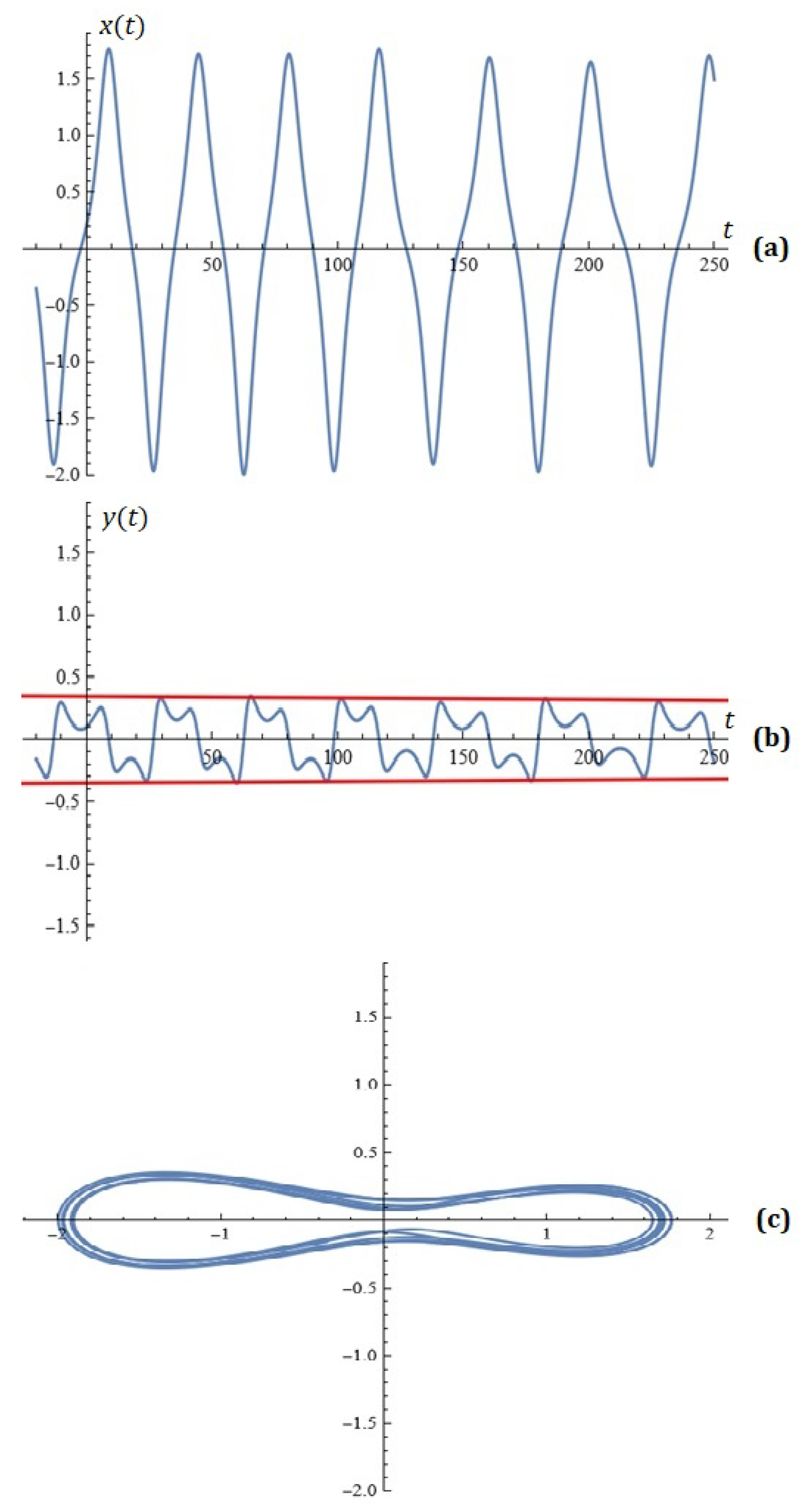
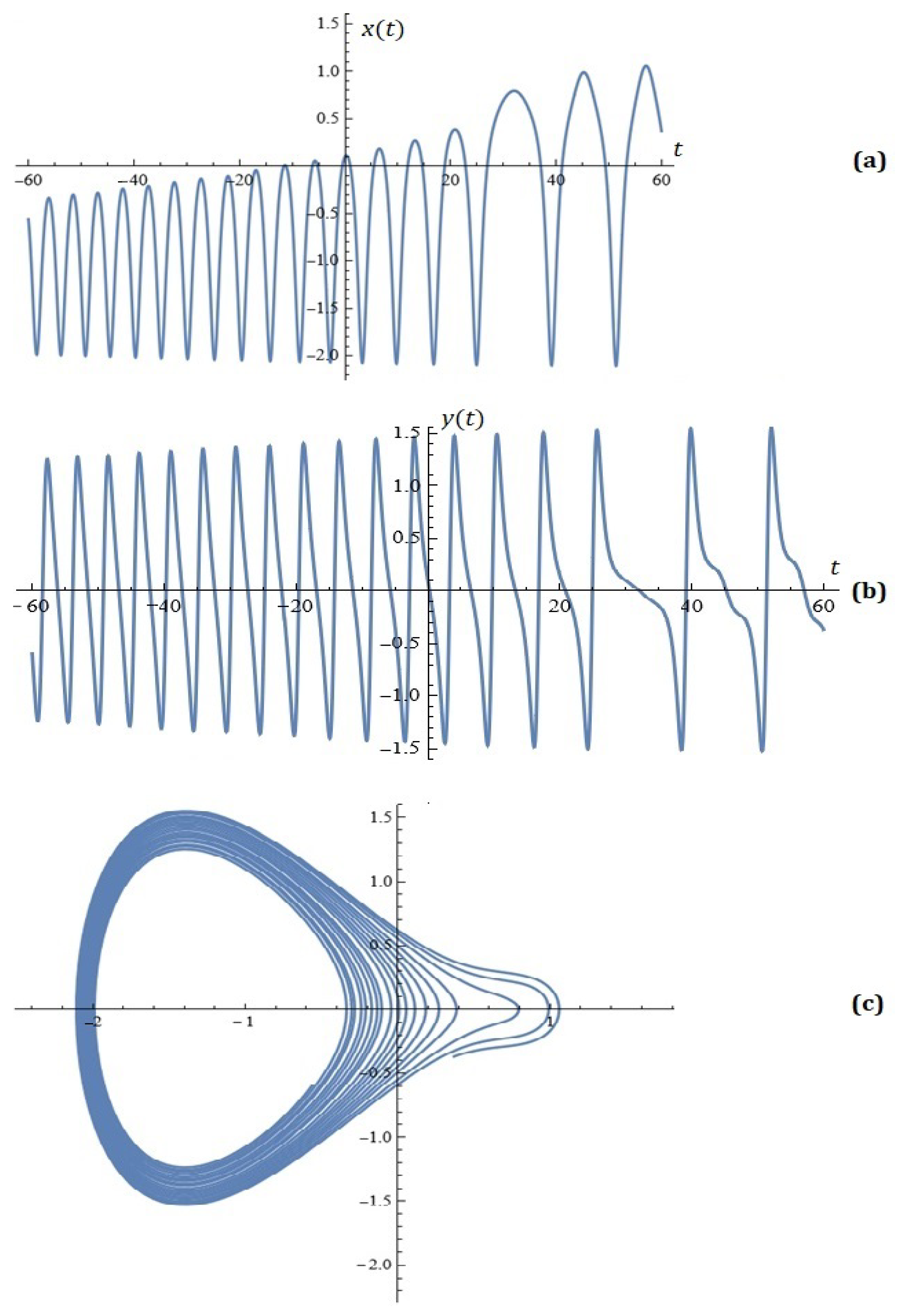
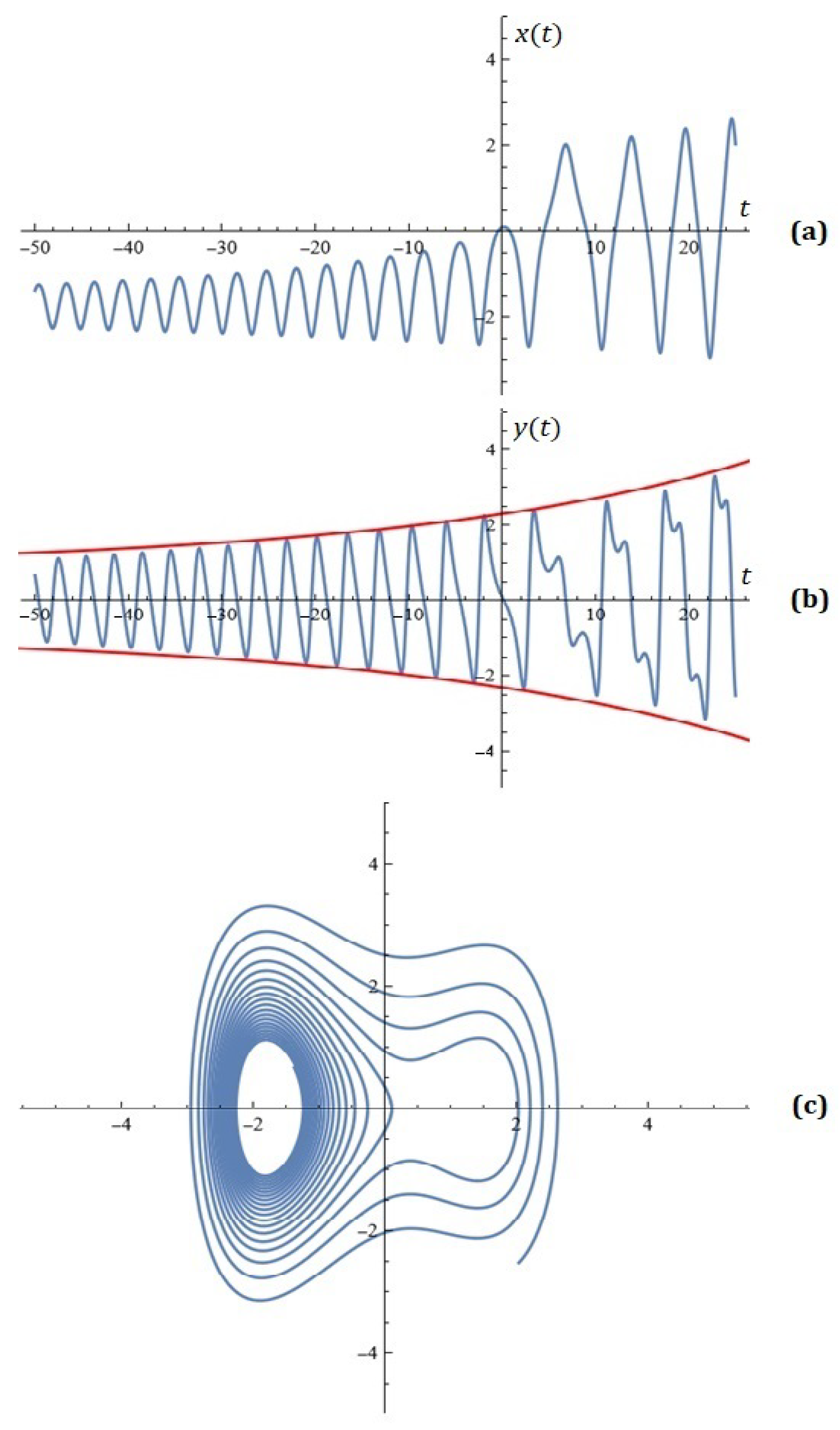
When $ϵ\ne 0$, the Melnikov function provides a measure of the leading-order distance between the stable and unstable manifolds, which may be used to determine the transverse intersection of the stable and unstable manifolds.

By definition, the integral of Melnikov corresponding to new model (3) is given by

$$M\left(t_0\right)={\displaystyle {\int }_{-\infty }^{\infty }}\left(-\mu y_0^2\left(t\right)+y_0\left(t\right){\displaystyle \sum _{j=1}^N}{g}_{j}cos\left(j\omega (t+t_0)\right)\right)\mathrm{d}t,$$

(5)

where the function $y_0\left(t\right)$ is defined by Equation (4).

The task of determining the root of $M\left(t_0\right)$ is more intriguing from a numerical perspective because the parameters that appear in the suggested differential model are subject to certain practical and physical constraints. It is well known that chaos arises if $M\left(t_0\right)=0$ and ${\displaystyle \frac{\mathrm{d}M\left(t_0\right)}{\mathrm{d}{t}_0}}\ne 0$ for some $t_0$ and some sets of parameters.

In the particular case $N=1$ (partially known result) for the Melnikov function $M\left(t_0\right)$, we have

$$M\left(t_0\right)=-\mu {\displaystyle \frac{2{\delta }^2{\sigma }^6}{{\gamma }^2}}{J}_1\mp {\displaystyle \frac{\sqrt{2}\delta {\sigma }^3}{\gamma }}{g}_{1}sin\left(\omega t_0\right)J_2,$$

(6)

where

$$J_1={\displaystyle {\int }_{-\infty }^{\infty }}{\displaystyle \frac{{\sinh }^2\left(\sigma t\right)}{{(\overline{x}\pm \delta \cosh \left(\sigma t\right))}^4}}\mathrm{d}t$$

and

$$J_2={\displaystyle {\int }_{-\infty }^{\infty }}{\displaystyle \frac{\sinh \left(\sigma t\right)sin\left(\omega t\right)}{{(\overline{x}\pm \delta \cosh \left(\sigma t\right))}^2}}\mathrm{d}t.$$

Remark 1.

We will explicitly note that our research essentially uses the methodology proposed in [9] (see also [12]). Below, we place some expressions for the indicated integrals with the sole purpose of eliminating some unintentional technical errors made in some of the publications already cited.

Using substitution $\sigma t=\tau$, we find

$$J_1={\displaystyle \frac{1}{\sigma }}{\displaystyle {\int }_{-\infty }^{\infty }}{\displaystyle \frac{{\sinh }^2\left(\tau \right)}{{(\overline{x}\pm \delta \cosh \left(\tau \right))}^4}}\mathrm{d}\tau ,$$

$$J_2={\displaystyle \frac{1}{\sigma }}{\displaystyle {\int }_{-\infty }^{\infty }}{\displaystyle \frac{\sinh \left(\tau \right)sin\left(\frac{\omega }{\sigma }\tau \right)}{{(\overline{x}\pm \delta \cosh \left(\tau \right))}^2}}\mathrm{d}\tau .$$

Following the ideas from articles [9,10,11,12], let us denote $\pm {\displaystyle \frac{\delta }{\overline{x}}}={\displaystyle \frac{\sqrt{{\eta }^2-1}}{\eta }}$. Then,

$$J_1={\displaystyle \frac{2{\eta }^4}{\sigma {\overline{x}}^4}}{\displaystyle {\int }_0^{\infty }}{\displaystyle \frac{{\sinh }^2\left(\tau \right)}{{(\eta +\sqrt{{\eta }^2-1}\cosh \left(\tau \right))}^4}}\mathrm{d}\tau .$$

Using (see integrals table [41]) for integral $J_1$ become

$$J_1=-{\displaystyle \frac{{\eta }^4}{3\sigma {\overline{x}}^4\sqrt{{\eta }^2-1}}}{Q}_2^1\left(\eta \right),$$

where $Q_2^1(.)$ is associated Legendre function of the second kind (see [41,42]) defined by

$$Q_{\nu }^{\theta }\left(\kappa \right)={\displaystyle \frac{e^{i\theta \pi }\Gamma (\nu +\theta +1)\Gamma \left(\frac{1}{2}\right)}{2^{\nu +1}\Gamma (\nu +\frac{3}{2})}}{({\kappa }^2-1)}^{{\displaystyle \frac{\theta }{2}}}{\kappa }^{-\nu -\theta -1}{\times }_2{F}_1\left({\displaystyle \frac{\nu +\theta +2}{2}},{\displaystyle \frac{\nu +\theta +1}{2}},\nu +{\displaystyle \frac{3}{2}},\kappa \right),$$

where $\Gamma (.)$ is the Gamma function, and ₂$F_1(.,.,.,.)$ is the hyper-geometric function.

Using residue theorem for integral $J_2$ we obtain (for some details see [9]):

$$J_2=\mp {\displaystyle \frac{\pi \omega \delta {\sigma }^2}{\alpha {\overline{x}}^{4}15\sqrt{\frac{-\alpha }{\gamma }}}}{\displaystyle \frac{1}{\left(1+\frac{\sqrt{2}}{{(-\alpha )}^{\frac{3}{2}}}\left(\frac{3\pi }{4}-\frac{1}{\sqrt{-\alpha }}\tanh \left(\frac{\pi }{2\sqrt{-\alpha }}\right)\right)\right)}}{\times }_2{F}_1({\displaystyle \frac{5}{2}},2,{\displaystyle \frac{7}{2}},\eta ).$$

The appearance of horseshoe chaos can be derived from (6) after substituting the thus obtained explicit representations for the integrals $J_1$ and $J_2$ and examining the nonlinear equation $M\left(t_0\right)=0$.

Remark 2.

Melnikov’s criterion for the occurrence of the intersection between the disturbed and unperturbed separatrices for a fixed N can be formulated by the reader.

Because it is described in terms of gamma and hypergeometric functions, the explicit representation of $M\left(t_0\right)$ in this instance (as well as that for large values of the parameter N) is time-consuming.

This requires the user to perform a number of preparatory operations on the integrals $J_j$ and described above before using specialized modules implemented in existing computer–algebraic systems for scientific research.

Before that, it is convenient to use the following representation:

$$cos\left(i\omega (t+t_0)\right)=cos\left(i\omega t\right)cos\left(i\omega t_0\right)-sin\left(i\omega t\right)sin\left(i\omega t_0\right)$$

when calculating the integral (5).

Investigations in the light of Melnikov’s approach is considered for some extended differential models (see [43,44]).

Numerical methods for solving nonlinear equations can be found in [45,46,47,48,49,50,51].

3. Some Simulations

We will concentrate on a few intriguing simulations here:

Example 1.

For given $\alpha =-1;\beta =0.5;\gamma =0.33;\mu =1.03;N=2;ϵ=0.0095;\omega =1;g_1=0.1;g_2=0.4$, the simulations on the system (3) for $x_0=0.1$; $y_0=0.1$ are depicted in Figure 3.

Example 2.

For given $\alpha =-1.2;\beta =0.3;\gamma =0.81;\mu =0.1;N=3;ϵ=0.0095;\omega =1;$ $g_1=0.1;$ $g_2=0.4;g_3=0.2$, the simulations on the system (3) for $x_0=0.1$; $y_0=0.1$ are depicted in Figure 4.

Example 3.

For given $\alpha =-2.1;\beta =0.6;\gamma =0.2;\mu =1.3;N=4;ϵ=0.0095;$ $\omega =1.1;$ $g_1=0.05;g_2=0.1;g_3=0.05;g_4=0.1$, the simulations on the system (3) for $x_0=0.1$; $y_0=0.1$ are depicted in Figure 5.

4. The New Modified Model

We consider the following new class of modified oscillators:

$$\left\{\begin{array}{ccc}{\displaystyle \frac{\mathrm{d}x}{\mathrm{d}t}}\hfill & =& y\hfill \\ {\displaystyle \frac{\mathrm{d}y}{\mathrm{d}t}}\hfill & =& -\alpha x-\gamma x^3-\beta +ϵ\left(-{\mu y\left|y\right|}^{p-1}+{\displaystyle \sum _{j=1}^N}{g}_{j}cos\left(j\omega t\right)\right),\hfill \end{array}\right.$$

(7)

where $0\le ϵ<1$, $\mu >0$, $g_i\ge 0,i=1,2,\dots ,N$, N is positive integer, and natural number $p\ge 1$ is the damping exponent.

The dynamics of this differential model in the light of Melnikov’s considerations can be conducted with the apparatus proposed in this article and many publications that we have indicated in the cited bibliographic reference.

We will skip that analysis here. We will consider only two characteristic examples illustrating the dynamics of the new model (7).

Example 4.

For given $\alpha =-2.1;\beta =0.6;\gamma =0.2;\mu =1.3;N=5;p=2;$ $ϵ=0.0095;$ $\omega =1.1;g_1=0.05;g_2=0.1;g_3=0.05;g_4=0.1;g_5=0.2$, the simulations on the system (7) for $x_0=0.1$; $y_0=0.2$ are depicted in Figure 6.

Example 5.

For given $\alpha =-0.3;\beta =0.4;\gamma =0.03;\mu =0.8;N=6;p=4;ϵ=0.0095;$ $\omega =1.2;$ $g_1=0.4;g_2=0.1;g_3=0.05;g_4=0.1;g_5=0.2;g_6=0.4$, the simulations on the system (7) for $x_0=0.1$; $y_0=0.1$ are depicted in Figure 7.

Example 6.

For given $\alpha =-0.08;\beta =0.01;\gamma =0.05;\mu =0.9;N=8;p=6;ϵ=0.0095;$ $\omega =0.05;$ $g_1=0.4;g_2=0.1;g_3=0.1;g_4=0.1;g_5=0.1;g_6=0.1;g_7=0.1;g_8=0.2$, the simulations on the system (7) for $x_0=0.2$; $y_0=0.1$ are depicted in Figure 8.

4.1. Potential Oscillation Control: Approximation with Limitations

For instance, the new model (7) offers a user-preset level (or fork) for the oscillations of the y component of the differential system solution, making it appealing for engineering computations due to its abundance of free parameters.

Suppose the given constraint or fork $\left(F\right(t),-F(t\left)\right)$ is of the type (most common constraint)

$$F\left(t\right)=a_1+{\displaystyle \frac{a_2}{1+a_3{e}^{a_{4}kt}}}.$$

(8)

We shall state clearly that the problem was primarily solved using traditional optimization approaches (in Example 5, see in Figure 7b how the function $F\left(t\right)$ is of the form: $F\left(t\right)=-0.2-{\displaystyle \frac{3}{1+0.5e^{0.01t}}}$) and we will not dwell on them here.

With user-fixed values of $N=8$, $p=6$ and the function $F\left(t\right)=-0.25-{\displaystyle \frac{0.15}{1+0.5e^{0.0375t}}}$, the desired control over oscillations is achieved for the parameters given in Example 6 (see Figure 8b).

In certain situations (due to strictly mechanical and physical limitations), the function $F\left(t\right)$ may be of the log–logistic, “cut”, “U- and S-shaped”, or “activation” function type.

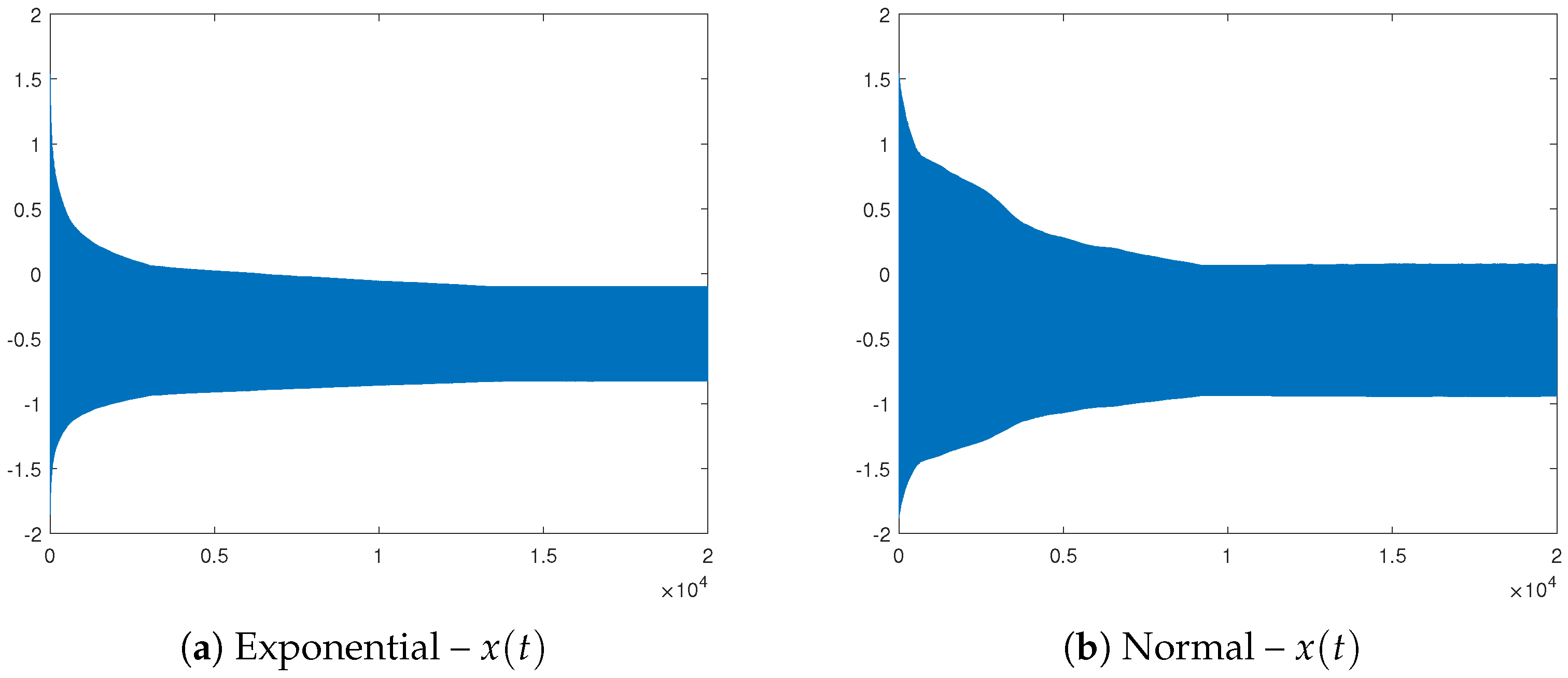
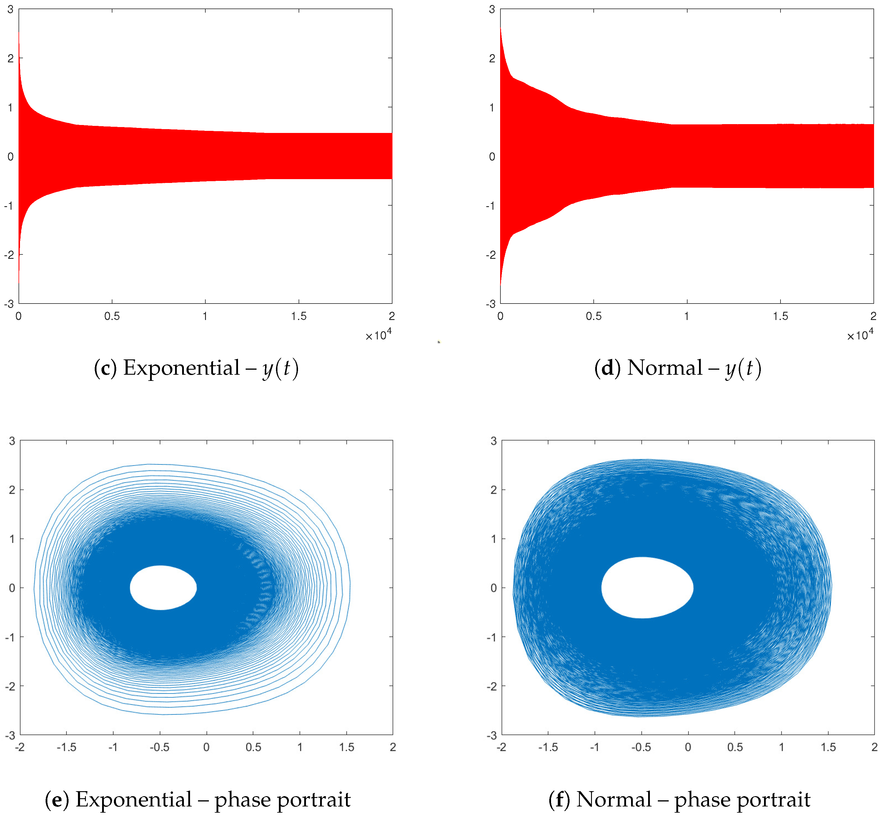
4.2. Probabilistic Construction to Possible Control over the Oscillations

The job of creating a probabilistic structure in order to potentially control the oscillations of the dynamic model suggested in this article is very intriguing. Note that we can assume without loss of generalization that ${\sum }_{j=1}^N{g}_j=1$ and thus we can view the coefficients $g_j$ as the probabilities for some random variable, say $\xi$, stated on the domain $\left\{1,2,\cdots ,N\right\}$. Denote its characteristic function by $\Psi \left(x\right)$ and by $\mathbb{E}$ the mathematical expectation with regard to the corresponding probability low. Thus, using the exponential presentation of the cos-function

$$cos\left(x\right)={\displaystyle \frac{e^{ix}+e^{-ix}}{2}},$$

(9)

we rewrite the y-term of dynamics (7) as

$$\begin{array}{cc}\hfill {\displaystyle \frac{\mathrm{d}y}{\mathrm{d}t}}& =-\alpha x-\gamma x^3-\beta +ϵ\left(-\mu y{\left|y\right|}^{p-1}+\sum _{j=1}^N{g}_j{\displaystyle \frac{e^{ij\omega t}+e^{-ij\omega t}}{2}}\right)\hfill \\ \hfill & =-\alpha x-\gamma x^3-\beta +ϵ\left(-\mu y{\left|y\right|}^{p-1}+{\displaystyle \frac{\mathbb{E}\left[e^{i\omega t\xi }\right]+\mathbb{E}\left[e^{-i\omega t\xi }\right]}{2}}\right)\hfill \\ \hfill & =-\alpha x-\gamma x^3-\beta +ϵ\left(-\mu y{\left|y\right|}^{p-1}+{\displaystyle \frac{\Psi \left(\omega t\right)+\Psi \left(-\omega t\right)}{2}}\right).\hfill \end{array}$$

(10)

This presentation indicates that the restriction that the distribution is stated on the domain $\left\{1,2,\dots ,N\right\}$ is not essential. On the other hand, if the probability distribution is stated on an arbitrary domain—say, D—then dynamics (10) still hold. Note that its original form has to be defined as

$${\displaystyle \frac{\mathrm{d}y}{\mathrm{d}t}}=-\alpha x-\gamma x^3-\beta +ϵ\left(-\mu y{\left|y\right|}^{p-1}+\underset{D}{\int }cos\left(u\omega t\right)g\left(\mathrm{d}u\right)\right).$$

(11)

For a fixed value $p=1$, Melnikov function (5) turns into

$$\begin{array}{c}\hfill M\left(t_0\right)=\underset{-\infty }{\overset{\infty }{\int }}\left(-\mu y_0^2\left(t\right)+y_0\left(t\right)\sum _{j=1}^N{g}_{j}cos\left(j\omega \left(t+t_0\right)\right)\right)\mathrm{d}t\\ \hfill =\underset{-\infty }{\overset{\infty }{\int }}\left(-\mu y_0^2\left(t\right)+y_0\left(t\right){\displaystyle \frac{\Psi \left(\omega \left(t+t_0\right)\right)+\Psi \left(-\omega \left(t+t_0\right)\right)}{2}}\right)\mathrm{d}t.\end{array}$$

(12)

Let us consider some particular cases. First, suppose that the random variable $\xi$ is distributed under the exponential low with intensity $\lambda$. Its domain is the positive real half-line $D={\mathbb{R}}^{+}$, the density is $g\left(x\right)=\lambda e^{\lambda x}$, and the characteristic function is

$$\Psi \left(x\right)={\displaystyle \frac{\lambda }{\lambda -ix}}.$$

(13)

Having in mind the relation

$$\Psi \left(x\right)+\Psi \left(-x\right)=2{\displaystyle \frac{{\lambda }^2}{{\lambda }^2+x^2}},$$

(14)

we rewrite y-dynamics (10) as

$${\displaystyle \frac{\mathrm{d}y}{\mathrm{d}t}}=-\alpha x-\gamma x^3-\beta +ϵ\left(-\mu y{\left|y\right|}^{p-1}+{\displaystyle \frac{{\lambda }^2}{{\lambda }^2+{\omega }^2{t}^2}}\right).$$

(15)

The Melnikov function (12) for $p=1$ turns into

$$M\left(t_0\right)=\underset{-\infty }{\overset{\infty }{\int }}\left(-\mu y_0^2\left(t\right)+y_0\left(t\right){\displaystyle \frac{{\lambda }^2}{{\lambda }^2+{\omega }^2{\left(t+t_0\right)}^2}}\right)\mathrm{d}t.$$

(16)

Some simulations based on this distribution are depicted in Figure 9a,c,e. The used parameters are as follows: $\alpha =1$, $\beta =0.6$, $\gamma =0.85$, $ϵ=0.01$, $\mu =0.1$, $\omega =2$, $p=5$, and $\lambda =0.1$.

Let us provide a second example based on the important $\left(q,\sigma \right)$-Gaussian distribution. Let us remind that its characteristic function is

$$\Psi \left(x\right)=e^{iqx-{\displaystyle \frac{{\sigma }^2{x}^2}{2}}}.$$

(17)

Thus, having in mind the relation

$$\Psi \left(x\right)+\Psi \left(-x\right)=2e^{-{\displaystyle \frac{{\sigma }^2{x}^2}{2}}}cos\left(qx\right),$$

(18)

we obtain for the y-dynamics (10)

$${\displaystyle \frac{\mathrm{d}y}{\mathrm{d}t}}=-\alpha x-\gamma x^3-\beta +ϵ\left(-\mu y{\left|y\right|}^{p-1}+e^{-{\displaystyle \frac{{\sigma }^2{\omega }^2{t}^2}{2}}}cos\left(q\omega t\right)\right).$$

(19)

Hence, the Melnikov function (12) for $p=1$ turns into

$$M\left(t_0\right)=\underset{-\infty }{\overset{\infty }{\int }}\left(-\mu y_0^2\left(t\right)+y_0\left(t\right)e^{-{\displaystyle \frac{{\sigma }^2{\omega }^2{\left(t+t_0\right)}^2}{2}}}cos\left(q\omega \left(t+t_0\right)\right)\right)\mathrm{d}t.$$

(20)

The dynamics as well as the phase portrait are presented in Figure 9b,d,f. We use the standard Gaussian distribution, i.e., $q=0$ and $\sigma =1$. All other parameters are the same except the perturbation term—we consider now $ϵ=0.001$.

5. Concluding Remarks

In this study, we investigated a new hypothetical differential model with many free parameters, which makes it user-friendly.

We introduce some particular modules for studying the behavior of these oscillators.

Some of them include a cloud version that just needs an internet connection and a browser.

This will be a key part of a much larger scientific computing Web-based application that is being developed.

1. Using a forced modified Van der Pol–Duffing oscillator with an asymmetric potential to describe nonlinear dissipative chemical dynamics (reviewed in [9]) can be carried out at a higher energy level by considering the following generalized differential model:

$$\left\{\begin{array}{ccc}{\displaystyle \frac{\mathrm{d}x}{\mathrm{d}t}}\hfill & =& y\hfill \\ {\displaystyle \frac{\mathrm{d}y}{\mathrm{d}t}}\hfill & =& -\alpha x-\gamma x^3-\beta +ϵ\left(-\mu (1-x^2)y+{\displaystyle \sum _{j=1}^N}{g}_{j}cos\left(j\omega t\right)\right),\hfill \end{array}\right.$$

(21)

where $g_i>0,i=1,2,\dots ,N$.

2. The reader can also formulate and explore the following generalization of model (2):

$$\left\{\begin{array}{ccc}{\displaystyle \frac{\mathrm{d}x}{\mathrm{d}t}}\hfill & =& y\hfill \\ {\displaystyle \frac{\mathrm{d}y}{\mathrm{d}t}}\hfill & =& -\alpha x-\gamma x^3-\beta +ϵ\left(-\mu (1-x^2-k_{1}xy-k_2{y}^2)y+{\displaystyle \sum _{j=1}^N}{g}_{j}cos\left(j\omega t\right)\right).\hfill \end{array}\right.$$

(22)

We will consider only two characteristic examples illustrating the dynamics of the new model (21).

Example 7.

For given $\alpha =-1;\beta =0.5;\gamma =0.7;\mu =1.3;N=3;ϵ=0.0095;$ $\omega =1;$ $g_1=0.1;g_2=0.4;g_3=0.2$, the simulations on the system (21) for $x_0=0.1$; $y_0=0.1$ are depicted in Figure 10.

Example 8.

For given $\alpha =-2.1;\beta =0.6;\gamma =0.2;\mu =1.3;N=4;ϵ=0.0095;$ $\omega =1.1;$ $g_1=0.05;g_2=0.1;g_3=0.05;g_4=0.1$, the simulations on the system (21) for $x_0=0.1$; $y_0=0.1$ are depicted in Figure 11.

With user-fixed $N=4$, and the function $F\left(t\right)$ of the exponential type

$$F\left(t\right)=-2.5-1.9{\displaystyle e^{0.0942t}}$$

the desired control over oscillations is achieved for the parameters given in Example 8 (see Figure 11b).

Finally, let us mention that the approach for controlling the oscillations suggested in Section 4.2 can be applied to the generalizations (21) and (22) too. The respective y-dynamics turn into

$$\begin{array}{cc}\hfill {\displaystyle \frac{\mathrm{d}y}{\mathrm{d}t}}& =-\alpha x-\gamma x^3-\beta +ϵ\left(-\mu \left(1-x^2\right)y+{\displaystyle \frac{\Psi \left(\omega t\right)+\Psi \left(-\omega t\right)}{2}}\right),\hfill \\ \hfill {\displaystyle \frac{\mathrm{d}y}{\mathrm{d}t}}& =-\alpha x-\gamma x^3-\beta +ϵ\left(-\mu \left(1-x^2-k_{1}xy-k_2{y}^2\right)y+{\displaystyle \frac{\Psi \left(\omega t\right)+\Psi \left(-\omega t\right)}{2}}\right).\hfill \end{array}$$

(23)

For completeness, we will consider another simulation on the new differential model (22) proposed above.

Example 9.

For given $\alpha =-1.9;\beta =0.7;\gamma =0.7;\mu =1.1;N=4;ϵ=0.0095;$ $\omega =1.12;$ $g_1=0.17;g_2=0.1;g_3=0.18;g_4=0.2;k_1=0.9;k_2=0.6$, the simulations on the system (22) for $x_0=0.1$; $y_0=0.1$ are depicted in Figure 12.

With user-fixed $N=4$, and the function $F\left(t\right)$ of the exponential type

$$F\left(t\right)=-0.9-1.4{\displaystyle e^{0.0261t}}$$

the desired control over oscillations is achieved for the parameters given in Example 9 (see Figure 12b).

In [52], the authors consider the chaotic dynamics of an extended Van der Pol–Duffing system of the type

$$\begin{array}{ccc}{\displaystyle \frac{\mathrm{d}x}{\mathrm{d}t}}\hfill & =& y,\hfill \\ {\displaystyle \frac{\mathrm{d}y}{\mathrm{d}t}}\hfill & =& -ax-b{x}^3-c{x}^5+ϵ\left(\mu (1-x^2)y+fxcos\left(\omega t\right)-dg\left(x\right)\right),\hfill \end{array}$$

(24)

where $a>0,b<0,c>0$ and the damping coefficient, excitation amplitude, disturbance amplitude, and excitation frequency are $\mu >0,f>0,d>0,\omega >0$, respectively; with period $2l$, $g\left(x\right)$ is a non-smooth periodic function of x.

In particular, the following differential model was proposed [52]:

$$\begin{array}{ccc}{\displaystyle \frac{\mathrm{d}x}{\mathrm{d}t}}\hfill & =& y,\hfill \\ {\displaystyle \frac{\mathrm{d}y}{\mathrm{d}t}}\hfill & =& -ax-b{x}^3-c{x}^5+ϵ(\mu (1-x^2)y+fxcos\left(\omega t\right)\hfill \\ \hfill & & -{\displaystyle \frac{2d}{\pi }}(1-2{\displaystyle \sum _{k=1}^{\infty }}{\displaystyle \frac{cos\left(2kx\right)}{4k^2-1}})).\hfill \end{array}$$

(25)

We plan to expand the theoretical basis of this differential system in a future paper by adding new factors to its dynamics, following the idea proposed in this paper, and we will show that this model is based on a real reaction–kinetic scheme.

Specialists working in this scientific direction have the floor.

Our paper is also dedicated to the memory of Prof. Svetoslav Markov (1943–2023), who conducted serious research in the field of reaction kinetics, K-angle, N-step reaction schemes, Bateman chains, etc. We are convinced that some of these studies will serve as the basis for future research in modeling chemical and biochemical oscillators.

As we have already noted, after the brief study of the model in the light of Melnikov’s theory, our main efforts were directed to simulations with the new differential model, which has many degrees of freedom and is thus attractive to researchers. Secondly, we will note the interesting research related to oscillation control (research that is not yet sufficiently well represented in publications dedicated to this topic). In addition to classical methods from the field of approximation theory with constraints (well-known approximation and optimization techniques are essentially used) we offer probabilistic constructions for oscillation control, topics which may be of interest to engineers and specialists working in this scientific field.

References

1. Boissonade, J.; De Kepper, P. Transitions from bistability to limit cycle oscillations. Theoretical analysis and experimental evidence in an open chemical system. J. Phys. Chem. 1980, 84, 501–506. [Google Scholar] [CrossRef]
2. Zhabotinskii, A.M. Biological and Biochemical Oscillators; Academic Press: New York, NY, USA, 1972. [Google Scholar]
3. Epstein, I.R.; Showalter, K. Nonlinear chemical dynamics: Oscillations, patterns, and chaos. J. Phys. Chem. 1996, 100, 13132–13147. [Google Scholar] [CrossRef]
4. Belousov, B.P. Oscillations and Travelling Waves in Chemical Systems; Wiley: New York, NY, USA, 1985. [Google Scholar]
5. Zhabotinsky, A.M.; Buchholtz, F.; Kiyatkin, A.B.; Epstein, I.R. Oscillations and waves in metal-ion-catalyzed bromate oscillating reactions in highly oxidized states. J. Phys. Chem. 1993, 97, 7578–7584. [Google Scholar] [CrossRef]
6. Zhang, D.; Gyorgyi, L.; Peltier, W.R. Deterministic chaos in the Belousov-Zhabotinsky reaction: Experiments and simulations. Chaos 1993, 3, 723–745. [Google Scholar] [CrossRef]
7. Ali, F.; Menzinger, M. Stirring effects and phase-dependent inhomogeneity in chemical oscillations: The Belousov-Zhabotinsky reaction in a CSTR. J. Phys. Chem. A 1997, 101, 2304–2309. [Google Scholar] [CrossRef]
8. Bartuccelli, M.; Gentile, G.; Wright, J.A. Stable dynamics in forced systems with sufficiently high/low forcing frequency. Chaos 2016, 26, 083108. [Google Scholar] [CrossRef] [PubMed]
9. Miwadinou, C.H.; Monwanoua, A.V.; Yovoganc, J.; Hinvia, L.A.; Nwagoum Tuwae, P.R.; Chabi Orou, J.B. Modeling nonlinear dissipative chemical dynamics by a forced modified Van der Pol-Duffing oscillator with asymmetric potential: Chaotic behaviors predictions. Chin. J. Phys. 2018, 56, 1089–1104. [Google Scholar] [CrossRef]
10. Olabode, D.L.; Miwadinou, C.H.; Monwanou, A.V.; Chabi Orou, J.B. Horseshoes chaos and its passive control in dissipative nonlinear chemical dynamics. Phys. Scr. 2018, 93, 085203. [Google Scholar] [CrossRef]
11. Olabode, D.L.; Miwadinou, C.H.; Monwanou, V.A.; Chabi Orou, J.B. Effects of passive hydrodynamics force on harmonic and chaotic oscillations in nonlinear chemical dynamics. Physica D 2019, 386, 49–59. [Google Scholar] [CrossRef]
12. Miwadinou, C.H.; Monwanou, A.V.; Hinvi, A.L.; Koukpemedji, A.A.; Ainamon, C.; Orou, J.B.C. Melnikov chaos in a modified Rayleigh-Duffing oscillator with ϕ6 potential. Int. J. Bifurc. Chaos 2016, 26, 1650085. [Google Scholar] [CrossRef]
13. Ainamon, C.; Miwadinou, C.H.; Monwanou, A.V.; Orou, J.B.C. Analysis of multiresonance and chaotic behavior of the polarization in materials modeled by a duffing equation with multifrequency excitations. Appl. Phys. Res. 2014, 6, 74–86. [Google Scholar] [CrossRef]
14. Miwadinou, C.H.; Monwanou, A.V.; Chabi Orou, J.B. Active control of the parametric resonance in the modified Rayleigh-Duffing oscillator. Afr. Rev. Phys. 2014, 9, 227–235. [Google Scholar]
15. Miwadinou, C.H.; Monwanou, A.V.; Chabi Orou, J.B. Effect of nonlinear dissipation on the basin boundaries of a driven two-well modified rayleigh-duffing oscillator. Int. J. Bifurc. Chaos 2015, 25, 1550024. [Google Scholar] [CrossRef]
16. Miwadinou, C.H.; Hinvi, A.L.; Monwanou, A.V.; Chabi Orou, J.B. Nonlinear dynamics of a ϕ6 modified duffing oscillator: Resonant oscillations and transition to chaos. Nonlinear Dyn. 2017, 88, 97–113. [Google Scholar] [CrossRef]
17. Adechinanm, A.; Kpomahou, Y.; Hinvi, L.; Miwadinou, C. Chaos, coexisting attractors and chaos control in a nonlinear dissipative chemical oscillator. Chin. J. Phys. 2022, 77, 2694–2697. [Google Scholar]
18. Adechinan, J.A.; Kpomahou, Y.J.F.; Miwadinou, C.H.; Hinvi, L.A. Dynamics and active control of chemical oscillations modeled as a forced generalized Rayleigh oscillator with asymmetric potential. Int. J. Basic Appl. Sci. 2021, 10, 20–31. [Google Scholar]
19. Melnikov, V.K. On the stability of a center for time–periodic perturbation. Trans. Mosc. Math. Soc. 1963, 12, 3–52. [Google Scholar]
20. Golev, A.; Terzieva, T.; Iliev, A.; Rahnev, A.; Kyurkchiev, N. Simulation on a Generalized Oscillator Model: Web-Based Application. C. R. L’Acad. Bulg. Sci. 2024, 77, 230–237. [Google Scholar] [CrossRef]
21. Lente, G. Deterministic kinetics in chemistry and systems biology. In Briefs in Molecular Science; Springer: Cham, Switzerland, 2015. [Google Scholar]
22. Murray, J.D. Mathematical Biology: I. An Introduction, 3rd ed.; Springer: New York, NY, USA; Berlin/Heidelberg, Germany, 2002. [Google Scholar]
23. Garfinkel, A.; Shevtsov, J.; Guo, Y. Modeling Life. The Mathematics of Biological Systems; Springer: Cham, Switzerland, 2018. [Google Scholar]
24. Goriely, A. The Mathematics and Mechanics of Biological Growth; Springer: New York, NY, USA, 2017. [Google Scholar]
25. Feinberg, M. Foundations of Chemical Reaction Network Theory; Springer: London, UK, 2019. [Google Scholar]
26. Kyurkchiev, N.; Markov, S. On the numerical solution of the general kinetic “K-angle” reaction system. J. Math. Chem. 2016, 54, 792–805. [Google Scholar] [CrossRef]
27. Borisov, M.; Markov, S. The two-step exponential decay reaction network: Analysis of the solutions and relation to epidemiological SIR models with logistic and Gompertz type infection contact patterns. J. Math. Chem. 2021, 59, 1283–1315. [Google Scholar]
28. Mincheva, M. Oscillations in non-mass action kinetics models of biochemical reaction networks arising from pairs of subnetworks. J. Math. Chem. 2012, 50, 1111–1125. [Google Scholar]
29. Pogliani, L.; Berberan-Santos, M.N.; Martinho, J.M.G. Matrix and convolution methods in chemical kinetics. J. Math. Chem. 1996, 20, 193–210. [Google Scholar]
30. Hernandez, B.; Mendoza, E.; de los Reyes V, A.A. Fundamental decompositions and multistationarity of power–law kinetic systems. MATCH Commun. Math. Comput. Chem. 2020, 83, 403–434. [Google Scholar]
31. Villareal, K.A.M.; Hernandez, B.S.; Lubenia, P.V.N. Derivation of steady state parametrizations of chemical reaction networks with n independent and identical subnetworks. MATCH Commun. Math. Comput. Chem 2024, 91, 337–365. [Google Scholar] [CrossRef]
32. Radulescu, O.; Gorban, A.; Zinovyev, A.; Lilienbaum, A. Robust simplifications of multiscale biochemical networks. BMC Syst. Biol. 2008, 2, 86. [Google Scholar] [CrossRef]
33. Rao, S.; van der Schaft, A.; van Eunen, K.; Bakker, B.; Jayawardhana, B. A model reduction method for biochemical reaction networks. BMC Syst. Biol. 2014, 8, 52. [Google Scholar]
34. Markov, S. Building reaction kinetic models for amiloid fibril growth. Biomath 2016, 5, 1607311. [Google Scholar]
35. Markov, S. Reaction networks reveal new links between Gompertz and Verhulst growth functions. Biomath 2019, 8, 1904167. [Google Scholar] [CrossRef]
36. Anguelov, R.; Borisov, M.; Iliev, A.; Kyurkchiev, N.; Markov, S. On the chemical meaning of some growth models possessing Gompertzian–type property. Math. Methods Appl. Sci. 2018, 41, 8365–8376. [Google Scholar]
37. Craciun, G.; Feinberg, M. Multiple equilibria in complex chemical reaction networks: II. The species-reaction graph. SIAM J. Appl. Math. 2006, 66, 1321–1338. [Google Scholar]
38. Markov, S.; Iliev, A.; Rahnev, A.; Kyurkchiev, N. A note on the n-stage growth model. Overview. Biomath Commun. 2018, 5, 79–100. [Google Scholar]
39. Alabugin, I.V.; Manoharan, M.; Zeidan, T.A. Homoanomeric effects in six-membered heterocycles. J. Am. Chem. Soc. 2003, 125, 14014–14031. [Google Scholar] [PubMed]
40. Zhang, Y.; Zhang, J. Existence of a Global Attractor for the Reaction–Diffusion Equation with Memory and Lower Regularity Terms. Mathematics 2024, 12, 3374. [Google Scholar] [CrossRef]
41. Gradstein, I.S.; Ryzhik, I.M. Table of Integrals, Series and Products; Academic Press: New York, NY, USA, 1975. [Google Scholar]
42. Piskunov, N. Calcul Diffrentiel et Integral, 9th ed.; Tome II; MIR: Moscow, Russia, 1980. [Google Scholar]
43. Kyurkchiev, N.; Zaevski, T.; Iliev, A.; Kyurkchiev, V.; Rahnev, A. Investigations of Modified Classical Dynamical Models: Melnikov’s Approach, Simulations and Applications, and Probabilistic Control of Perturbations. Mathematics 2025, 13, 231. [Google Scholar] [CrossRef]
44. Kyurkchiev, N.; Iliev, A.; Kyurkchiev, V.; Rahnev, A. One More Thing on the Subject: Generating Chaos via x|x|a−1, Melnikov’s Approach Using Simulations. Mathematics 2025, 13, 232. [Google Scholar] [CrossRef]
45. Ullah, M.; Behl, R.; Argyros, I. Some High-Order Iterative Methods for Nonlinear Models Originating from Real Life Problems. Mathematics 2020, 8, 1249. [Google Scholar] [CrossRef]
46. Argyros, I.K.; Sharma, D.; Argyros, C.I.; Parhi, S.K.; Sunanda, S.K. A Family of Fifth and Sixth Convergence Order Methods for Nonlinear Models. Symmetry 2021, 13, 715. [Google Scholar] [CrossRef]
47. Kumar, S.; Bhagwan, J.; Jäntschi, L. Optimal Derivative-Free One-Point Algorithms for Computing Multiple Zeros of Nonlinear Equations. Symmetry 2022, 14, 1881. [Google Scholar] [CrossRef]
48. Shams, M.; Kausar, N.; Araci, S.; Oros, G.I. Artificial hybrid neural network-based simultaneous scheme for solving nonlinear equations: Applications in engineering. Alex. Eng. J. 2024, 108, 292–305. [Google Scholar]
49. Thangkhenpau, G.; Panday, S.; Bolunduet, L.C.; Jantschi, L. Efficient Families of Multi-Point Iterative Methods and Their Self-Acceleration with Memory for Solving Nonlinear Equations. Symmetry 2023, 15, 1546. [Google Scholar] [CrossRef]
50. Akram, S.; Khalid, M.; Junjua, M.-U.-D.; Altaf, S.; Kumar, S. Extension of King’s Iterative Scheme by Means of Memory for Nonlinear Equations. Symmetry 2023, 15, 1116. [Google Scholar] [CrossRef]
51. Cordero, A.; Janjua, M.; Torregrosa, J.R.; Yasmin, N.; Zafar, F. Efficient four parametric with and without-memory iterative methods possessing high efficiency indices. Math. Probl. Eng. 2018, 2018, 8093673. [Google Scholar] [CrossRef]
52. Hu, S.; Zhou, L. Chaotic dynamics of an extended Duffing-van der Pol system with a non-smooth perturbation and parametric excitation. Z. Naturforschung Teil A 2023, 78, 1015–1030. [Google Scholar] [CrossRef]
Figure 1. The homo-clinic orbit for α = 1 ; γ = 1 / 3 ; β = 1 / 2 .
Mathematics 13 01129 g001
Figure 2. The energy potential for α = 1 ; γ = 1 / 3 ; β = 1 / 2 .
Mathematics 13 01129 g002
Figure 3. (a) x component of solution of the system (3); (b) y component of solution of the system (3); (c) phase space (example 1).
Mathematics 13 01129 g003
Figure 4. (a) x component of solution of the system (3); (b) y component of solution of the system (3); (c) phase space (example 2).
Mathematics 13 01129 g004
Figure 5. (a) x component of solution of the system (3); (b) y component of solution of the system (3); (c) phase space (example 3).
Mathematics 13 01129 g005
Figure 6. (a) x component of solution of the system (7); (b) y component of solution of the system (6); (c) phase space (example 4).
Mathematics 13 01129 g006
Figure 7. (a) x component of solution of the system (7); (b) y component of solution of the system (6); (c) phase space (example 5).
Mathematics 13 01129 g007
Figure 8. (a) x component of solution of the system (7); (b) y component of solution of the system (6); (c) phase space (example 6).
Mathematics 13 01129 g008
Figure 9. Dynamics.
Mathematics 13 01129 g009aMathematics 13 01129 g009b
Figure 10. (a) x component of solution of the system (21); (b) y component of solution of the system (21); (c) phase space (Example 7).
Mathematics 13 01129 g010
Figure 11. (a) x component of solution of the system (21); (b) y component of solution of the system (21); (c) phase space (Example 8).
Mathematics 13 01129 g011
Figure 12. (a) x ( t ) component of solution of system (22); (b) y ( t ) component of solution with restrictions; (c) phase space (Example 9).
Mathematics 13 01129 g012
Disclaimer/Publisher’s Note: The statements, opinions and data contained in all publications are solely those of the individual author(s) and contributor(s) and not of MDPI and/or the editor(s). MDPI and/or the editor(s) disclaim responsibility for any injury to people or property resulting from any ideas, methods, instructions or products referred to in the content.