Before we give the proof of Theorem 1 using normalizer theory, note that this approach is motivated by the following earlier observations: The element
that gives rise to the d-P
II Equation (
13) is a quasi-translation of order two by squared length one, as defined in [
16]. That is,
, where
is a translation associated to a weight of squared length one. Moreover, it was found in
Section 3.3 that the problem of finding the symmetries of the d-P
IIequation is reduced to finding the setwise stabilizer of
in
. The stabilizer of an
subsystem in an affine Weyl group (or an extension thereof) can be computed largely by methods developed to compute the normalizer of a standard parabolic subgroup of a Coxeter group. We can make use of general results of [
25] to compute a set of generators, establish its structure as an extended affine Weyl group with an underlying root system, and then construct an element of quasi-translation of order two by squared length one from considering a translation in the weight lattice of this underlying root system. Finally, we show that this quasi-translation is related to the element
by conjugation. That is, the symmetry group of
is this extended affine Weyl group under the same conjugation.
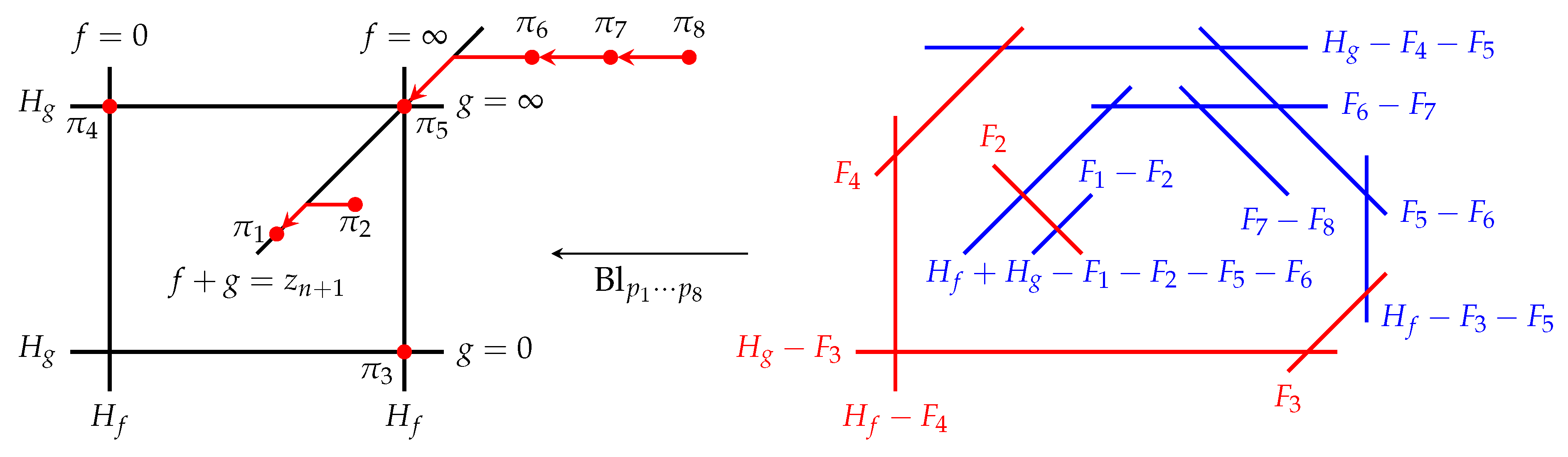
Proof of Theorem 1 (normalizer theory). When
W is an affine Weyl group with a simple system
and a root system
, a subset
defines a
standard parabolic subgroup . If
can be written as a product
of standard parabolic subgroups with
, then we call
the
irreducible components of
J. The standard parabolic subgroup
is itself a Coxeter group, and we can consider the associated root system
. When
is finite, the subset
J is called
spherical, and in this case, the irreducible components of
will be finite Weyl groups. The results of [
25] that we will use state that the normalizer
of
in
W is given by
, where
is the setwise stabilizer of
J, and, further, provide a way to obtain a presentation of
in terms of generators and relations.
To outline the Brink–Howlett construction of the presentation of
, we introduce some notations. For a spherical subset
, we let
denote the unique longest element in
with respect to the usual Bruhat ordering on
W. This is the ordering of elements by length
, defined as the minimal length of an expression for
w in terms of simple reflections. When
, we regard
as the identity element. In the Brink–Howlett framework, disjoint subsets
determine a unique element
, which, in the cases relevant to us, has the following simple description. Let
with
be such that
is finite. Let
and denote by
the union of the irreducible components of
L, which have a non-empty intersection with
I. Then,
is spherical and
When
consists of only a single simple root, we write
, and note that when
corresponds to a node of the Dynkin diagram not joined to any of those corresponding to elements of
J, we have
, since
and
.
For an affine Weyl group
W and
, the group presentation of
is obtained in the Brink–Howlett framework using a groupoid constructed as follows: Let
be the set of
W-associates of
J. Then, consider the set
This has the structure of a groupoid with (partial) operation
. This can be represented as a graph whose vertices correspond to elements of
, with vertices
connected by an edge when there exists
such that
. The graph may also have
loops, i.e., edges from a vertex
to itself, when there exists
such that
.
Then, paths in the graph correspond to elements of
, and elements of
correspond to paths beginning and ending at the vertex
J:
Further,
itself has the structure of a Coxeter group (see [
25] for details), which often turns out to be an affine Weyl group or an extension thereof. The above results do not immediately solve our problem of computing and describing
G, but they take care of most of it. Some extra work is required, which firstly comes from the fact that
is not purely an affine Weyl group and secondly from the fact that we want to compute the setwise stabilizer not of some
, but rather of
, where
J is spherical and
is the highest root of
. With the first fact in mind, we begin by noting that we can view
as the extended affine Weyl group
. To do this, take the simple system
of the
root system in
as above and introduce
In particular, from Equations (
25) and (
4), we see that
,
and
. Then,
forms a simple system for a root system of type
, with the Cartan matrix given by
Here,
is the same bilinear form on
as was used for the
root system, but note that for
B-type root systems, the generalized Cartan matrix is not symmetric. The affine Weyl group
![Mathematics 13 01123 i003]()
is realized as linear transformations of
by the actions of simple reflections
The root system here is then
, and
includes reflections
,
, which act on
by
Note that
is a root of the
-system, so
, but that not all roots of the
-system are roots of the
-system, and, in particular, that the simple reflection
acts on
as the automorphism
of the
Dynkin diagram of the
-system. This is why we use notation
to distinguish the reflections associated to elements of
from the reflections
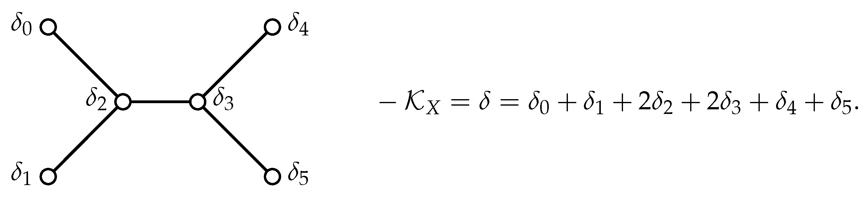
. The single non-trivial automorphism of the
Dynkin diagram is given by
, and we have
, with generators satisfying the defining relations given in Equation (
26), as summarized in
Figure 8:
The generator
of
is not accounted for in this extension, and we have
. The reason for introducing this description is that it makes it easier to apply the normalizer theory to compute the relevant stabilizer—we can now work with an extension of an affine Weyl group by a smaller Dynkin diagram automorphism group. In addition, the different root lengths of the two
root systems in Theorem 1 can be clearly seen in terms of roots of different lengths in the
system.
Note that we can use an element of
, e.g.,
, to send the set
to
, so the group
G we wish to compute is conjugate to
To compute
, we first compute
for
in the affine Weyl group
using the Brink–Howlett method and then find the elements which exchange
and
. Once this has been achieved, finally, we consider the extra elements coming from the extension of
to
.
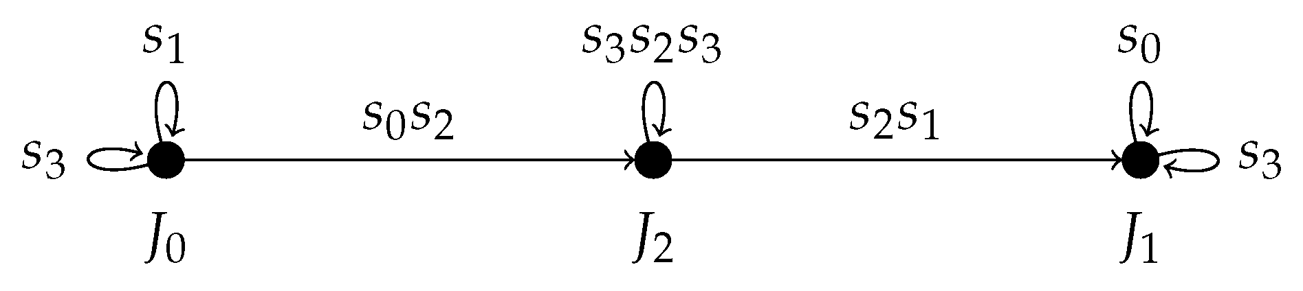
We begin by constructing the graph associated with the groupoid
for
and
. The vertices correspond to
W-associates of
J, the set of which is
where we note that
is not included because
is a short root. To determine where the edges are, one proceeds to calculate, for each vertex
, the element
for each
. If
, then one draws an edge from
to
, labeled by the element
. The graph for the case at hand is given in
Figure 9.
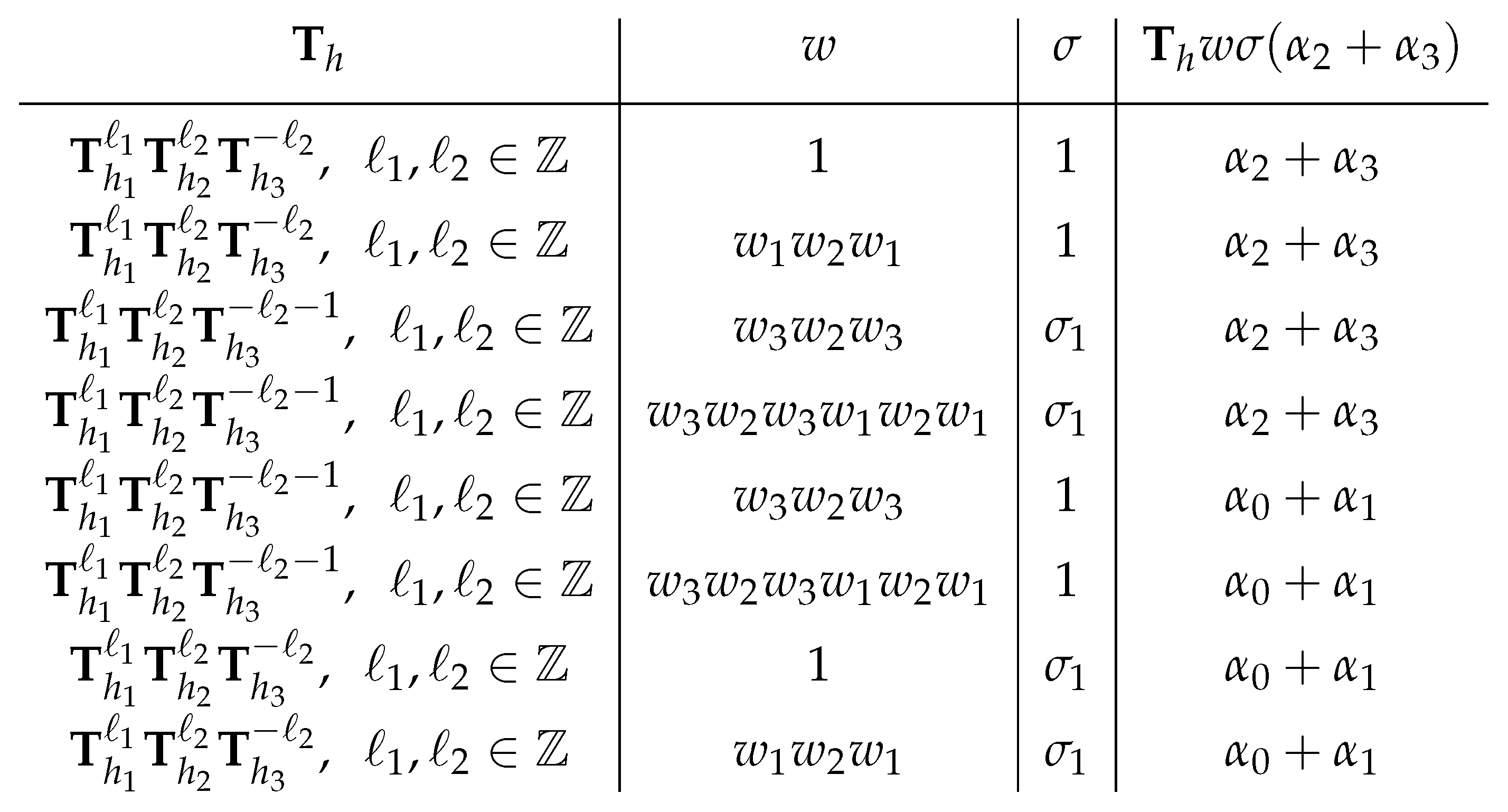
It will be convenient to denote paths in the graph according to the vertices through which they pass read from right to left, e.g., for the path from to . To account for loops, we use the symbol for the element itself, e.g., , to indicate the loop from to itself via . For a path p in this notation, we denote by the composition of the elements corresponding to the edges and loops in the path, e.g., for a path that starts at , traverses a loop via , and then goes to via .
From
Figure 9, we see that the elements
corresponding to paths starting and ending at
can be obtained as compositions of the following elements and their inverses:
where we have identified these as reflections
associated to some roots
.
Invoking the Brink–Howlett result that
consists of elements corresponding to paths starting and ending at
J, we have a set of generators. Since
, we have
Each of the subgroups
,
are individually isomorphic to copies of
defined using simple systems
and
as groups of linear transformations of the subspaces of
spanned by these. We want to describe the quasi-translation elements of
, such as that corresponding to the d-P
II dynamics, as translation elements with respect to the affine Weyl group structure of
. In the case of the non-simply laced type of the ambient group, as we have here with
, this requires some care.
We introduce elements
and
of
to play the roles of simple systems for the two copies
and
of
in
. Since
is a long root of
, we take
, but for the short root
, we instead introduce
, and
. Even though
is not an element of
, by use of the notation, we still write
for the reflection
. This scaling is necessary for the description of quasi-translation elements of
in terms of weights from the affine Weyl group structure of
to be compatible with that of translation elements in terms of the weights of the finite
system, which we will say more about in Remark 1 below. It also demonstrates the origin of the different root lengths of the
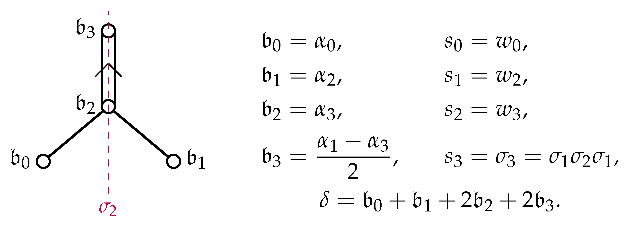
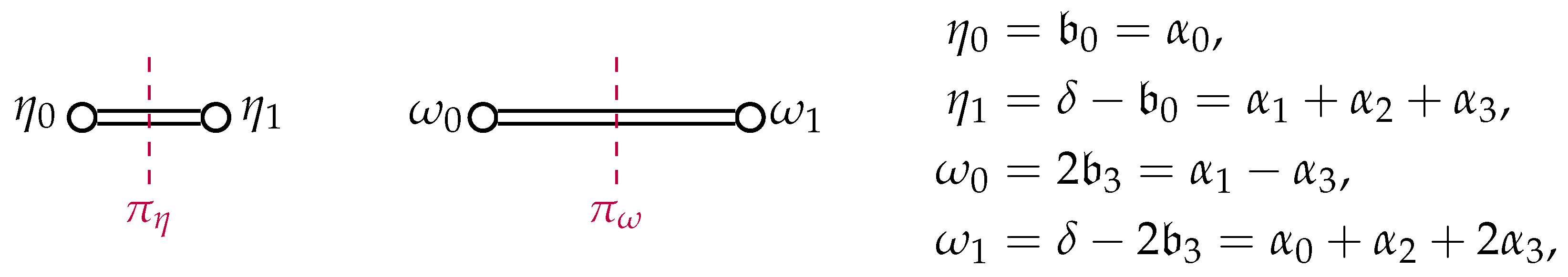
-type systems in Theorem 1. We summarize the
- and
-systems, as well as the relations to the
- and
-systems in
Figure 10.
We next consider the setwise stabilizer in
of not just
but also of
. This is straightforward and we need only to add a single generator since
, where
g is any element such that
. To see this, note that any element of
leaves
invariant, so if
are such that
, then
. We can find such an element immediately as
, which acts on the
as
Adding this element as a generator to the description of
in Equation (
28), we see it causes the addition of a Dynkin diagram automorphism
, as indicated in
Figure 10, since
. We then have
Lastly, we have to consider the elements of
which have not been accounted for as part of
. First, we consider the extension of
to
by adding the generator
, corresponding to the automorphism of the
Dynkin diagram that permutes the simple roots according to
. We see that
does not add any new elements to the stabilizer beyond
already found, since
. Finally, considering the extra Dynkin diagram automorphism
which is not accounted for in
, we see that this does indeed add a new generator to the stabilizer. We have
, and
, so because
is an involution, we have
. To determine whether this extension adds any elements to the setwise stabilizer of
, we just have to determine whether there exist
such that
. In this case, we would obtain a new element
such that
. This does indeed happen. For example,
with
, and we obtain an element corresponding to the remaining automorphism of the
diagram
. Note that adding
as a generator to
accounts for all of the set
. This is because if
,
, with
, are such that
, then
, and also
already includes all elements of
that interchange
and
.
We then arrive at the desired description of the setwise stabilizer
where expressions for the generators in terms of those of
and
are collected below:
Finally, we conjugate the generators of
by
to obtain the description of
G in Theorem 1 via
and we are done. □


 can now be realized via reflections in the roots , , which can be defined on the whole of ,
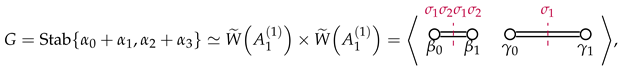 where
where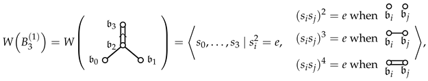 is realized as linear transformations of by the actions of simple reflections The root system here is then , and includes reflections , , which act on by