Enhancing Neural Network Training Through Neuroevolutionary Models: A Hybrid Approach to Classification Optimization

Abstract

The optimization of Artificial Neural Networks (ANNs) remains a significant challenge in machine learning, particularly in overcoming local-optima limitations during training. Traditional classification algorithms, such as k-Nearest Neighbors (KNN), decision trees, Support Vector Machines (SVMs), and ANNs, often suffer from convergence to suboptimal solutions due to their training methods. This research proposes a hybrid neuroevolutionary approach that integrates a genetic algorithm with a NEAT-based structure to enhance ANN performance. Additionally, a Cellular Processing Algorithm (PCELL) is employed to expand the search space and improve solution quality. The methodology involves designing an initial neural network trained via backpropagation, followed by the application of genetic operators to evolve network structures. Experimental results from diverse benchmark datasets demonstrate that the proposed algorithm outperforms conventional ANN training methods and achieves performance levels comparable to evolutive solutions. The results suggest that integrating evolutionary strategies with cellular processing enhances classification accuracy and contributes to the advancement of neuroevolutionary learning techniques.

1. Introduction

Machine learning is widely used to address complex classification problems across diverse research domains [1,2,3]. Among its techniques, Artificial Neural Networks (ANNs) stand out due to their adaptability and ability to model intricate patterns [4]. However, conventional ANN training methods, such as backpropagation, often struggle with hyperparameter optimization and the risk of becoming trapped in local optima, limiting their generalization ability. Additionally, configuring ANN architectures requires extensive experimentation, making the training process computationally expensive and time-consuming [5]; to overcome these challenges, researchers have explored diverse optimization strategies, with evolutionary algorithms emerging as a promising approach [6,7]. These methods, inspired by biological evolution, effectively search for optimal solutions to high-complexity problems. Specifically, combining ANNs with evolutionary algorithms has led to neuroevolutionary networks, which integrate genetic evolution mechanisms into the training phase to enhance performance and avoid suboptimal convergence [8,9].

Artificial Neural Networks (ANNs) have been widely applied in diverse domains, including image recognition [10], natural language processing [11], and medical diagnosis [12], among others. The ability of ANNs to model complex patterns makes them essential tools in machine learning. However, traditional training methods for ANNs often face challenges with local optima, which limits the network’s ability to achieve a better solution. The complexity of hyperparameter tuning further exacerbates this issue, requiring extensive experimentation to find configurations that enhance performance [13].

Evolutionary algorithms (EAs) offer an alternative approach to optimizing neural networks by mimicking biological evolution through selection, mutation, and crossover operators. Neuroevolution, which integrates EAs into ANN training, optimizes neural networks by evolving a population of candidate models through genetic operators. Each iteration generates a new population where networks gradually adapt their architectures and weights based on their performance, enabling a form of evolutionary learning. This approach has demonstrated improvements in network adaptability and convergence [14,15], as neural networks function as adaptive agents that refine their structure and parameters over time to enhance performance in a given task.

Unlike conventional methods that require predefined architectures, the NeuroEvolution of Augmenting Topologies (NEAT) allows networks to grow in complexity by introducing new neurons and connections during the training phase. Additionally, NEAT employs reinforcement mechanisms to guide the evolutionary process, enabling unsupervised learning and fostering structural innovation within evolving populations [16]. Several variants of NEAT, such as HyperNEAT [17], Hybrid Self-Attention NEAT [18], and CoDeepNEAT [19], have been proposed to enhance the efficiency and scalability of neuroevolution. However, these approaches typically involve higher computational costs and increased complexity due to the need for more sophisticated search strategies and larger solution spaces. In this work, we focus on the base NEAT approach to maintain a balance between computational efficiency and model complexity. In [20], Li et al. proposed a novel Recurrent NEAT-based MUSIC (RNEAT-MUSIC) algorithm to optimize 2D-DOA estimation by reducing computational complexity without compromising accuracy. Their approach leverages the NEAT framework, which evolves neural network architectures dynamically, allowing for adaptive learning without requiring predefined structures. To further enhance efficiency, the proposed model incorporates a recurrent structure within NEAT, minimizing the number of required neural network parameters and reducing the overall computational burden. The algorithm extracts phase components from the received signal covariance matrix, applying a reduced-dimensional neural network to restrict the scanning region before executing the computationally expensive MUSIC stage. Experimental validation demonstrates that RNEAT-MUSIC achieves a 75% reduction in computational workload compared to traditional 2D-MUSIC while preserving high-resolution DOA estimation. The results indicate that this approach effectively balances exploration and exploitation in neuroevolutionary learning, improving adaptability and convergence speed. These findings position RNEAT-MUSIC as a promising alternative for real-time satellite tracking, offering a computationally efficient solution for high-precision DOA estimation in space communication applications.

Despite NEAT advantages, maintaining an effective balance between exploration and exploitation remains challenging, as genetic algorithms risk premature convergence or high computational costs when optimizing complex network structures. To address these limitations, this study proposes a hybrid neuroevolutionary approach that integrates Cellular Processing Algorithms (PCELL) with NEAT-based networks. PCELL is inspired by cellular automata, where a system is divided into discrete units (cells) that evolve based on local interactions and predefined rules [21]. This decentralized processing enhances computational efficiency and facilitates parallel optimization, making it particularly useful for evolving complex neural architectures. By structuring the solution space into smaller, interacting regions, PCELL mitigates premature convergence and fosters greater diversity in evolutionary processes [22]. Integrating PCELL with NEAT expands the solution search space, refines network topologies, and improves classification accuracy by promoting structural adaptation throughout the evolutionary process.

In this paper, we propose optimizing neural network training using neuroevolutionary models. It proposes developing a Cellular Processing Algorithm to control the evolution of these networks, improving hyperparameter tuning and learning efficiency. The experimental phase involves training and evaluating the proposed model on benchmark datasets to assess its effectiveness against state-of-the-art classification techniques.

This research contributes to the field of machine learning by developing novel genetic operators for neural networks, introducing a hybrid methodology that optimizes the training process and delivers superior classification results. The study builds on advanced optimization techniques and validates the proposed models experimentally to provide more robust and efficient solutions in artificial intelligence.

The remainder of this paper is organized as follows: Section 2 presents the materials and methods; Section 3 describe the experimentation results and the discussion; and, finally, Section 4 presents the conclusions and future work.

2. Materials and Methods

To assess the algorithm robustness, for this work, we consider a set of independent instances with varying characteristics, such as the number of registers and dataset dimensionality. The selection criterion included datasets for classification with at least two evaluation classes and no missing values. The chosen datasets were obtained from publicly available machine learning repositories, specifically Kaggle [23] and the UCI Machine Learning Repository [24], providing diverse and well-structured data for a comprehensive performance analysis.

Table 1. Characteristics of the selected datasets for experimentation.

Dataset Name	Repository	Data Type	Registers	Attributes	Classes
banknote_auth	UCI	Integer/Real	1372	4	2
divorce	UCI	Integer/Real	170	54	2
iris	Kaggle	Integer/Real	150	4	3
pulsar_stars	Kaggle	Integer/Real	17,898	8	2
car_evaluation	UCI	Categorical	1728	6	4
contact-lenses	UCI	Categorical	24	4	3
weather.nominal	UCI	Categorical	14	4	2
diabetes	Kaggle	Integer/Real	768	8	2
weather.numeric	UCI	Categorical	14	4	2
QSAR Bioconcentration	Kaggle	Integer/Real	779	9	3
seeds	UCI	Integer/Real	210	7	3
cryotherapy	UCI	Integer/Real	90	6	2
Heart_disease	Kaggle	Integer/Real	303	13	2
glass	Kaggle	Integer/Real	214	9	7
abalone	UCI	Categorical	4177	8	29

shows the characteristics of each selected dataset, where columns show the name of the dataset, the repository from which the dataset was extracted, the data types of the corresponding attributes of each dataset, and the number of registers, attributes, and classes.

2.1. Preprocessing

Once the instances were defined, we applied a normalization method. For this work, we decided on the normalization method to be used to transform each dataset. We used a normalization; this process rescales data to a specific range, typically between 0 and 1 or −1 and 1, ensuring a consistent scale across feature. Moreover, standardization adjusts data by centering them around a mean of 0 and scaling them to have a standard deviation of 1. This technique preserves the original distribution and is particularly effective when working with normally distributed data.

For the selection of the normalization method, each attribute of each dataset was reviewed to evaluate which type of standardization would be applied, considering if the attributes presented a normal distribution after we applied standardization, and, in cases where the data needed rescaling, we applied normalization.

Table 2. Attribute information sample for preprocessing.

Attribute	Min	Max	Mean	Standar Deviation	Decision
banknote_auth
a1	−7.0421	6.8248	0.43373526	2.84172641	Std
a2	−13.7731	12.9516	1.92235312	5.86690749	Norm
a3	−5.2861	17.9274	1.39762712	4.30845909	Std
a4	−8.5482	2.4495	1.19165652	2.10024732	Std
Iris
a1	4.3	7.9	5.84333333	0.82530129	Norm
a2	2	4.4	3.054	0.43214658	Norm
a3	1	6.9	3.75866667	1.75852918	Norm
a4	0.1	2.5	1.19866667	0.76061262	Norm
pulsar_stars
a1	5.8125	192.617188	111.079968	25.6522187	Std
a2	24.7720418	98.7789107	46.5495316	6.84299824	Std
a3	−1.87601118	8.06952205	0.47785726	1.06400999	Std
a4	−1.79188598	68.1016217	1.770279	6.16774094	Std
a5	0.2132107	223.392141	12.6143997	29.4720738	Std
a6	7.37043217	110.642211	26.3265147	19.4700284	Std
a7	−3.13926961	34.5398442	8.30355612	4.50596597	Std
a8	−1.9769756	1191.00084	104.857709	106.511564	Std
Heart_disease
a1	29	77	54.3663366	9.06710164	Norm
a2	0	1	0.68316832	0.46524119	-
a3	0	3	0.9669967	1.03034803	Norm
a4	94	200	131.623762	17.5091781	Std
a5	126	564	246.264026	51.745151	Std
a6	0	1	0.14851485	0.3556096	-
a7	0	2	0.52805281	0.52499112	Std
a8	71	202	149.646865	22.8673326	Std
a9	0	1	0.32673267	0.46901859	-
a10	0	6.2	1.03960396	1.15915747	Std
a11	0	2	1.39933993	0.61520843	Std
a12	0	4	0.72937294	1.0209175	Std
a13	0	3	2.31353135	0.61126531	Std
Abalone
a1	1	3	2.04452957	0.8277156	-
a2	15	163	104.79842	24.0157072	Std
a3	11	130	81.5762509	19.8455972	Std
a4	0	226	27.9032799	8.3644099	Std
a5	0.4	565.1	165.748432	98.0660627	Std
a6	0.2	297.6	71.8734977	44.3872756	Std
a7	0.1	152	36.1187216	21.9202257	Std
a8	0.3	201	47.7661719	27.8372011	Std

shows a sample of the results of the analysis performed for the selection of the normalization technique for all datasets, where columns show the attribute number of the dataset, the statistical information for each attribute (minimum value, maximum value, mean, and standard deviation), and the decision taken to normalize each attribute, where the norm is obtained from Equation (1), std is calculated with Equation (2), and the − symbol indicates that no normalization method was required for this attribute.

$$Norm\left(x_i\right)={\displaystyle \frac{x_i-mi{n}_{val}}{ma{x}_{val}-mi{n}_{val}}}$$

(1)

$$Std\left(x_i\right)={\displaystyle \frac{x_i-\overline{x}}{\sigma }}$$

(2)

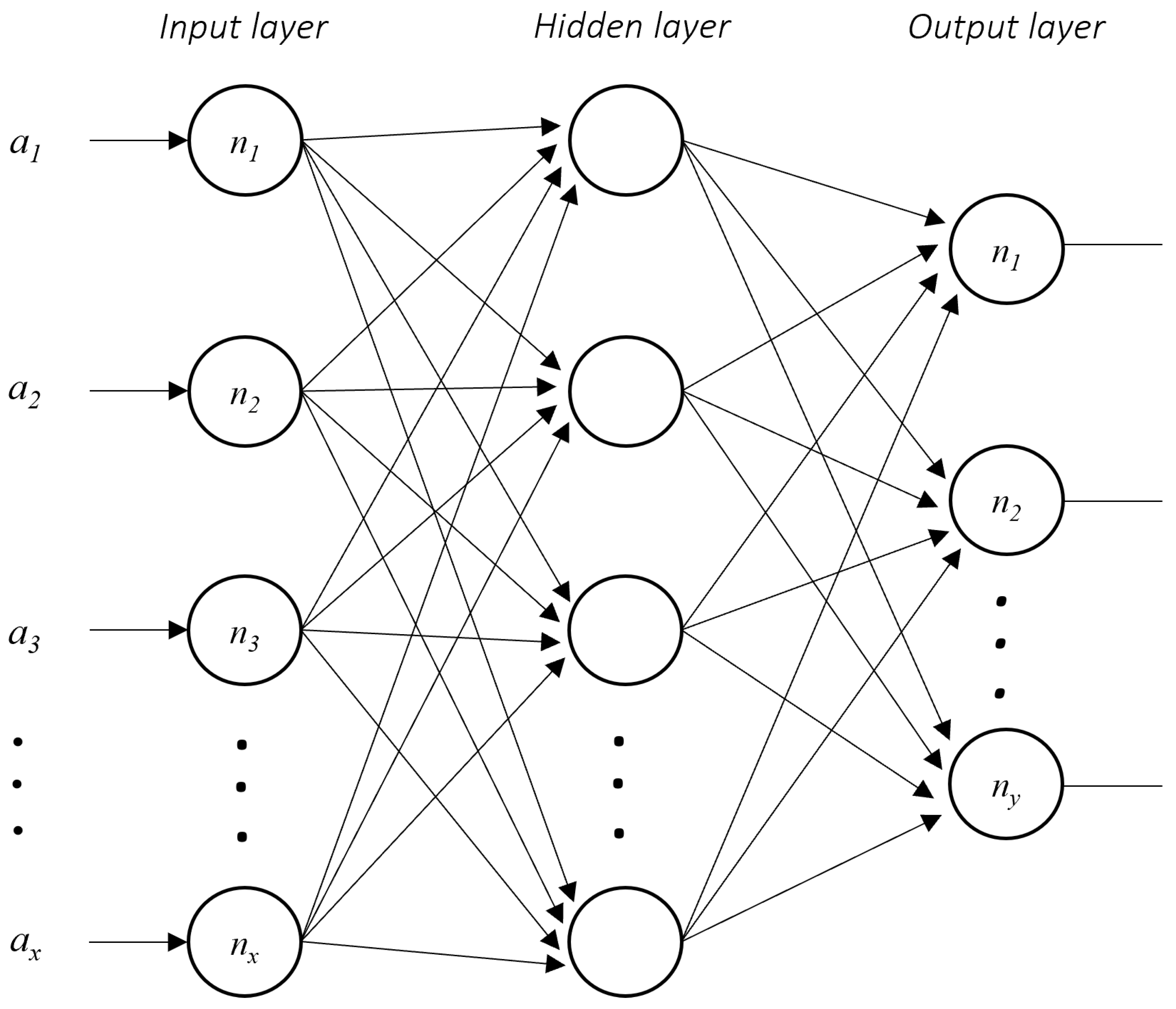
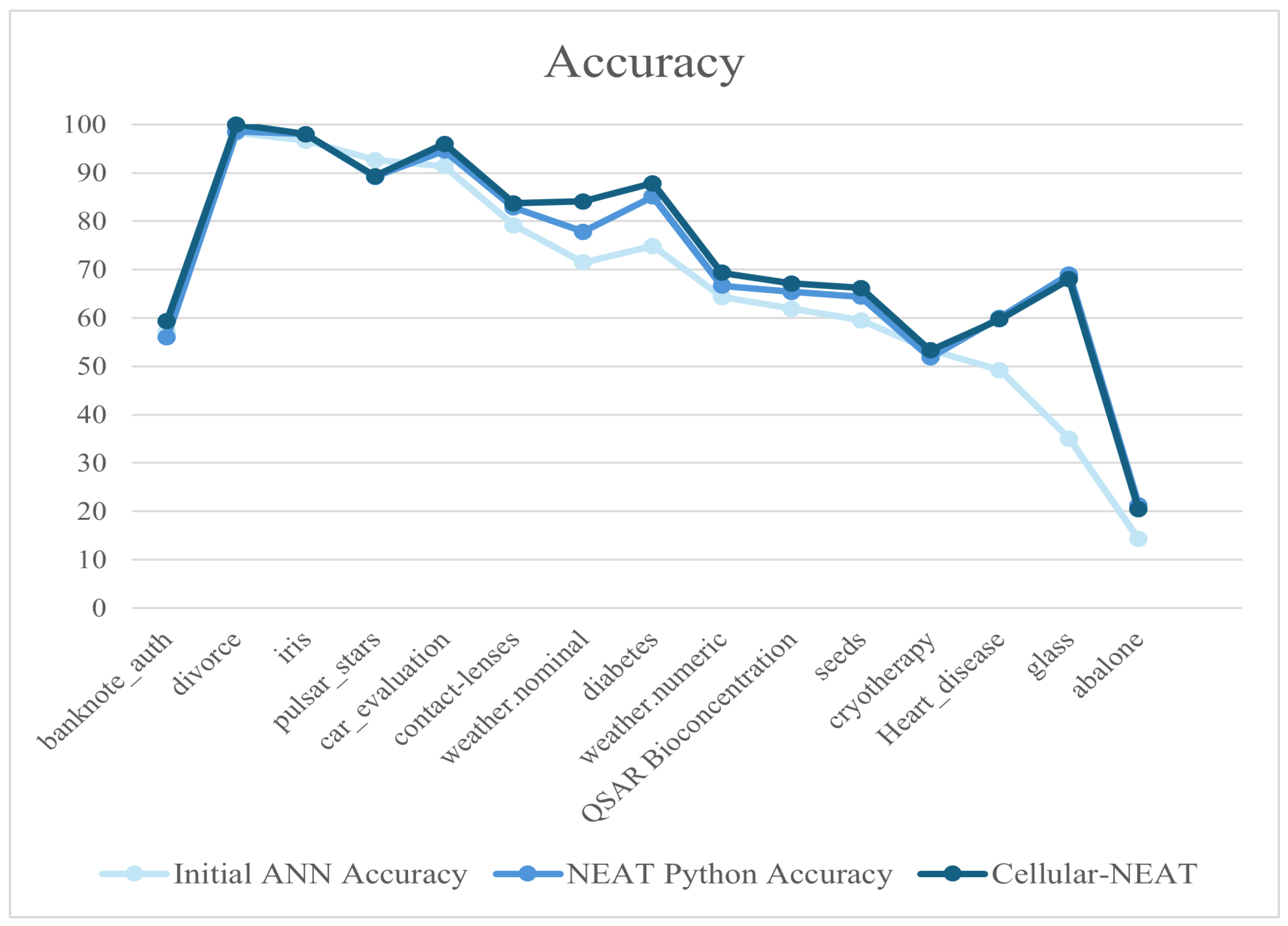
In addition, we perform an Artificial Neural Network with the TensorFlow library in Python to have an accuracy reference value. The Artificial Neural Network structure for this experiment was an input layer with the number of neurons equal to the number of attributes, a hidden layer with the same number of neurons as the input layer, and an output layer with one neuron. Each dataset was divided into training and testing. The production percentages of each set in the experimentation were 70% training and 30% test.

2.2. NEAT Algorithm

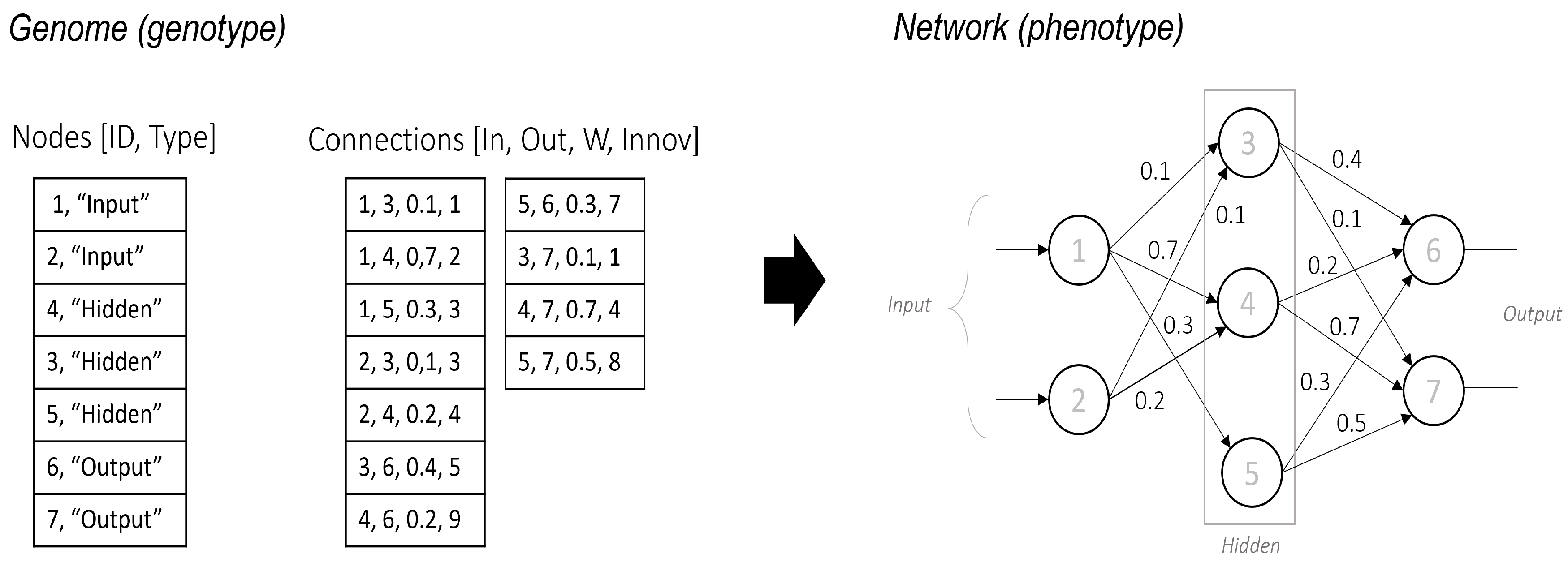
For the neuroevolution of neural networks, we apply the NeuroEvolution of Augmenting Topologies (NEAT) algorithm [25], which evolves Artificial Neural Networks through mutation and selection. The genetic coding scheme represents the neural network in two phases: genotype and phenotype.

To encode the genome, NEAT utilizes a list of nodes and a list of connections. The Nodes list defines neurons within the network, each uniquely identified by an $ID$ and categorized as input, hidden, or output. The Connections list specifies synaptic links between neurons, encoding key attributes such as input and output nodes, connection weight w, and innovation number $innov$, which ensures the historical tracking of mutations.

Figure 1 also shows the phenotype, where the neural network structure emerges from the encoded genome. Input neurons receive data, hidden neurons process information, and output neurons generate final predictions. The structural complexity of the network increases as mutations introduce new nodes and connections, enabling adaptive evolution.

This encoding strategy ensures a direct mapping between genotype and phenotype, supporting both structural and parametric evolution while preserving innovation through historical markings. As a result, NEAT effectively optimizes neural network architectures by balancing the exploration of new topologies and the inheritance of beneficial traits.

2.3. Evolution Process

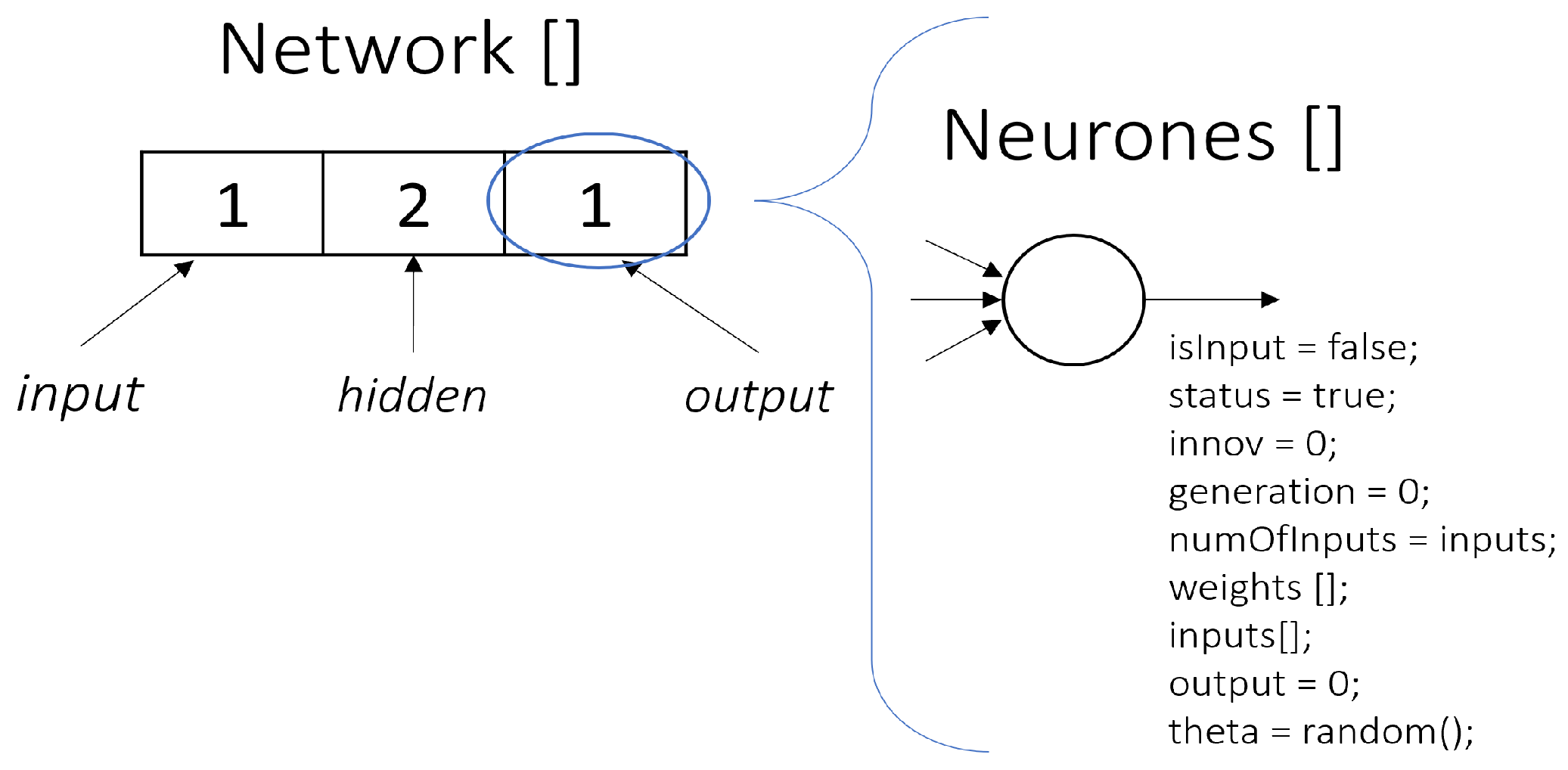
In this paper, we propose a modified genetic encoding scheme for a neural network within the NeuroEvolution of Augmenting Topologies (NEAT) algorithm. This adaptation incorporates structural modifications to the genotype by integrating additional connection parameters and representing the phenotype as a structured list format as shown in Figure 2.

At the genotypic level, the encoding includes a set of connection attributes, specifying details such as activation states (e.g., true/false flags), numerical weights (float values), and additional properties that refine the mutation and selection mechanisms. These modifications enhance the expressiveness of the genome, allowing for greater control over the evolutionary process.

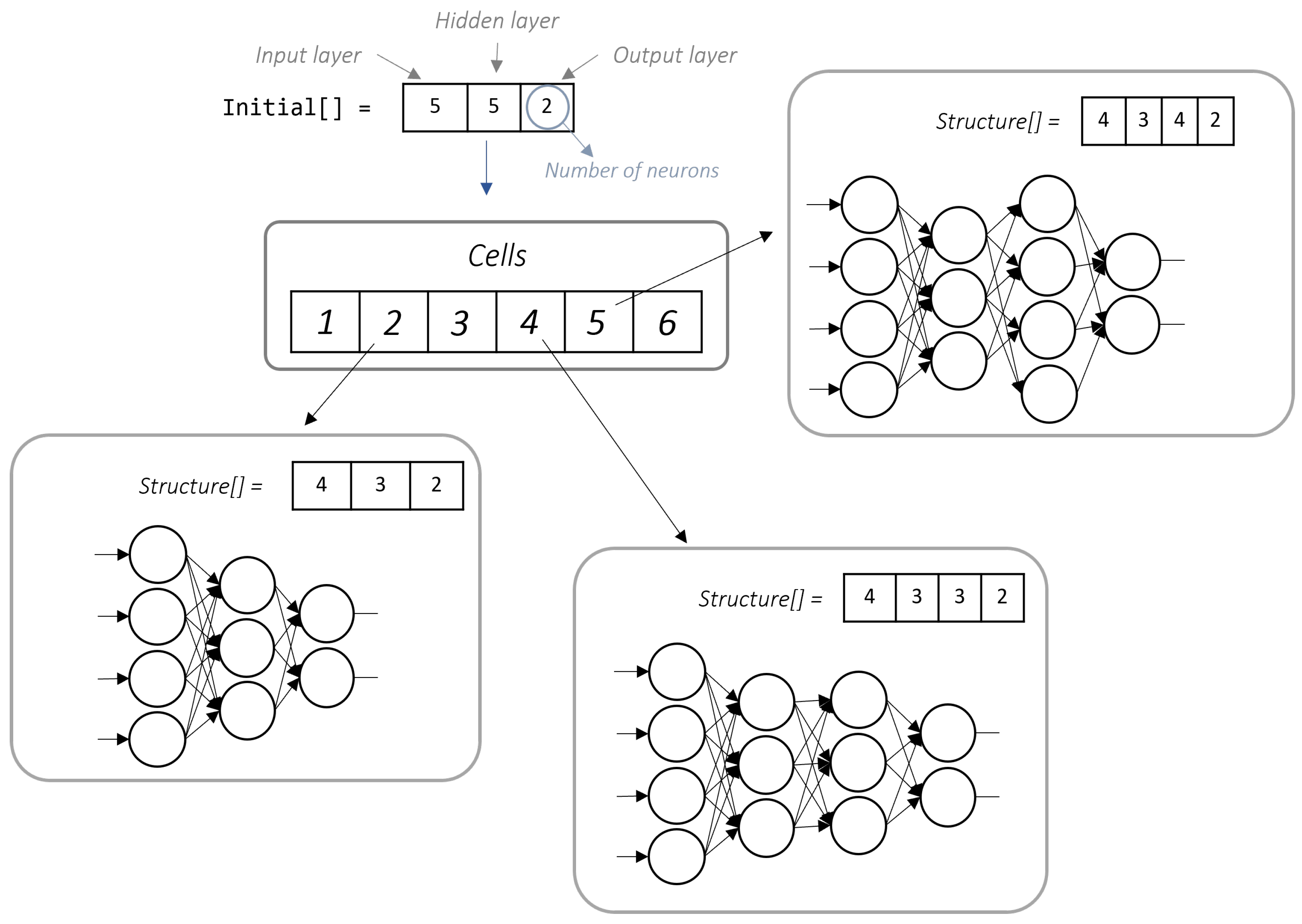
The phenotype is represented as a list (network), where the first element corresponds to the number of neurons in the input layer, followed by elements representing the number of neurons in each hidden layer. The final element in the list denotes the number of neurons in the output layer. This structured format provides an intuitive representation of the neural network architecture, enabling the efficient manipulation and analysis of evolving topologies.

The proposed genome was used in conjunction with a genetic algorithm to develop a genetic algorithm aimed at enhancing neural network development.

Genetic algorithms (GAs) [26] are optimization techniques inspired by the principles of natural selection and genetics. GAs operate by evolving a population of candidate solutions through iterative processes of selection, crossover, and mutation, aiming to find optimal or near-optimal solutions to complex problems. In the context of neural networks, GAs have been employed to optimize various aspects, including network architecture [27,28], weights [29,30], and hyperparameters [31,32].

The genome structures of the neural network were developed for the initial population of the genetic algorithm. The algorithm began by selecting candidates for the generation through a binary tournament.

For genetic operators, mutation and crossover methods were designed based on the NEAT genome. The mutation method introduced changes at the genotype level, specifically modifying the weight on a specific connection. Algorithm 1 modifies the structure of neural networks by adjusting the weights and innovation numbers within the hidden layers. The procedure begins by selecting a random hidden layer and a neuron within that layer. A specific weight from the selected neuron is then chosen and modified. Then, the algorithm increments the innovation numbers for the hidden layer and the neuron to reflect the changes and updates the chosen weight with a new random value.

Algorithm 1 Genoytpe Mutation Operator

1: procedure $GenOperator$($NeuralNetwork$$Of fsprings\left[\right]$)  2:       for each $\mathrm{i}\mathbf{in}\mathrm{Offs}$ do  3:        $HL=$ $rand$(0, $(Of fs[i].hidL)-1$)  4:        $N=$ $rand$(0, $(Of fs[i].hidL[HL].neurons)-1$)  5:        $w_m=$ $rand$(0, $(Of fs[i].hidL[HL].neurons[N].w)-1$)  6:        $Of fs\left[i\right].hidL\left[HL\right].innov=Of fs\left[i\right].hidL\left[HL\right].innov+1$  7:        $Of fs\left[i\right].hidL\left[HL\right].neurons\left[N\right].innov=Of fs\left[i\right].hidL\left[HL\right].neurons\left[N\right].innov+1$  8:        $Of fs\left[i\right].hidL\left[HL\right].neurons\left[N\right].w=Of fs\left[i\right].hidL\left[HL\right].neurons\left[N\right].w\left[w_m\right]$  9:        $Of fs\left[i\right].hidL\left[HL\right].neurons\left[N\right].w\left[w_m\right]=$$rand\left(\right)$ 10:       end for 11: end procedure

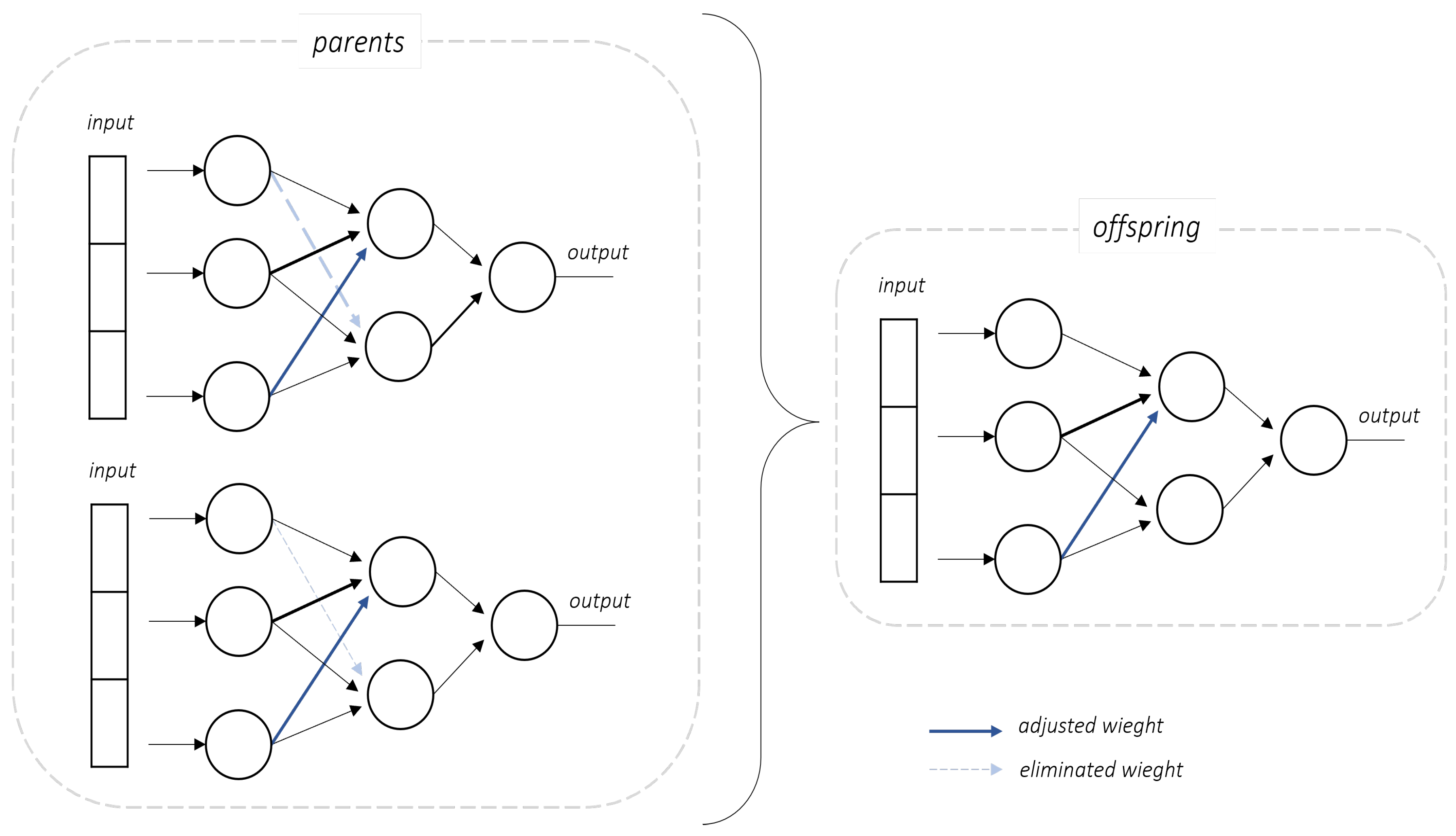
For crossover, modifications were applied to the genome’s information regarding the connections within the neural network. The crossover operator consists of a differential evolution strategy within a neural network framework. It adjusts the network weights based on differences computed from two-parent networks and introduces stochastic mutations while tracking modifications via innovation counters, as illustrated in Figure 3.

Algorithm 2 modifies the neural network structure based on evolutionary principles. It processes three neural networks, denoted as $p_1$, $p_2$, and $p_3$, along with an integer parameter numEdges, which represents the total number of edges in the network.

Algorithm 2 Differential Crossover Operator

1: procedure gendc_operator($p1,p2,p3,numEdges$)  2:     $mods=\lfloor numEdges\times 0.05\rfloor$  3:     for $j=0$ to $mods-1$ do  4:          $HL=\mathrm{rand}(0,\mathrm{length}(p1\left[0\right].hidL)-1)$  5:          $N=\mathrm{rand}(0,\mathrm{length}(p1\left[0\right].hidL\left[HL\right].neurons)-1)$  6:          $w_m=\mathrm{rand}(0,\mathrm{length}(p1\left[0\right].hidL\left[HL\right].neurons\left[N\right].weights)-1)$  7:          $w_{p1}=p1\left[0\right].hidL\left[HL\right].neurons\left[N\right].weights\left[w_m\right]$  8:          $w_{p2}=p2\left[0\right].hidL\left[HL\right].neurons\left[N\right].weights\left[w_m\right]$  9:          $w_{Temp}=(w_{p1}-w_{p2})\times v$ 10:          $p=\mathrm{rand}(0,1)$ 11:          if $p \le fathe{r}_{probability}$ then 12:          $w_{mod}=p3.hidL\left[HL\right].neurons\left[N\right].weights\left[w_m\right]$ 13:          $w_{Temp}=w_{Temp}+w_{mod}$ 14:          $p3.hidL\left[HL\right].innov=p3.hidL\left[HL\right].innov+1$ 15:          $p3.hidL\left[HL\right].neurons\left[N\right].innov=p3.hidL\left[HL\right].neurons\left[N\right].innov+1$ 16:          $p3.hidL\left[HL\right].neurons\left[N\right].lastW=w_{mod}$ 17:          $p3.hidL\left[HL\right].neurons\left[N\right].weights\left[w_m\right]=w_{Temp}$ 18:          else 19:          $p3.hidL\left[HL\right].innov=p3.hidL\left[HL\right].innov+1$ 20:          $p3.hidL\left[HL\right].neurons\left[N\right].innov=p3.hidL\left[HL\right].neurons\left[N\right].innov+1$ 21:          $p3.hidL\left[HL\right].neurons\left[N\right].lastW=p3.hidL\left[HL\right].neurons\left[N\right].weights\left[w_m\right]$ 22:          $p3.hidL\left[HL\right].neurons\left[N\right].weights\left[w_m\right]=w_{Temp}$ 23:          end if 24:     end for 25:     return $p3$ 26: end procedure

The number of modifications applied is computed as

$$\mathrm{mods}=\lfloor \mathrm{numEdges}\times 0.05\rfloor$$

(3)

The algorithm iterates for $j=0,1,\dots ,\mathrm{mods}-1$, and, in each iteration, it performs the following steps. A hidden layer index HL is selected randomly, followed by a neuron index N within that layer and a weight index $w_m$ from the neuron’s weight vector. These indices define a specific weight to modify. The corresponding weights from $p_1$ and $p_2$ are retrieved:

$$w_{p1}=p_1.\mathrm{hidL}\left[HL\right].\mathrm{neurons}\left[N\right].\mathrm{weights}\left[w_m\right]$$

(4)

$$w_{p2}=p_2.\mathrm{hidL}\left[HL\right].\mathrm{neurons}\left[N\right].\mathrm{weights}\left[w_m\right]$$

(5)

The new weight is computed as

$$w_{\mathrm{Temp}}=(w_{p1}-w_{p2})·v$$

(6)

where v is a predefined scalar multiplier defined by experimentation.

A probability value p is sampled from a uniform distribution in $[0,1]$. If $p \le fathe{r}_{probability}$, which consists of the probability of selecting a third parent as a candidate to improve the solution as determined using Grid Search, where the final value selected was 0.30, a crossover occurs by incorporating a weight modification from $p_3$:

$$w_{\mathrm{mod}}=p_3.\mathrm{hidL}\left[HL\right].\mathrm{neurons}\left[N\right].\mathrm{weights}\left[w_m\right]$$

(7)

The temporary weight is then updated:

$$w_{\mathrm{Temp}}=w_{\mathrm{Temp}}+w_{\mathrm{mod}}$$

(8)

In both cases, the algorithm updates the innovation counters:

$$p_3.\mathrm{hidL}\left[HL\right].\mathrm{innov}=p_3.\mathrm{hidL}\left[HL\right].\mathrm{innov}+1$$

(9)

$$p_3.\mathrm{hidL}\left[HL\right].\mathrm{neurons}\left[N\right].\mathrm{innov}=p_3.\mathrm{hidL}\left[HL\right].\mathrm{neurons}\left[N\right].\mathrm{innov}+1$$

(10)

The last stored weight is also updated accordingly:

$$p_3.\mathrm{hidL}\left[HL\right].\mathrm{neurons}\left[N\right].w_m=p_3.\mathrm{hidL}\left[HL\right].\mathrm{neurons}\left[N\right].\mathrm{weights}\left[w_m\right]$$

(11)

Finally, the modified weight is assigned:

$$p_3.\mathrm{hidL}\left[HL\right].\mathrm{neurons}\left[N\right].\mathrm{weights}\left[w_m\right]=w_{\mathrm{Temp}}$$

(12)

Once the offspring are generated, the neural network’s accuracy serves as the objective function for the next phase.

The genetic algorithm (GA) used follows a structured approach to optimizing neural network configurations. An individual represents a neural network genotype, and each candidate solution consists of a structured list defining the number of neurons in each layer and their associated connection weights.

The binary tournament technique was used as a selection operator, ensuring diversity while prioritizing high-performing individuals [33]. For example, given two candidates A and B with fitness scores $f\left(A\right)=0.85$ and $f\left(B\right)=0.78$, the selection of the best individual is as follows:

$$S=argmax\left(f\right(A),f(B\left)\right)=A$$

We applied the differential evolution strategy for crossover, where weight adjustments are computed based on differences between two parent networks. If two-parent weights are $w_1=0.5$ and $w_2=0.3$ with a scaling factor $v=0.7$, the new weight is computed as

$$w_{\mathrm{new}}=w_1+v·(w_2-w_1)=0.5+0.7·(0.3-0.5)=0.36$$

With a probability of 0.3, an additional modification is introduced using a third parent’s weight $w_3=0.6$:

$$w_{\mathrm{final}}=w_{\mathrm{new}}+0.3·(w_3-w_{\mathrm{new}})=0.36+0.3·(0.6-0.36)=0.43$$

The mutation process occurs by introducing weight perturbations in randomly selected connections. For example, if we consider a mutation rate of 0.1 to a weight $w=0.43$, the mutation modifies it as

$$w^{\prime }=w+\mathcal{N}(0,{\sigma }^2),\mathrm{where}\sigma =0.05$$

Thus, if $\mathcal{N}(0,0.{05}^2)$ generates a value of 0.02, the new weight is

$$w^{\prime }=0.43+0.02=0.45$$

The replacement technique adopts an elitist strategy, preserving the best solutions across generations to maintain stable convergence. If the best solution in generation t has $f_{max}=0.92$ and in generation $t+1$ a candidate achieves $f=0.95$, the elite strategy ensures retaining the new best solution.

The GA parameters, mutation, and crossover probability were tuned through Grid Search, ensuring an optimal balance between maintaining diversity and refining promising network architectures.

2.4. Cellular Processing

To enhance the quality of the solution obtained by the genetic algorithm, the search space was expanded using a Cellular Processing Algorithm (PCELL). This model simulates the communication and information-processing mechanisms of biological cells.

In this work, PCELL utilized six processing cells, each containing a distinct neural network phenotype derived from the initial solution. Additionally, each cell incorporated the proposed genetic algorithm to explore local solutions effectively.

Algorithm 3 begins by initializing an initial solution $S_0$, which serves as the basis for generating a set of N processing cells $\mathcal{C}=\{C_1,C_2,\dots ,C_N\}$. Each cell $C_i$ is assigned a unique phenotype ${\varphi }_i$ based on a transformation function applied to $S_0$, given by ${\varphi }_i=f(S_0,{\theta }_i)$, where ${\theta }_i$ represents a diversity parameter to explore different regions in the search space. Within each processing cell, a GA iteratively optimizes the assigned solution, leading to an update step defined as $S_i^{(t+1)}=GA\left(S_i^{\left(t\right)}\right)$. The best solution found in each cell is evaluated and stored as $x^{*}$ (Equation (13)), where $f\left(x\right)$ is the objective function to maximize.

$$x^{*}=arg\underset{x\in \mathcal{S}}{max}f\left(x\right)$$

(13)

After processing all cells, the global best solution $x_{global}^{*}$ updates according to

$$x_{global}^{*}=max\{x_{global}^{*},x_{C_i}^{*}\},\forall i\in \{1,...,6\}.$$

(14)

This process continues iteratively until a stopping criterion is met, which is defined when a predefined number of iterations is reached or when the improvement in $x_{global}^{*}$ global falls below a threshold $\epsilon$. Finally, the algorithm returns the most-optimized solution obtained.

Algorithm 3 Cellular Processing

1: Input: Initial solution $S_0$, number of cells N 2: Generate N processing cells $\mathcal{C}=\{C_1,C_2,\dots ,C_N\}$ 3: for each cell $C_i$ do 4:     ${\varphi }_i=f(S_0,{\theta }_i)$ 5:     $S_i^{(t+1)}=GA\left(S_i^{\left(t\right)}\right)$ 6:     $x_{C_i}^{*}=arg{max}_{x\in C_i}f\left(x\right)$ 7: end for 8: $x_{global}^{*}=max\{x_{global}^{*},x_{C_i}^{*}\}$ 9: Output: $x_{global}^{*}$

Algorithm Complexity

The PCELL algorithm divides the search into N independent cells, where N is the number of cells, G represents the number of generations per cell, P denotes the population size in each cell, C stands for the cost of applying genetic operators (mutation, crossover, etc.) to a candidate, and E indicates the cost of evaluating the objective function for each candidate; in this case, the overall temporal complexity is expressed as

$$T_{\mathrm{PCELL}}=O\left(N·G·P·(C+E)\right)$$

(15)

A conventional genetic algorithm that operates on a single population has a temporal complexity of

$$T_{\mathrm{GA}}=O\left(G·P·(C+E)\right)$$

(16)

Comparing Equations (15) and (16) shows that the computational cost of the PCELL approach increases by a factor of N. Although this factor raises the computational load, the parallel exploration of multiple cells enhances the diversity in the search for solutions.

In backpropagation, the training process iterates over the dataset to update the network parameters, where I represents the number of iterations (epochs) and M denotes the total number of parameters (weights and biases) in the network; accordingly, the complexity approximates to

$$T_{\mathrm{BP}}=O\left(I·M\right)$$

(17)

Equation (17) indicates a lower cost per iteration compared to Equation (15); this method risks becoming trapped in local optima and does not explore the solution space as efficiently.

The PCELL approach exhibits a temporal complexity of $O\left(N·G·P·(C+E)\right)$, which exceeds that of a traditional ($O\left(G·P·(C+E)\right)$) due to the factor N. This extra cost justifies itself by the improvement in the exploration of the solution space. Additionally, the backpropagation method has a complexity of $O\left(I·M\right)$, which generally offers higher efficiency per iteration but may not provide the global search robustness achieved by evolutionary methods.

This comparison clarifies the implications of the increased computational cost of the PCELL approach compared to traditional methods and highlights the trade-off between computational efficiency and the ability to explore diverse solutions.

3. Results and Discussion

For the development of this work, we used an HP ENVY Laptop 13-ad0xx, equipped with an Intel Core i7-7500U CPU @ 2.70GHz (2.094 GHz), 8 GB DDR3 SDRAM, and running Microsoft Windows 10 Home Single Language, version 10.0.18363. For the programming of this research, we used C# on Visual Studio Community version 2022 and Python 3.13.1 on PyCharm Community Edition 2024.3.1.

To begin, the initial structure of the Artificial Neural Network (ANN) was developed using the following parameters: learning rate of 0.3, momentum of 0.2, and 500 iterations. The basic architecture consists of an input layer with x neurons, where x represents the number of attributes in the dataset, a hidden layer with the same number of neurons as the input layer, and an output layer with y neurons, where y corresponds to the number of classes in the dataset (Figure 4).

The preprocessed datasets were used to train the ANN with a backpropagation algorithm, which optimizes the network’s weights by minimizing error through gradient descent. Additionally, we evaluate the performance of the algorithm with a 10-fold cross-validation approach to reduce the dependence on the initial data partitioning.

The preliminary results for the initial ANN structure are presented in

Table 3. Accuracy obtained with proposed initial ANN structure.

Dataset	Accuracy
banknote_auth	57.20%
divorce	98.24%
iris	96.67%
pulsar_stars	92.64%
car_evaluation	91.38%
contact-lenses	79.17%
weather.nominal	71.43%
diabetes	74.84%
weather.numeric	64.29%
QSAR Bioconcentration	61.87%
seeds	59.52%
cryotherapy	53.33%
Heart_disease	49.18%
glass	35.05%
abalone	14.29%

, where the first column lists the tested datasets and the second column reports the accuracy achieved.

For Artificial Neural Network evolution process, we developed a genetic algorithm with the operators designed (Genotype Mutation Operator and Differential Crossover Operator) based on the genetic encoding structure of NEAT.

The evolutive process includes three hyperparameters that modify its behavior. First, we analyzed the population size, considering that each population element represents a genotype of the initial neural network. Additionally, we determined the number of generations for the genetic algorithm’s evolution and defined the number of training iterations for ANN learning. Based on the preliminary experiment results, the value ranges shown in

Table 4. Value range for evolutive hyperparameters.

Hyperparameter	Value Range
Population size	10–100
Generations	10–500
Training iterations	100–1000

were established for the hyperparameters.

To define the parameters of the genetic algorithm, we used Grid Search to explore the hyperparameter space within the ranges specified in Table 4.

Table 5. Parameter tests for genotype operator.

Test	1	2	3	4	5	6	7	8	9	10
Population size	100	10	10	10	100	100	10	100	10	10
Generations	10	10	10	100	10	100	100	10	100	100
Training iterations	100	100	100	100	100	100	500	500	500	500
Accuracy	87	83	86	85	86	86	82	89	88	82

presents the test results, highlighting the configurations that achieved an accuracy above 80%.

We determined other parameters through Grid Search, selecting a mutation probability from a tested range of 10% to 100% in increments of 10%. The final choice was a 30% mutation probability. For the modification of the total number of weights w in the network genotype, we used Random Search within a range of 1% to 40%, ensuring that the network structure was not significantly altered. Similarly, for the differential crossover operator, we used Random Search with a range of 0 to 1 and obtained a scale factor v of 0.7.

To evaluate the performance of the proposed genome, we used the parameters that achieved the highest accuracy. Based on the previous table, we selected the configuration from test 8.

The accuracy of the algorithms evaluated is presented in

Table 6. Results obtained via evolutive process.

Dataset	ANN Basic	NEAT Python	Cellular-NEAT
banknote_auth	57.20%	55.93%	59.30%
divorce	98.24%	98.50%	98.12%
iris	96.67%	98.0%	98.0%
pulsar_stars	92.64%	89.17%	89.31%
car_evaluation	91.38%	94.6%	96.0%
contact-lenses	79.17%	82.85%	83.76%
weather.nominal	71.43%	77.8%	84.10%
diabetes	74.84%	85.10%	89.20%
weather.numeric	64.29%	66.67%	69.34%
QSAR Bioconcentration	61.87%	65.37%	67.10%
seeds	59.52%	64.40%	66.20%
cryotherapy	53.33%	51.84%	53.30%
Heart_disease	49.18%	60.02%	59.70%
glass	35.05%	69.0%	68.0%
abalone	14.29%	21.18%	20.40%

. The first column corresponds to the dataset name. The second column shows the performance of the initially proposed genome. To assess the effectiveness of the evolutionary approach, we compared our proposed model against the NEAT Python package, as shown in the third column. We developed the NEAT model using Python 3.13.1 and the following libraries: TensorFlow-aarch64 1.2, Scikit-learn 1.6.1, Keras 3.8.0, NumPy 2.2.3, Pandas 2.2.0, and Neat-python 0.92. Finally, the fourth column presents the results obtained with the proposed Cellular-NEAT.

Figure 5 presents the accuracy results to compare the performance of the tested models. The results indicate that the Cellular-NEAT model consistently outperforms the Initial ANN across all datasets. While NEAT Python and Cellular-NEAT exhibit similar performance trends, Cellular-NEAT generally achieves slightly higher accuracy.

The initial phenotype was used as the basis for the cellular processing algorithm (PCELL) to expand the solution space and improve the algorithm’s performance. At this stage, we employed six processing cells, each receiving the initial phenotype as a parameter. Independently, each cell modified the phenotype by adjusting the number of neurons or the number of layers, as illustrated in Figure 6.

Table 7. Modified genome structure and accuracy obtained with PCELL algorithm integration.

Solution	Structure	Cellular-NEAT
initial	8, 7, 2, 2	87.80%
cell 1	8, 7, 2	86.19%
cell 2	8, 7, 1	85.93%
cell 3	8, 7, 2, 2	87.63%
cell 4	8, 7, 7, 6, 2	84.30%
cell 5	8, 6, 2, 2	87.23%
cell 6	8, 6, 2, 2	89.20%

presents an example of the phenotype modification process for the diabetes dataset, showing the accuracy obtained with Cellular-NEAT using the initial genome. It also shows the results of structural modifications in the PCELL processing cells, allowing us to identify the configuration with the best performance.

Finally,

Table 8. Comparison of Cellular-NEAT accuracy.

Dataset	Cellular-NEAT	Cellular-NEAT with PCELL
banknote_auth	59.30%	60.30%
divorce	98.12%	96.81%
iris	98.0%	98.0%
pulsar_stars	89.31%	90.76%
car_evaluation	96.0%	95.85%
contact-lenses	83.76%	84.90%
weather.nominal	84.10%	84.33%
diabetes	89.20%	89.10%
weather.numeric	69.34%	71.14%
QSAR Bioconcentration	67.10%	67.30%
seeds	66.20%	66.82%
cryotherapy	53.30%	57.20%
Heart_disease	59.70%	60.04%
glass	68.0%	67.72%
abalone	20.40%	21.18%

shows the accuracy obtained by integrating the PCELL algorithm into the proposed model. The results indicate that, for most of the tested datasets, performance improves when the phenotype is modified during experimentation.

We applied a Friedman test to evaluate the performance differences among the three evaluated algorithms: NEAT-Python, Cellular-NEAT, and Cellular-NEAT with PCELL. The obtained Friedman statistic of 6.6545 and a p-value of 0.0359 provide statistical evidence of a significantly different performance. Additionally, we compared NEAT-Python and Cellular-NEAT using the Wilcoxon signed-rank test. The test produced a statistic of 15.00 with a p-value of 0.0186, indicating significant differences between the two algorithms. Cellular-NEAT achieved a higher mean and median. These results suggest that Cellular-NEAT consistently outperforms NEAT-Python in terms of accuracy. Moreover, the Wilcoxon signed-rank test between NEAT-Python and Cellular-NEAT with PCELL algorithms produced a statistic of 18.00 with a p-value of 0.0303. In that case, Cellular-NEAT with PCELL achieved a higher mean and median. Finally, the statistical test of Cellular-NEAT and Cellular-NEAT with PCELL produced a statistic of 19.00 with a p-value of 0.0355, and Cellular-NEAT with PCELL achieved a higher mean. These results suggest that Cellular-NEAT with PCELL outperforms Cellular-NEAT in terms of accuracy.

The PCELL algorithm significantly alters the network phenotype by adjusting the number of neurons and layers in each processing cell, consequently improving the accuracy of the results. Each of the six processing cells uses the initial phenotype as a baseline to independently modify the number of neurons or layers, creating various structural configurations. These changes enable the algorithm to explore a more exhaustive solution space and optimize its performance. Table 7 shows that, for the diabetes dataset, cell 6 modified its structure to [8, 6, 2, 2] and reached an accuracy of 89.20%, surpassing the initial phenotype. Moreover, the overall results indicate that integrating the PCELL algorithm into the proposed model enhances accuracy across most tested datasets, as shown in Table 8. Statistical tests, such as the Wilcoxon test and Friedman test, confirm the significance of this improvement and demonstrate that Cellular-NEAT with PCELL outperforms the compared algorithms in average accuracy. This evidence suggests that adaptive phenotype modification through processing cells optimizes neural network performance and more efficiently explores the solution space.

4. Conclusions

This research introduced a hybrid neuroevolutionary approach that integrates a genetic algorithm with a NEAT-based structure and a Cellular Processing Algorithm (PCELL) to enhance Artificial Neural Network (ANN) training. The results demonstrated that modifying the phenotypic structure through PCELL improves classification accuracy across multiple datasets. By leveraging evolutionary strategies, the proposed method effectively overcomes the limitations of conventional backpropagation-based training, particularly in avoiding local optima and optimizing network architecture dynamically. The findings confirm that combining cellular processing with evolutionary optimization significantly enhances ANN performance.

Furthermore, the experimental analysis revealed that the PCELL algorithm contributes to structural refinement, allowing the ANN to adapt more efficiently to different classification tasks. The results indicate that Cellular-NEAT achieves performance comparable to evolutive and neuroevolutionary models while maintaining computational efficiency. The observed improvements suggest that incorporating phenotype-level modifications during training can lead to more adaptable and robust neural networks.

Future research could explore extending this approach by integrating additional evolutionary mechanisms, such as differential evolution or swarm intelligence, to optimize network architectures further. Additionally, investigating its applicability to deep learning models and real-world datasets with high-dimensional features could provide valuable insights into its scalability. Finally, enhancing the PCELL algorithm with reinforcement learning techniques may lead to more adaptive and autonomous learning strategies, further advancing the field of neuroevolutionary computation. Since this study aimed to evaluate the evolution of fixed-structure neural networks against solutions adapted for dynamic topologies, we conducted tests using evolutionary strategies. However, these were not included in the final analysis, as the results showed a better average on NEAT approach accuracy when compared with those obtained with the basic neural network (see Table 6).

References

1. Kabanov, A.A. Application of Support Vector Machines to the Multiclass Classification Electromyography Signal Patterns. In Proceedings of the 2021 XV International Scientific-Technical Conference on Actual Problems of Electronic Instrument Engineering (APEIE), Novosibirsk, Russia, 19–21 November 2021; pp. 92–95. [Google Scholar] [CrossRef]
2. Zhu, M.; Wang, J.; Yang, X.; Zhang, Y.; Zhang, L.; Ren, H.; Wu, B.; Ye, L. A review of the application of machine learning in water quality evaluation. Eco-Environ. Health 2022, 1, 107–116. [Google Scholar] [CrossRef] [PubMed]
3. Yadav, A.L.; Soni, K.; Khare, S. Heart Diseases Prediction using Machine Learning. In Proceedings of the 2023 14th International Conference on Computing Communication and Networking Technologies (ICCCNT), Delhi, India, 6–8 July 2023; pp. 1–7. [Google Scholar] [CrossRef]
4. Nikhil, A.; Thalanki, S.K.; Rajaram, G.; Renganathan, B. Enhancing The Accuracy In Food Image Recognition Using Recurrent Neural Network Model In Comparison with Graph Neural Network Model. In Proceedings of the 2024 9th International Conference on Applying New Technology in Green Buildings (ATiGB), Da Nang City, Vietnam, 30–31 August 2024; pp. 507–511. [Google Scholar] [CrossRef]
5. Ahmed, S.F.; Alam, M.S.B.; Hassan, M.; Rozbu, M.R.; Ishtiak, T.; Rafa, N.; Mofijur, M.; Ali, A.B.M.S.; Gandomi, A.H. Deep learning modelling techniques: Current progress, applications, advantages, and challenges. Artif. Intell. Rev. 2023, 56, 13521–13617. [Google Scholar] [CrossRef]
6. Tang, Q.; Wang, P. Quantum Dynamics Framework with Quantum Tunneling Effect for Numerical Optimization. Entropy 2025, 27, 150. [Google Scholar] [CrossRef] [PubMed]
7. Hao, R.; Hu, Z.; Xiong, W.; Jiang, S. A composite particle swarm optimization algorithm with future information inspired by non-equidistant grey predictive evolution for global optimization problems and engineering problems. Adv. Eng. Softw. 2025, 202, 103868. [Google Scholar] [CrossRef]
8. Bozoğullarından, E.; Öztürk, C. Artificial Bee Colony Algorithm Based Convolutional Neural Network for Cross Site Scripting Attacks Classification. In Proceedings of the 2023 Innovations in Intelligent Systems and Applications Conference (ASYU), Sivas, Turkey, 11–13 October 2023; pp. 1–6. [Google Scholar] [CrossRef]
9. Wang, H. Intelligent Prediction and Training Optimization of Sports using Enhanced Whale Optimized Artificial Neural Network. In Proceedings of the 2024 International Conference on Intelligent Algorithms for Computational Intelligence Systems (IACIS), Hassan, India, 23–24 August 2024; pp. 1–5. [Google Scholar] [CrossRef]
10. Xiao, M.; Li, Y.; Yan, X.; Gao, M.; Wang, W. Convolutional neural network classification of cancer cytopathology images: Taking breast cancer as an example. In Proceedings of the 2024 7th International Conference on Machine Vision and Applications (ICMVA ’24), Singapore, 12–14 March 2024; ACM: New York, NY, USA, 2024; pp. 145–149. [Google Scholar] [CrossRef]
11. Liu, J.; Li, K.; Zhu, A.; Hong, B.; Zhao, P.; Dai, S.; Wei, C.; Huang, W.; Su, H. Application of Deep Learning-Based Natural Language Processing in Multilingual Sentiment Analysis. Mediterr. J. Basic Appl. Sci. 2024, 8, 243–260. [Google Scholar] [CrossRef]
12. Naeem, A.B.; Senapati, B.; Bhuva, D.; Zaidi, A.; Bhuva, A.; Sudman, M.S.I.; Ahmed, A.E.M. Heart Disease Detection Using Feature Extraction and Artificial Neural Networks: A Sensor-Based Approach. IEEE Access 2024, 12, 37349–37362. [Google Scholar] [CrossRef]
13. Dao, F.; Zeng, Y.; Qian, J. Fault diagnosis of hydro-turbine via the incorporation of bayesian algorithm optimized CNN-LSTM neural network. Energy 2024, 290, 130326. [Google Scholar] [CrossRef]
14. Zhao, H.; Wu, Y.; Deng, W. Fuzzy Broad Neuroevolution Networks via Multi-Objective Evolutionary Algorithms: Balancing Structural Simplification and Performance. IEEE Trans. Instrum. Meas. 2024, 74, 2505910. [Google Scholar] [CrossRef]
15. Pei, S.; Hoang, L.; Fu, G.; Butler, D. Real-time multi-objective optimization of pump scheduling in water distribution networks using neuro-evolution. J. Water Process. Eng. 2024, 68, 106315. [Google Scholar] [CrossRef]
16. Huang, J.; Chen, Y.; Mumtaz, J.; Zhong, L. Neuro-Evolution of Augmenting Topologies for Dynamic Scheduling of Flexible Job Shop Problem. Eng. Proc. 2024, 75, 19. [Google Scholar] [CrossRef]
17. Tenstad, A.; Haddow, P.C. DES-HyperNEAT: Towards Multiple Substrate Deep ANNs. In Proceedings of the 2021 IEEE Congress on Evolutionary Computation (CEC), Kraków, Poland, 28 June–1 July 2021; pp. 2195–2202. [Google Scholar] [CrossRef]
18. Khamesian, S.; Malek, H. Hybrid Self-Attention NEAT: A novel evolutionary self-attention approach to improve the NEAT algorithm in high dimensional inputs. Evol. Syst. 2024, 15, 489–503. [Google Scholar] [CrossRef]
19. Bohrer, J.d.S.; Grisci, B.I.; Dorn, M. Neuroevolution of Neural Network Architectures Using CoDeepNEAT and Keras. arXiv 2020, arXiv:2002.04634. [Google Scholar]
20. Li, Y.; Huang, Y.; Pedersen, G.F.; Shen, M. Recurrent NEAT Assisted 2D-DOA Estimation with Reduced Complexity for Satellite Communication Systems. IEEE Access 2022, 10, 11551–11563. [Google Scholar] [CrossRef]
21. Chua, L.; Yang, L. Cellular neural networks: Theory. IEEE Trans. Circuits Syst. 1988, 35, 1257–1272. [Google Scholar] [CrossRef]
22. Terán-Villanueva, J.D.; Fraire-Huacuja, H.J.; Martínez, S.I.; Cruz-Reyes, L.; Rocha, J.A.C.; Santillán, C.G.; Menchaca, J.L. Cellular processing algorithm for the vertex bisection problem: Detailed analysis and new component design. Inf. Sci. 2019, 478, 62–82. [Google Scholar] [CrossRef]
23. Kaggle. Machine Learning Datasets. 2024. Available online: https://www.kaggle.com/datasets (accessed on 15 June 2024).
24. UCI Machine Learning Repository. 2024. Available online: https://archive.ics.uci.edu/ml/index.php (accessed on 15 June 2024).
25. Stanley, K.O.; Miikkulainen, R. Evolving Neural Networks through Augmenting Topologies. Evol. Comput. 2002, 10, 99–127. [Google Scholar]
26. Holland, J.H. Adaptation in Natural and Artificial Systems; University of Michigan Press: Ann Arbor, MI, USA, 1975. [Google Scholar]
27. Lin, C.M.; Lin, Y.S. TPTM-HANN-GA: A Novel Hyperparameter Optimization Framework Integrating the Taguchi Method, an Artificial Neural Network, and a Genetic Algorithm for the Precise Prediction of Cardiovascular Disease Risk. Mathematics 2024, 12, 1303. [Google Scholar] [CrossRef]
28. Landa, R.; Tovias-Alanis, D.; Toscano, G. Optimization of Deep Neural Networks Using a Micro Genetic Algorithm. AI 2024, 5, 2651–2679. [Google Scholar] [CrossRef]
29. Sarker, M.I.; Mannan, Z.I.; Kim, H. Optimizing method for Neural Network based on Genetic Random Weight Change Learning Algorithm. arXiv 2019, arXiv:1907.07254. [Google Scholar]
30. Hebbar, A. MCTS guided Genetic Algorithm for optimization of neural network weights. arXiv 2023, arXiv:2308.04459. [Google Scholar]
31. Lee, S.; Kim, J.; Kang, H.; Kang, D.Y.; Park, J. Genetic Algorithm Based Deep Learning Neural Network Structure and Hyperparameter Optimization. Appl. Sci. 2021, 11, 744. [Google Scholar] [CrossRef]
32. Tiep, N.H.; Jeong, H.Y.; Kim, K.D.; Mung, N.X.; Dao, N.N.; Tran, H.N.; Hoang, V.K.; Anh, N.N.; Vu, M.T. A New Hyperparameter Tuning Framework for Regression Tasks in Deep Neural Network: Combined-Sampling Algorithm to Search the Optimized Hyperparameters. Mathematics 2024, 12, 3892. [Google Scholar] [CrossRef]
33. Hassanat, A.; Almohammadi, K.; Alkafaween, E.; Abunawas, E.; Hammouri, A.; Prasath, V.B.S. Choosing Mutation and Crossover Ratios for Genetic Algorithms—A Review with a New Dynamic Approach. Information 2019, 10, 390. [Google Scholar] [CrossRef]
Figure 1. Genetic encoding from NEAT algorithm.
Mathematics 13 01114 g001
Figure 2. Proposed structure for Artificial Neural Networks based on NEAT algorithm.
Mathematics 13 01114 g002
Figure 3. Genotype operator.
Mathematics 13 01114 g003
Figure 4. Initial structure for Artificial Neural Network.
Mathematics 13 01114 g004
Figure 5. Accuracy comparison of initial ANN, NEAT Python, and Cellular-NEAT proposed algorithms.
Mathematics 13 01114 g005
Figure 6. Processing cells’ structure.
Mathematics 13 01114 g006