Abstract
Precision medicine aims to tailor treatments to individual patients based on their unique characteristics and disease pathophysiology. This study presents a novel mathematical model of breast tumor growth, specifically focusing on implanted breast tumors in mice treated with Pegylated Liposomal Doxorubicin (PLD). The model describes drug pharmacokinetics, drug resistance development, and the evolution of tumor mass over time. The introduction of a compartment for drug resistance development represents the novel aspect of this work, providing a straightforward description of this critical process. The model was adapted to observed data on two mice and model parameters were estimated. To assess the qualitative properties of the model solutions and to investigate its potential limitations, a stability analysis was conducted to identify equilibrium points. The analysis revealed that if the tumor cell spontaneous elimination rate exceeds the growth rate, then the tumor is stable, preventing any form of treatment. On the contrary, the pathological case occurs, the equilibrium becomes unstable, and the tumor requires treatment. By accurately modeling drug pharmacokinetics and resistance development, this model can inform clinical decisions by predicting patient-specific responses to PLD treatment, thereby guiding personalized therapeutic strategies. The findings from this study contribute to a deeper understanding of tumor growth dynamics and provide valuable insights for the development of personalized treatment strategies.
Keywords:
differential equations; mathematical biology; evolution of the tumor mass; laboratory mice; breast cancer MSC:
92-10; 92B05
1. Introduction
The use of mathematics as an investigative instrument is a typical example of multidisciplinary research. The need to interpret an increasing number of data in biological and medical research requires the involvement of mathematical methods, including computational and statistical ones. The partnership between mathematicians and doctors enables the development of new therapies, computer-based surgical simulations to optimize treatment strategies, and the avoidance of irreversible patient harm due to errors [1,2,3,4,5]. Precision medicine (PM) is an emerging approach to disease treatment and prevention that takes into account the individual variability of each person’s genes, environment, and lifestyle [6,7,8]. This type of approach is able to accurately predict the best therapy for a patient, as well as make a prediction of the possible outcomes of a specific disease in a subject/group of patients [9,10,11,12,13]. In this particular context, mathematicians, statisticians, and biomedical engineers can contribute by collaborating and using sophisticated optimization techniques to determine the parameters of mathematical models for developing personalized therapies.
Several studies have addressed personalized therapy for tumors. In Kovács et al. [14], the algorithms are based on an optimization procedure that calculates the minimal injection doses, ensuring the drug level is kept over a specified limit based on personalized pharmacokinetic model parameters. Scolaris [15] in his PhD dissertation work on Glioblastoma Multiforme (GBM, the most widespread malignant cancer affecting the brain) proposes two models based on differential equations: one based on Ordinary Differential Equations (ODEs), the other based on Partial Differential Equations (PDEs). In both cases, the aim is to describe the growth of tumor cells over the course of the disease, their interaction with the immune system and a possible immunotherapy treatment scheme, consisting of an infusion of lymphocytes. Enderling et al. [16] propose a mathematical model of the development of breast cancer, which supports the concept that the normal mutation rate in genes is sufficient to give rise to a tumor within clinically observable time only if a sufficiently large number of breast stem cells and TSGs (tumor suppressors genes) exist, or if genetic instability is involved as a driving force of the mutation pathway. Furthermore, this model shows that if a mutation occurs in stem cells pre-puberty, so that a field of cells with this mutation is formed through clonal formation of the breast, then it is most likely that a tumor will arise from within this area.
This study aims to develop a novel four-compartments mathematical model of tumor growth, focusing on the development of therapy resistance. The model describes the development of therapy resistance through the use of a simple accumulation compartment, where the resistance to therapy is directly related to the administered drug [17,18,19]. This straightforward approach to modeling therapy resistance represents the main novelty of the model. The model compartments represent the dynamics of the administered drug, the delay effect of the therapy, the drug resistance, and the number of tumor cells. Stability analysis is performed to assess the model’s robustness, and parameter estimation is conducted using experimental data consisting of measurements of tumor mass over time in mice implanted with breast tumor cells and treated with Pegylated Liposomal Doxorubicin (PLD).
2. Materials and Methods
2.1. Experimental Setup
The biological model consists of a mouse mammary tumor model based on the simultaneous inactivation of BRCA1 and p53. In this model, BRCA1, a DNA repair gene, and p53, a regulator of cell cycle and genome stability, are knocked out in breast epithelial cells. The resulting mammary tumors bear a strong resemblance with the BRCA1-linked, triple-negative, hereditary breast cancer in humans: the molecular, immunohistochemical, morphological, and genetic characteristics are almost indistinguishable from their human counterpart [20]. Moreover, these tumors respond to chemotherapy very similarly: initial treatment with doxorubicin, docetaxel, or cisplatin significantly reduces tumor size and induces remission. However, long-term therapy often fails due to the emergence of drug resistance [21]. Despite the fact that PLD increases relapse-free and overall survival 6- and 3-fold, respectively, these tumors cannot be cured using conventional chemotherapy regimens [22]. The ideal therapy is therefore some kind of personalized therapy, tailored to the specific patient. This, however, requires that patient-specific model parameters be known. The mice in the presently reported experiments were genetically identical; thus, similar model parameters were expected. They were implanted with tumor fragments derived from the same tumor [14]. The first time that the tumor volume reached 200 mm3, the mice received a 4 mg·kg−1 dose of Pegylated Liposomal Doxorubicin. When the tumor started to grow and reached 200 mm3 again, an algorithm-assisted therapy was used and discussed in [14]. The doses were provided in mg·kg−1 and the injected dose was calculated using the weight of the mouse. Figure 1 shows the dose inputs in mg·kg−1 and the mice’s weights in kg along the experimental time span.
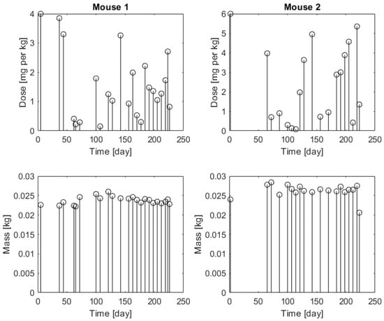
Figure 1.
Injected doses (upper panels) in mg·kg−1 and mice’s weights (bottom panels) in kg (white circle) for Mouse 1 (left panels) and for Mouse 2 (right panels).
The diameter of the tumor mass was measured with a digital clipper.
2.2. Mathematical Model
The model consists of five variables (reported in Table 1) and five equations, of which four are differential and one is algebraic, and 17 parameters (reported in Table 2). Consequently, the model is composed of four compartments: the first two compartments are used to describe the drug pharmacokinetics, the third represents the drug resistance, and the last one is employed for the representation of the tumor cell number.

Table 1.
Model variables along with their units of measurement and physiological meanings.
Table 2.
Model parameters along with their units of measurement and physiological meanings.
In the experiment detailed in Section 2.1, mice were treated with chemotherapy once the tumor volume exceeded a predetermined threshold. Tumor volume was monitored over time, with therapy repeated as needed. During the experiment, some mice exhibited resistance to the treatment, leading to uncontrolled tumor growth. The model describes tumor growth in both resistant and non-resistant mice with the same functional representation; different parameter values give rise to different long-term behavior.
The mathematical formulation is given by the following equations:
where:
- U represents the compartment where the drug is administered;
- Y represents the delay compartment of administered drug;
- Z represents the drug resistance effect;
- X describes the growth of tumor cells;
- V is the tumor volume over time.
Subsequent administrations produce an increase in the variable U of a quantity at time , where is the time of injection of the dose , , with N giving the number of doses and the mass of the mouse at time . Each administered dose occurring after can be represented by a Dirac delta and Equation (1) can be modified as follows:
The Dirac delta function is a simple and effective representation of a rapid increase in the amount of a substance in a specific compartment and its usage is also suggested in [21,23].
Equation (2), coupled with Equation (1) or (6), describes a two-compartment model for drug administration and disposal. The third equation represents the effect of therapy on drug resistance, leading to an accumulation of resistance that impacts tumor cell growth (fourth equation), and, consequently, their remission. While the first term of the Z dynamics represents its increase in dependence on the drug, the second term determines its decrease over time. The exponential term in the fourth equation describes the effect of the resistance on the X size, varying the additional elimination rate between 0 and .
2.3. Parameter Estimation
A parameter estimation procedure was performed using data from the experiments described in the Section 2.1. The model using Equation (6) was adapted to data from two different mice, now referred to as “Mouse 1” and “Mouse 2”. Mouse 1 showed a tumor volume response consistent with therapy sensitivity, whereas Mouse 2’s tumor volume growth suggested the development of resistance. Parameters were estimated by the Ordinary Least Squares method, using a Nelder–Mead optimizer. The Nelder–Mead optimizer, also known as the downhill simplex method, is a numerical technique used to find the minimum or maximum of an objective function in a multidimensional space. It starts with a “simplex”, a shape with n + 1 points in n dimensions (e.g., a triangle in 2D), and through iterative improvements (Reflection, Expansion, Contraction, and Shrinkage) modifies this simplex leading it to an optimal point of the function. This method, which is a direct search method, does not require the calculation of derivatives, making it suitable for optimizing functions that are not differentiable or have discontinuities [24]. Numerical integration was performed via the fixed-step 4-th-order Runge-Kutta method.
The following model parameters were constrained by the experimental design:
- is the starting time for numerical integration.
- is the final time for numerical integration.
- is the tumor mass volume at time .
The parameter , the conversion factor between millions of cells and volume, was determined based on an assumed tumor cell diameter of 6–8 μm. This conversion parameter allows for transforming a specific number of cells (in this case millions of cells) into a total volume.
From this value, parameter , which represents the number of tumor cells at the beginning of the experiment, was computed as (Equation (5)).
The initial conditions , , and for the two mice were set to 0, as therapy administration began after .
The programming language used for the model simulations and parameter estimation was Matlab 2022b [25], running on a Apple computer with an Apple CPU M1 and 8 GB of RAM, needing about 7.4 s to perform a single simulation.
2.4. Stability Analysis
The equilibrium of the system given in Equations (1)–(4) is the solution of
which is the trivial equilibrium point . The Jacobian of the system (1)–(5) is
whose value in the trivial equilibrium becomes
The eigenvalues of the Jacobian evaluated at the equilibrium point are
Since the model parameters are positive, all the eigenvalues are negative real numbers if and only if is negative. As a result, the tumor is stable if the spontaneous elimination rate exceeds the growth rate; thus, no treatment is necessary. The pathological case occurs when the growth rate surpasses the spontaneous elimination rate. In this scenario, the trivial equilibrium becomes unstable, and the tumor requires treatment.
3. Results
Figure 2 shows the observed volume mass, along with the curves estimated by adapting the model to data of the two mice.
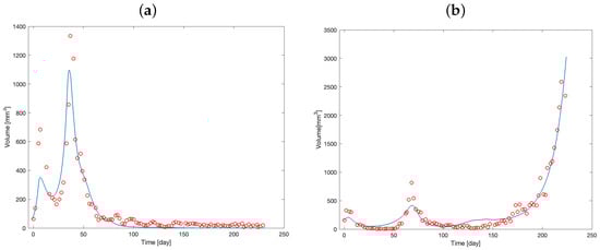
Figure 2.
Tumor mass volume of Mouse 1 (a) and Mouse 2 (b). Red circles represent the observed volume over time; blue solid lines represent the model predictions from the optimization procedure.
The curves demonstrate an initial increase in tumor volume, followed by a decrease after drug administration. In contrast to Figure 2a, Figure 2b illustrates the development of drug resistance in Mouse 2 during the observational period. Initially, the tumor volume decreases following therapy administration, but after approximately day 150, the tumor exhibits exponential growth, indicating the onset of resistance.
Table 3 reports the estimated model parameters in correspondence of the “Free” type row.
Table 3.
Parameters. The table reports the values of model parameters for Mouse 1 and Mouse 2, along with their types: Fixed (not used in the fitting procedure), Free (used in the fitting procedure), Calibrated (subjected to the calibration procedure), and Determined (computed as described in the text).
Figure 3 and Figure 4 show the time course of the administered therapy in the main and delay compartments for the two mice.
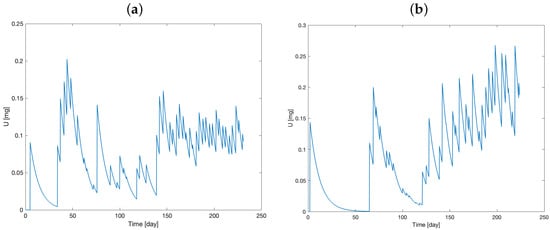
Figure 3.
Model prediction of administered therapy dynamics in main compartment (model variable U) for Mouse 1 (a) and Mouse 2 (b).
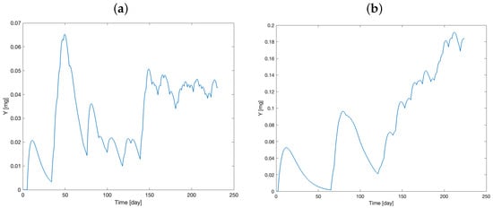
Figure 4.
Model prediction of administered therapy dynamics in delay compartment (model variable Y) for Mouse 1 (a) and Mouse 2 (b).
Initially, the two compartments are set to zero. After drug administration, a rapid increase in the variables can be observed, along with the accumulation of the drug over time.
Figure 5 shows the therapy resistance evolution, while Figure 6 visualizes the number of tumor cells over time.
Figure 5.
Model prediction of the therapy resistance dynamics (model variable Z) for Mouse 1 (a) and Mouse 2 (b).
Figure 6.
Model prediction of the number of tumor cell dynamics (model variable X) for Mouse 1 (a) and Mouse 2 (b).
The curves in Figure 6a,b closely resemble the volume behavior, as the volume is directly dependent on the X variable. These figures depict two distinct responses to the therapy, which are consistent with the time courses illustrated in Figure 5a,b. Specifically, these trends highlight the differing rates at which Mouse 1 and Mouse 2 develop resistance to the therapy.
Figure 2a,b, indeed, suggest greater sensitivity to therapy in Mouse 1 than Mouse 2, which appears to develop resistance to the chemotherapy treatment. The similar estimated values for some parameters between the two mice likely result from the experimental design, which used genetically identical mice and implanted them with the same tumor. For example, the transport rate of the drug from the administration compartment to the delay compartment (parameter ), which is likely independent of therapy susceptibility, was estimated to be d] for Mouse 1 and d] for Mouse 2. In contrast, the estimated parameter values for , , , , and differed substantially between the two mice, reflecting variations in tumor growth and treatment sensitivity. For example, was approximately twice as high in Mouse 1 as in Mouse 2. A smaller , as observed in Mouse 2, leads to sustained levels of Y (Figure 4), which contributes to therapy resistance (increased Z, Figure 5).
Furthermore, the tumor growth rate () was observed to be higher in Mouse 1 compared to Mouse 2. Consistent with expectations, the greatest difference between the two mice was evident in the parameter , which quantifies the therapeutic effect on tumor cell elimination. Mouse 1 demonstrated a markedly higher value for than Mouse 2.
As observed in Section 2.4 above, the stability of the point P only depends on because all the others eigenvalues are negative. Then, if , P is unstable; otherwise, it is stable. It is thus clear that, in the absence of therapy, the stability of the equilibrium point, which translates into the mouse survival, depends only on the difference between these two parameter values. To prove this, a numerical experiment on “Mouse 1” was performed (Figure 7):

Figure 7.
Model simulation of the tumor cell number dynamics with parameter = 0.05 and = 0.1 (a) and = 0.1 and = 0.05 (b).
Figure 7.
Model simulation of the tumor cell number dynamics with parameter = 0.05 and = 0.1 (a) and = 0.1 and = 0.05 (b).

It is possible to observe that the entire dynamics of the system depend on the value of the difference . From an analytical point of view, this occurs because, in the equation
the variable Y is zero, as we hypothesized therapy absence. Therefore, the term is necessarily zero, regardless of the value of Z. For this reason, in the absence of therapy, the system dynamic appears be to completely dependent on the difference .
Figure 8 illustrates the distribution of the relative residuals, calculated as the differences between the observed and predicted volumes divided by the observed volumes, for Mouse 1 (panel a) and Mouse 2 (panel b), respectively.
Figure 8.
Distribution of relative residuals for Mouse 1 (a) and Mouse 2 (b).
The one-sample Kolmogorov–Smirnov test does not confirm the normality of the residuals’ distribution.
4. Discussion
Cyber-medical systems offer a promising approach to revolutionizing cancer treatment through the development of personalized therapies [1,2,3,4,5]. By integrating mathematical models with experimental data, researchers can compare model predictions to actual patient outcomes, identifying key factors influencing treatment response. This enables optimization of drug selection, dosage, and strategies to overcome drug resistance. Ultimately, this personalized approach aims to enhance treatment efficacy and minimize side effects [6,9,10,11,12].
This study presents a novel mathematical model for representing tumor growth in silico. The model was validated using experimental data from a study comparing the growth patterns of tumor cells in genetically identical mice treated with chemotherapy. The results focused on two groups of mice: one with non-resistant tumors and another with resistant tumors. Experimental data from one mouse in each group were used to estimate the model’s parameters. Besides the genetic similarity of the mice, some parameter estimates were similar, due to the common origin of the implanted tumor.
From the validation results, the parameter shows remarkable similarity between the two mice. In two-compartment models, drugs are distributed into central and peripheral compartments, representing plasma/blood and body tissues, respectively. Given the genetic similarity of the mice, it is logical to expect similar pharmacodynamics, leading to comparable values.
The elimination rate of the drug in the delay compartment, , was found to be significantly higher in Mouse 1 (day]) compared to Mouse 2 (d]), resulting in a faster drug clearance in Mouse 1. This difference could be attributed to the higher drug dosage administered to Mouse 2, as shown in Figure 3, if drug elimination, of which the current linear interpretation is just an approximation, was in fact rate-limited. The more rapid drug elimination in Mouse 1 might contribute to a reduced risk of long-term drug resistance.
Another critical parameter is (the tumor growth rate), which turned out to be substantially larger in Mouse 1 than Mouse 2. Although this resulted in more rapid initial tumor growth (Figure 6), it possibly led to Mouse 1 not developing drug resistance in the end, allowing therapy to effectively reduce the tumor mass. Of course, this is just a hypothesis, and more in-depth research is required to evaluate its validity. In contrast, Mouse 2 exhibited a slower tumor growth rate but developed resistance to the drug, rendering the therapy less effective.
While the drug resistance clearance rate () and the drug resistance growth rate () were higher in “Mouse 1”, however, as mentioned above, the key factor determining the development of drug resistance is the difference between these two parameters. In “Mouse 1”, was very large compared to “Mouse 2”, therefore preventing drug resistance.
Finally, the drug effect on the elimination of the tumor, , was, as expected, larger in “Mouse 1” than in “Mouse 2”.
Figure 8 illustrates the model optimization results. For Mouse 1, the overall fit was satisfactory, although the relative error distribution exhibits a mode close to one. This discrepancy arises from the model’s tendency to approach zero during the final observation period (after approximately day 100), while the observed tumor volumes remain small but positive, leading to a peak in the error distribution. For Mouse 2, the model fit was generally good, with the mode of the relative error distribution centered near zero. However, in the rapid growth phase towards the end of the observation period, the model curve slightly underestimates the observed volumes, resulting in negative relative errors. To enhance the accuracy and reliability of the model (diminishing the relative error), future research should address the development of more sophisticated models that move beyond simplified assumptions. This could involve, for example, the explicit differentiation between dead and alive tumor cells, as their distinct contributions to tumor volume and dynamics necessitate separate consideration. Incorporating a dedicated equation to model the therapy effect would allow for a more nuanced representation of treatment responses. Furthermore, accounting for time-varying parameters could be critical for capturing the evolving characteristics of tumor growth. While these refinements inevitably increase the number of parameters requiring estimation, rigorous comparison between parsimonious and complex models, employing statistical methods for model selection, will ultimately deepen our understanding of the underlying physiological mechanisms and improve the predictive power of these models.
The stability analysis reported above also supports the interpretation that most of the meaningful dynamics of the system depend, in the absence of therapy, on the difference . For computational reasons, boundary values were assigned to all variables. As shown in Figure 7b, the variable reaches its boundary, which is a biologically implausible value. In any case, the result is consistent from a medical point of view, where an untreated tumor tends to increase if the “natural elimination factors” (which in the present modelling approach are summarized by the tumor elimination rate ) do not intervene to stop its growth.
The proposed model’s ability to produce results that align with established disease mechanisms, thus providing a clear and insightful picture of the pathophysiology, evidences its robustness. The model effectively differentiates between parameter values associated with the two distinct volume growth behaviors (resistant and non-resistant to therapy). This differentiation underscores the model’s ability to accurately reflect the underlying biological processes.
All the reported figures show not only a good adaptation of the volume model variable to the experimental data, but also plausible behavior of the other model variables. This demonstrates that the proposed formulation provides a valid representation of the tumor growth and of the treatment effect.
Despite the model’s strong performance, several limitations exist. The number of mice used in the estimation procedure was small, and studying a larger population could yield more robust results. Furthermore, the limited number of variables collected in the experiment prevented the investigation of other influential factors, such as stress: several studies have demonstrated that chronic stress can increase the risk of cancer progression and metastasis. Stress likely acts on specific mechanisms that regulate the biology of tumor cells, known as “hallmarks” [26,27]. Another interesting element not considered in the present study was the diet of the subjects, which could have influenced how the mice responded to therapy and/or how the tumors grew over time [28].
5. Conclusions
The model presented in this work is sufficiently simple to represent various therapy conditions without sacrificing information, adapting well to the experimental scenarios. Given its limited number of variables, future studies could benefit from a more comprehensive model that incorporates a wider range of factors influencing tumor growth. Incorporating experimental data from multiple mice could yield a more robust model and enable population parameter estimation, facilitating comparisons between treatment approaches. This would strengthen the model’s reliability and provide insights into the parameter estimates’ confidence. Additionally, integrating further biological factors such as genetic variability, immune response, and micro-environmental influences could significantly enhance the model’s applicability to diverse therapeutic scenarios. This approach would not only improve the precision of parameter estimation but also offer a more holistic understanding of tumor growth dynamics.
Author Contributions
Conceptualization, G.U., M.P., S.P. and A.D.G.; methodology, G.U., M.P., D.A.D. and B.G.; software, G.U. and M.P.; validation, G.U., M.P. and A.D.G.; formal analysis, G.U.; investigation, G.U. and M.P.; resources, S.P. and A.D.G.; data curation, G.U. and M.P.; writing—original draft preparation, G.U., M.P., S.P., D.A.D., B.G. and A.D.G.; writing—review and editing, G.U., M.P., S.P., D.A.D., B.G. and A.D.G.; visualization, M.P. and A.D.G.; supervision S.P. and A.D.G. All authors have read and agreed to the published version of the manuscript.
Funding
This research received no external funding.
Data Availability Statement
The original contributions presented in this study are included in the article. Further inquiries can be directed to the corresponding author.
Acknowledgments
This work was supported by Project PNC 0000001 D3 4 Health—CUP B53C22006100001, The National Plan for Complementary Investments to the NRRP, Funded by the European Union—NextGenerationEU. The work of Andrea De Gaetano was supported by the Distinguished Professor Excellence Program
of Obuda University, Budapest, Hungary.
Conflicts of Interest
The authors declare no conflicts of interest.
References
- Bartoli, G. Il Tumore al Seno e la sua Prevenzione: Una Survey sulla Consapevolezza della Popolazione. Bachelor’s Thesis, Università Politecnica delle Marche, Rome, Italy, 2021. [Google Scholar]
- Agur, Z.; Elishmereni, M.; Kheifetz, Y. Personalizing oncology treatments by predicting drug efficacy, side-effects, and improved therapy: Mathematics, statistics, and their integration. Wiley Interdiscip. Rev. Syst. Biol. Med. 2014, 6, 239–253. [Google Scholar] [CrossRef] [PubMed]
- Taylor, C.A.; Draney, M.T.; Ku, J.P.; Parker, D.; Steele, B.N.; Wang, K.; Zarins, C.K. Predictive medicine: Computational techniques in therapeutic decision-making. Comput. Aided Surg. Off. J. Int. Soc. Comput. Aided Surg. (ISCAS) 1999, 4, 231–247. [Google Scholar] [CrossRef]
- Young, R.A. Biomedical discovery with DNA arrays. Cell 2000, 102, 9–15. [Google Scholar] [CrossRef] [PubMed]
- Singh, H.; Srivastava, H.M. Mathematical Methods in Medical and Biological Sciences; Elsevier Science & Technology: Amsterdam, The Netherlands, 2024. [Google Scholar]
- Boguski, M.S.; Arnaout, R.; Hill, C. Customized care 2020: How medical sequencing and network biology will enable personalized medicine. F1000 Biol. Rep. 2009, 1, 73. [Google Scholar] [CrossRef]
- Butner, J.D.; Dogra, P.; Chung, C.; Pasqualini, R.; Arap, W.; Lowengrub, J.; Cristini, V.; Wang, Z. Mathematical modeling of cancer immunotherapy for personalized clinical translation. Nat. Comput. Sci. 2022, 2, 785–796. [Google Scholar] [CrossRef]
- Kozłowska, E.; Haltia, U.M.; Puszynski, K.; Färkkilä, A. Mathematical modeling framework enhances clinical trial design for maintenance treatment in oncology. Sci. Rep. 2024, 14, 29721. [Google Scholar] [CrossRef]
- Kosorok, M.R.; Laber, E.B. Precision medicine. Annu. Rev. Stat. Its Appl. 2019, 6, 263–286. [Google Scholar] [CrossRef]
- König, I.R.; Fuchs, O.; Hansen, G.; von Mutius, E.; Kopp, M.V. What is precision medicine? Eur. Respir. J. 2017, 50, 1700391. [Google Scholar] [CrossRef]
- Wang, Y.; Wang, N.; Wang, J.; Wang, Z.; Wu, R. Delivering systems pharmacogenomics towards precision medicine through mathematics. Adv. Drug Deliv. Rev. 2013, 65, 905–911. [Google Scholar] [CrossRef][Green Version]
- Barbolosi, D.; Ciccolini, J.; Lacarelle, B.; Barlési, F.; André, N. Computational oncology—Mathematical modelling of drug regimens for precision medicine. Nat. Rev. Clin. Oncol. 2016, 13, 242–254. [Google Scholar] [CrossRef]
- Ochieng, F.O. Mathematical Modeling of Cancerous Tumor Evolution Incorporating Drug Resistance. Eng. Rep. 2025, 7, e70021. [Google Scholar] [CrossRef]
- Kovács, L.; Ferenci, T.; Gombos, B.; Füredi, A.; Rudas, I.; Szakács, G.; Drexler, D.A. Positive Impulsive Control of Tumor Therapy—A Cyber-Medical Approach. IEEE Trans. Syst. Man Cybern. Syst. 2024, 54, 597–608. [Google Scholar] [CrossRef]
- Scolaris, L. Analisi e Modellizzazione Tramite Equazioni Differenziali della Crescita e della Risposta All’immunoterapia del Glioblastoma Multiforme [Analysis and Modellization Using Differential Equations of the Growth and Response to Immunotherapy of Glioblastoma Multiforme]. Ph.D. Thesis, Politecnico di Torino, Torino, Italy, 2024. [Google Scholar]
- Enderling, H.; Chaplain, M.A.; Anderson, A.R.; Vaidya, J.S. A mathematical model of breast cancer development, local treatment and recurrence. J. Theor. Biol. 2007, 246, 245–259. [Google Scholar] [CrossRef] [PubMed]
- Raguz, S.; Yagüe, E. Resistance to chemotherapy: New treatments and novel insights into an old problem. Br. J. Cancer 2008, 99, 387–391. [Google Scholar] [CrossRef]
- Coley, H.M. Mechanisms and strategies to overcome chemotherapy resistance in metastatic breast cancer. Cancer Treat. Rev. 2008, 34, 378–390. [Google Scholar] [CrossRef]
- Pompa, M.; Drexler, D.A.; Panunzi, S.; Gombos, B.; Füredi, A.; Szakács, G.; Kovács, L.; De Gaetano, A. Modeling the development of drug resistance during chemotherapy treatment. In Proceedings of the 2024 IEEE 63rd Conference on Decision and Control (CDC), Milan, Italy, 16–19 December 2024; IEEE: Piscataway, NJ, USA, 2024; pp. 4804–4810. [Google Scholar] [CrossRef]
- Liu, X.; Holstege, H.; van der Gulden, H.; Treur-Mulder, M.; Zevenhoven, J.; Velds, A.; Kerkhoven, R.M.; van Vliet, M.H.; Wessels, L.F.; Peterse, J.L.; et al. Somatic loss of BRCA1 and p53 in mice induces mammary tumors with features of human BRCA1-mutated basal-like breast cancer. Proc. Natl. Acad. Sci. USA 2007, 104, 12111–12116. [Google Scholar] [CrossRef]
- Rottenberg, S.; Nygren, A.O.; Pajic, M.; van Leeuwen, F.W.; van der Heijden, I.; van de Wetering, K.; Liu, X.; de Visser, K.E.; Gilhuijs, K.G.; Van Tellingen, O.; et al. Selective induction of chemotherapy resistance of mammary tumors in a conditional mouse model for hereditary breast cancer. Proc. Natl. Acad. Sci. USA 2007, 104, 12117–12122. [Google Scholar] [CrossRef]
- Füredi, A.; Szebényi, K.; Tóth, S.; Cserepes, M.; Hámori, L.; Nagy, V.; Karai, E.; Vajdovich, P.; Imre, T.; Szabó, P.; et al. Pegylated liposomal formulation of doxorubicin overcomes drug resistance in a genetically engineered mouse model of breast cancer. J. Control. Release 2017, 261, 287–296. [Google Scholar] [CrossRef]
- McNally, A. Using ODEs to Model Drug Concentrations Within the Field of Pharmacokinetics; Augustana College: Rock Island, IL, USA, 2016. [Google Scholar]
- Singer, S.; Singer, S. Efficient implementation of the Nelder–Mead search algorithm. Appl. Numer. Anal. Comput. Math. 2004, 1, 524–534. [Google Scholar] [CrossRef]
- Fernández, M.S.B. MATLAB implementation for evaluation of measurements by the generalized method of least squares. Measurement 2018, 114, 218–225. [Google Scholar] [CrossRef]
- Eckerling, A.; Ricon-Becker, I.; Sorski, L.; Sandbank, E.; Ben-Eliyahu, S. Stress and cancer: Mechanisms, significance and future directions. Nat. Rev. Cancer 2021, 21, 767–785. [Google Scholar] [CrossRef]
- Eng, J.W.L.; Kokolus, K.M.; Reed, C.B.; Hylander, B.L.; Ma, W.W.; Repasky, E.A. A nervous tumor microenvironment: The impact of adrenergic stress on cancer cells, immunosuppression, and immunotherapeutic response. Cancer Immunol. Immunother. 2014, 63, 1115–1128. [Google Scholar] [CrossRef]
- Ho, V.W.; Leung, K.; Hsu, A.; Luk, B.; Lai, J.; Shen, S.Y.; Minchinton, A.I.; Waterhouse, D.; Bally, M.B.; Lin, W.; et al. A low carbohydrate, high protein diet slows tumor growth and prevents cancer initiation. Cancer Res. 2011, 71, 4484–4493. [Google Scholar] [CrossRef] [PubMed]


Disclaimer/Publisher’s Note: The statements, opinions and data contained in all publications are solely those of the individual author(s) and contributor(s) and not of MDPI and/or the editor(s). MDPI and/or the editor(s) disclaim responsibility for any injury to people or property resulting from any ideas, methods, instructions or products referred to in the content. |
© 2025 by the authors. Licensee MDPI, Basel, Switzerland. This article is an open access article distributed under the terms and conditions of the Creative Commons Attribution (CC BY) license (https://creativecommons.org/licenses/by/4.0/).