Article

LV-FeatEx: Large Viewpoint-Image Feature Extraction

1
School of Artificial Intelligence and Computer Science, Jiangnan University, Wuxi 214122, China
2
School of Computing and Augmented Intelligence, Arizona State University, Tempe, AZ 85281, USA
3
Department of Computer Science & Engineering, Xi’an University of Technology, Xi’an 710048, China
*
Authors to whom correspondence should be addressed.
Mathematics 2025, 13(7), 1111; https://doi.org/10.3390/math13071111
Submission received: 25 February 2025 / Revised: 18 March 2025 / Accepted: 22 March 2025 / Published: 27 March 2025

Abstract

:
Maintaining stable image feature extraction under viewpoint changes is challenging, particularly when the angle between the camera’s reverse direction and the object’s surface normal exceeds 40 degrees. Such conditions can result in unreliable feature detection. Consequently, this hinders the performance of vision-based systems. To address this, we propose a feature point extraction method named Large Viewpoint Feature Extraction (LV-FeatEx). Firstly, the method uses a dual-threshold approach based on image grayscale histograms and Kapur’s maximum entropy to constrain the AGAST (Adaptive and Generic Accelerated Segment Test) feature detector. Combined with the FREAK (Fast Retina Keypoint) descriptor, the method enables more effective estimation of camera motion parameters. Next, we design a longitude sampling strategy to create a sparser affine simulation model. Meanwhile, images undergo perspective transformation based on the camera motion parameters. This improves operational efficiency and aligns perspective distortions between two images, enhancing feature point extraction accuracy under large viewpoints. Finally, we verify the stability of the extracted feature points through feature point matching. Comprehensive experimental results show that, under large viewpoint changes, our method outperforms popular classical and deep learning feature extraction methods. The correct rate of feature point matching improves by an average of 40.1 percent, and speed increases by an average of 6.67 times simultaneously.
MSC:
65D18

1. Introduction

Feature point extraction is a fundamental task in computer vision and plays a critical role in supporting various applications based on feature point matching and recognition [1,2,3,4,5]. However, current methods for feature point extraction and description heavily rely on neighborhood information, which becomes unstable under significant viewpoint variations. Such variations cause substantial changes in the neighborhood information around feature points, leading to unreliable feature extraction and, ultimately, matching errors.
To mitigate these challenges, affine-invariant feature extraction methods have been proposed. These methods simulate affine transformations from multiple viewpoints to approximate the camera’s perspective projection, thereby addressing neighborhood variation issues to some extent [6,7,8,9]. For instance, Morel et al. [6] applied affine simulation transformations to images and constructed feature descriptors based on the neighborhood information of feature points. This approach improved the matching rate between similar images before and after viewpoint changes, enhancing the stability of feature point extraction.
Despite these advancements, affine-invariant methods still face critical limitations. Specifically, when the angle between the camera’s viewing direction and the surface normal exceeds 40 degrees (referred to as a “large viewpoint” in this paper), the approximated affine transformations increasingly deviate from the actual perspective projection as viewpoint differences expand. This growing discrepancy causes a rapid deterioration in feature point extraction stability under large viewpoint conditions. Moreover, the exhaustive strategies used in current implementations, which simulate affine transformations from different viewpoints, are computationally expensive and fail to fully compensate for the negative effects of neighborhood changes.
Image feature point extraction consists of two parts: the feature point detector and the feature point descriptor. The feature point detector first compares points in the image and selects their surrounding regions, known as neighborhoods. Based on the neighborhood information, it jointly constructs feature vectors to form feature point descriptors. Researchers have provided many effective solutions to the problem of feature point extraction under conditions of image distortion, noise, and illumination changes [10,11,12,13]. However, it is challenging to achieve stable feature point extraction under large viewpoint changes [14,15].
In recent years, scholars have extensively studied affine-invariant feature point extraction methods. These methods, based on local image features, aim to approximate the extraction of image features under camera perspective transformations. The goal is to adapt to viewpoint changes and improve the robustness of feature point extraction. Among these, ASIFT (Affine-SIFT), proposed by Morel et al. based on SIFT (Scale Invariant Feature Transform) [16], is widely recognized and currently best approximates the camera perspective transformation. The core idea of ASIFT is to construct a set of affine transformations in a discrete viewpoint space. By changing the longitude and latitude angles, it simulates images under different viewpoint changes on the original image. However, this method only uses affine transformation matrices to approximate the scene transformations between two images. It does not truly model the camera’s perspective transformation.
Moreover, the ASIFT method uses SIFT for feature point extraction and requires matching the feature points extracted from each affine-transformed image. This generates a large number of duplicate points, inevitably leading to extra computational overhead and reducing operational efficiency. Additionally, in recent years, many scholars have introduced new feature point extraction methods based on affine simulation strategies. These methods aim to improve the stability of feature point extraction in images from different scenes under large viewpoint changes [17,18,19,20]. Some of these methods have achieved certain improvements in speed compared to ASIFT. However, when performing feature point matching under large viewpoints, the accuracy remains low and is sometimes even reduced further, especially under large viewpoints.
To address this issue, we propose a feature point extraction method more suitable for large viewpoints called LV-FeatEx. As far as we know, this is the first method that directly targets feature point extraction in images with large viewpoints. The method first estimates camera motion parameters under large viewpoint changes based on an optimized affine simulation strategy. Then, it performs inverse perspective transformation on the images using these camera motion parameters, reducing the perspective distortion between the two images. Finally, it applies the SIFT method to extract and match feature points between the two images. Comprehensive experiments verify the more advanced stability of our feature point extraction.
The advantages and innovations of our method are summarized into the following aspects:
  • Feature Point Detector Construction Constrained by a Dual-Threshold: We have developed a detector that uses dual thresholds based on the image grayscale histogram and Kapur’s maximum entropy to constrain AGAST (Adaptive and Generic Accelerated Segment Test) for feature point detection. This approach supports homography estimation and effectively enables more accurate estimation of camera motion parameters.
  • Proposal of an Image Perspective Distortion Correction Method: We introduce a method that constructs a sparser affine simulation transformation model. Using our proposed camera motion parameter estimation method, we perform perspective transformation on images. This not only improves operational efficiency but also reduces the perspective distortion between the two images, enhancing the stability of feature point extraction.

2. Related Work

2.1. The Local Region Normalization Method

The earliest methods of image feature point extraction, countering image viewpoint changes, include Hessian-Affine [21], Harris-Affine [22], and MSER (Maximally Stable Extremal Region) [23]. These methods achieved partial affine invariance by normalizing associated local regions but were only suitable for tasks with small viewpoint variations. To adapt to the task of extracting image feature points under larger viewpoint changes, Morel et al. proposed ASIFT [6]. By exhaustively varying the longitude and latitude angles, it simulates all possible image viewpoints. ASIFT is a milestone method in affine-invariant feature point extraction methods. Compared with SIFT, Harris-Affine, Hessian-Affine, and MSER, ASIFT can better accommodate larger viewpoint changes. SIFT constructs descriptors based on gradient directions and magnitudes in the keypoint neighborhood. Under large viewpoint changes, local gradient distributions undergo substantial shifts. This often leads to descriptor failure. Although ASIFT directly uses SIFT as its feature detector and descriptor, it inherits SIFT’s sensitivity to gradient variations under large viewpoints. The lack of adaptive adjustments for affine-transformed image characteristics results in excessive time complexity from affine simulation. Its ability to handle tilting also remains limited. As a result, a series of improved feature point extraction methods based on SIFT have been proposed, including PCA-SIFT (Principal Component Analysis-SIFT) [24] and SURF (Speeded-Up Robust Features) [25]. To enhance the efficiency of the ASIFT algorithm, Pang et al. [7] combined the SURF algorithm with ASIFT’s affine simulation strategy. They proposed a faster, fully affine-invariant SURF (FAIR-SURF) method. Although the efficiency of SURF in feature point extraction is higher than that of SIFT, it still relies on floating-point descriptors, making it unsuitable for applications with high real-time requirements. Moreover, these methods cannot extract stable feature points when undergoing large viewpoint changes.

2.2. Intensity Feature Point Detector

To enhance the efficiency of feature point extraction, intensity feature detectors have been proposed. Examples include SUSAN (Smallest Univalue Segment Assimilating Nucleus) [26], FAST (Features from Accelerated Segment Test) [27], FAST-ER (FAST Enhanced Repeatability) [28], and AGAST [29]. These methods simplify image gradient computations by comparing the intensity of the central pixel with that of surrounding pixels. Among these, AGAST is an improvement over FAST and is currently one of the best. It defines two additional pixel brightness comparison criteria. AGAST improves the speed of feature point extraction by searching for the optimal decision tree in an expanded structural space. It also combines accelerated segmentation algorithms to maintain the accuracy of existing methods. It performs better than FAST. However, the threshold in the AGAST algorithm needs to be manually set, which limits its adaptability in different environments. In addition, to achieve faster feature descriptor matching speeds, binary descriptors like BRIEF (Binary Robust Independent Elementary Features) [30], ORB (Oriented FAST and Rotated BRIEF) [31], BRISK (Binary Robust Invariant Scalable Keypoints) [32], FREAK (Fast Retina Keypoint) [33], AKAZE (Accelerated-KAZE) [34], LATCH (Learned Arrangements of Three Patch Codes) [35], and BEBLID (Boosted Efficient Binary Local Image Descriptor) [36] have been proposed. Among these methods, FREAK performs better. It compares image intensities sampled according to a human retina sampling pattern, achieving fast computation and low memory cost while maintaining robustness to scaling, rotation, and noise. However, most of these binary descriptor methods can only perform feature point extraction under small viewpoint changes. Therefore, to more quickly extract invariant features under large viewpoint changes, Ma et al. [16] combined the intensity-based FAST feature detector and binary FREAK descriptor with the ASIFT affine simulation strategy, proposing the fully affine-invariant AFREAK (Affine-FREAK) algorithm. This allows the FREAK descriptor to describe feature points under large viewpoint changes. FREAK’s fixed retinal sampling pattern cannot dynamically adapt to large viewpoint deformations. This results in unpredictable bit flips in the binary descriptor, reducing robustness. Additionally, AFREAK inherits ASIFT’s exhaustive search of affine parameters, leading to high computational costs that fail to meet real-time requirements. Hou et al. [8] combined the ORB algorithm with the ASIFT affine simulation strategy and proposed the AORB (Affine-ORB) algorithm; however, it still suffers from the limitations of the manually set threshold in the ORB feature detection algorithm. In summary, methods that improve ASIFT using intensity-based feature detectors and binary descriptors have achieved some speed improvements but at the expense of accuracy. This is especially problematic under large viewpoint changes, where the issue of high computational time for image feature point extraction becomes even more severe. Moreover, the inherent vulnerability of binary descriptors to geometric deformations makes it difficult to maintain stable feature matching under large viewpoint transformations.

2.3. Deep Learning Feature Point Extraction Methods

In recent years, with the rapid development of deep learning, researchers have proposed many learning-based feature point extraction methods [37,38,39,40]. However, when extracting feature points under large viewpoint changes or in scenes with severe deformations, existing convolutional neural network (CNN)-based methods face challenges. Due to perspective transformations caused by camera motion, the local features to be extracted are altered. As a result, deep convolutional techniques struggle to describe the spatially stable relationships between two similar features under large viewpoint changes [41].

3. Methodology

3.1. Overview of Framework

Existing methods for extracting feature points under large viewpoint changes share a common characteristic: they require exhaustive extraction of feature points from a large number of images taken from different viewpoints. Then, they search for similar images to perform feature point matching. This leads to extremely high time complexity, and even more inaccuracy because of the error propagation. The core motivation of our framework lies in addressing the trade-off between computational efficiency and robustness in large viewpoint changes by integrating sparse affine simulation with adaptive thresholding, which distinguishes our method from existing brute-force matching approaches.
If the transformation matrix between the two images was known in advance, it could directly replace the exhaustive matching process. This would improve both the speed and accuracy of the method. To this end, we draw on the idea of affine simulation from ASIFT. While ASIFT achieves affine invariance through dense sampling, its computational redundancy limits practical applicability. Our key innovation lies in redesigning the sampling strategy to balance coverage and efficiency, which is critical for real-time scenarios. By sparsely optimizing the longitude sampling points in the affine simulation, we estimate the transformation matrix between images. Using this matrix, we align the perspective distortions between the two images with viewpoint changes. This effectively eliminates the viewpoint transformation between images, enhancing the stability of feature point extraction under large viewpoint changes.
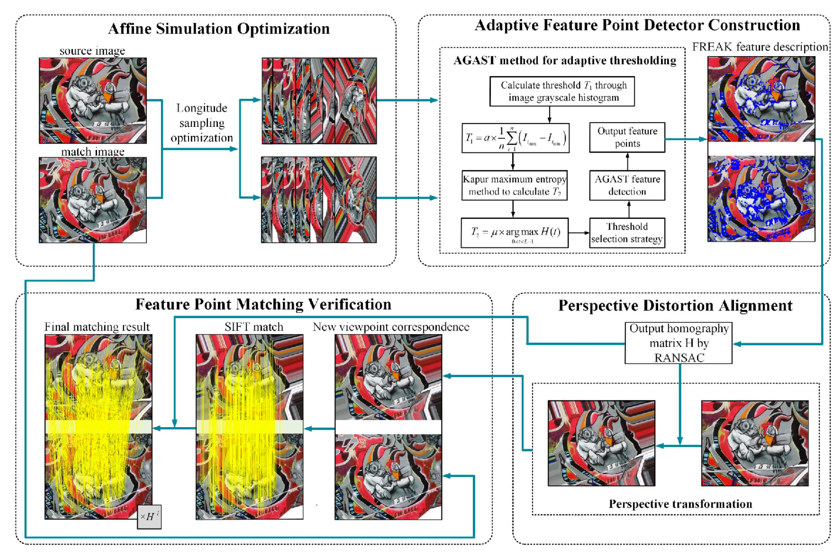
The overall framework of our method is shown in Figure 1. It includes four components: affine simulation optimization, adaptive feature point detector construction, perspective distortion alignment, and feature point matching verification. The uniqueness of our framework stems from the synergistic design of these components: (1) affine simulation optimization reduces redundancy while preserving critical viewpoints, (2) adaptive thresholding dynamically balances feature quantity and quality, (3) perspective distortion alignment leverages homography estimation for distortion correction, and (4) SIFT-based verification ensures robustness. This integration addresses limitations of isolated module improvements in prior works.
First, based on the affine simulation strategy, we designed a sparser affine simulation model by adjusting the step size of longitude sampling. Then, utilizing the grayscale information of the images and incorporating Kapur’s maximum entropy method, we designed an adaptive AGAST [29] feature point detector that supports dual thresholds.
Next, based on the FREAK [27] descriptor, we used the homography matrix H . This matrix, generated by the Random Sample Consensus (RANSAC) algorithm [42], was used to perform an inverse perspective transformation on the source image. Finally, by applying the inverse of the homography matrix, we transformed the SIFT matching points from the transformed image back to the original image, thereby verifying the stability of feature point extraction.
Below are descriptions of the details of each part, including affine simulation optimization, adaptive feature point extraction, perspective distortion elimination, and feature point matching verification.

3.2. Affine Simulation Optimization

Affine-invariant feature point extraction can be considered an extension of scale-invariant feature point extraction to handle non-uniform scaling and tilting. This means that there are different scaling factors in two orthogonal directions, and angles are not preserved.
Non-uniform scaling not only affects position and scale but also the local feature structures of the image. Therefore, scale-invariant feature point extraction methods fail under significant affine transformations.
The affine camera model is represented by the matrix shown in Equations (1)–(6).
A = B C D E F
B = 1 0 t x 0 1 t y 0 0 1
C = cos ψ sin ψ 0 sin ψ cos ψ 0 0 0 1
D = s 0 0 0 s 0 0 0 1
E = 1 / cos θ 0 0 0 1 0 0 0 1
F = cos ϕ sin ϕ 0 sin ϕ cos ϕ 0 0 0 1
t x and t y are the translation variables in the x and y directions, ψ is the camera’s rotation variable, s is the uniform scaling factor, ϕ is the longitude, and θ is the latitude. These two variables define the direction of the camera’s principal optical axis.
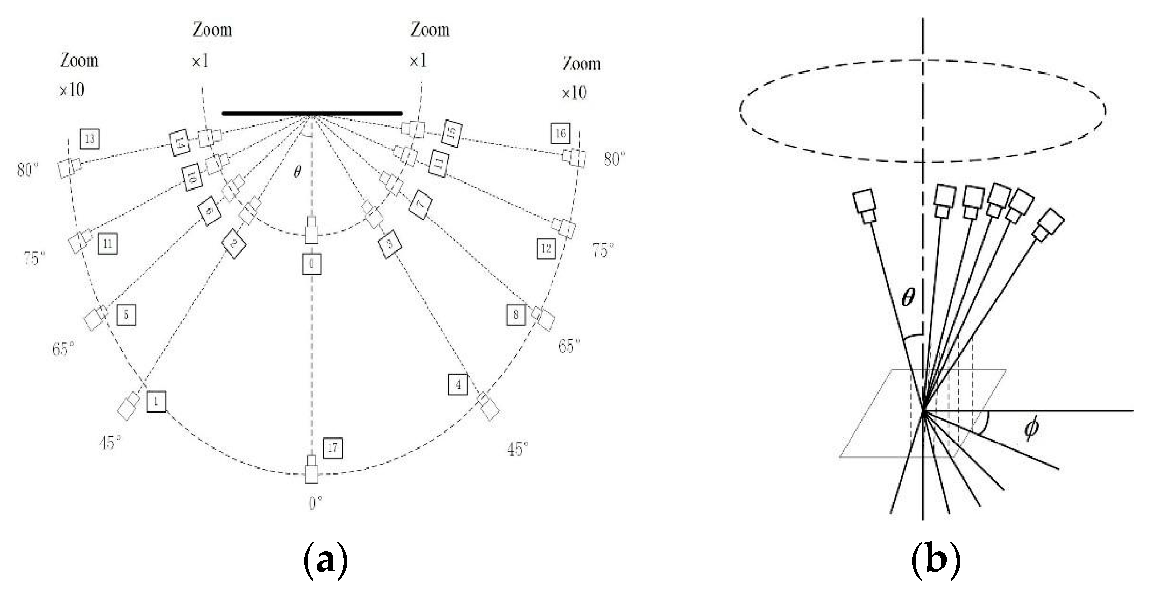
Therefore, the viewpoint changes caused by camera movement when capturing the same object can be approximated with an affine transformation model. This model helps simulate the effects of different viewpoints. By adjusting the latitude and longitude angles, the affine transformation simulates images from different viewpoints. The observation hemisphere of these angles is shown in Figure 2. The black dots in the figure represent sampling points at various latitudes and longitudes. Corresponding simulated images with affine deformation can be generated based on the affine matrix. Refer to the following description for the sampling rules of the latitude angle θ and longitude angle ϕ .
1.
The latitude angle θ = arccos ( 1 / t ) , where θ and t have a one-to-one correspondence. The tilt corresponding to θ can be t = 1 ,   a ,   a 2 ,   a n with a = 2 ;
2.
The longitude angle ϕ and t have a one-to-many relationship, with ϕ = 72 ° / t . k is a positive integer that satisfies ϕ < 180 ° and Δ ϕ = 72 ° / t .
Based on the one-to-many relationship between the parameter t and the longitude angle ϕ , it can be seen that the value of ϕ significantly affects the time complexity of affine transformations. When t [ 2 ,   2 ,   2 2 ,   4 ,   4 2 ] , the sampling points before optimization are shown in Figure 3a, where the values of Δ ϕ at different latitudes are Δ ϕ = 50 ° ,   36 ° ,   25 ° ,   18 ° ,   12 ° , with a total of 42 sampling points. For affine simulation, the smaller the value of Δ ϕ , the more identical information is contained in the simulated images, and the more feature points can be extracted from the simulated images, resulting in more matched feature points.
However, since this paper applies affine simulation to estimate camera motion parameters under large viewpoint changes, it is not necessary to have a large number of matching points during this process. Having too many feature points would create redundancy in the feature information and increase computational cost. This would not significantly improve the estimation of camera motion parameters. The goal of the affine simulation optimization strategy in this section is to enhance the efficiency of feature point extraction during affine simulation. It also aims to cover as many different viewpoints as possible, supporting efficient camera motion parameter estimation under large viewpoint changes.
Therefore, to balance the accuracy and time complexity of the feature point extraction method in this paper, the step size for longitude sampling is increased to reduce redundant sampling points and achieve optimization. The optimized 12 sampling points are shown in Figure 3b, where the values of Δ ϕ at different latitudes are Δ ϕ = 181 ° ,   128 ° ,   90 ° ,   64 ° ,   45 ° The one-to-many relationship between the optimized t and Δ ϕ can be expressed as: Δ ϕ = 256 ° / t .
As shown in Figure 3b, optimizing the longitude sampling significantly reduces the number of simulated viewpoint samples. Despite this reduction, the optimized sampling still effectively covers the affine simulations of different viewpoints. It meets the requirements for camera motion parameter estimation and reduces the computational time overhead of affine simulation.

3.3. Adaptive Feature Point Detector Construction

In this section, we utilize AGAST [29] for feature point detection. In AGAST, the threshold represents the minimum contrast between potential feature point locations and their surrounding pixels. A higher threshold leads to fewer detected feature points; conversely, a lower threshold results in more feature points. Because the AGAST algorithm requires manual threshold setting, these fixed thresholds cannot meet the demands of different scenarios. To address this issue, we introduce a dual-threshold constraint during feature point extraction. This approach enables adaptive threshold setting for the AGAST algorithm and simultaneously extracts initial feature points to support subsequent homography matrix estimation.
3.
Setting of Threshold T1
We determine the dynamic threshold T 1 of the AGAST algorithm based on the degree of variation in image grayscale contrast. Specifically, we first set the vertical axis range of the histogram. This range represents the frequencies of different grayscale values. It was set to [0, 255] as the basis for calculating the threshold in the next step. This serves as the basis for calculating the threshold in the next step. Then, we sample the i grayscale values that appear most frequently and least frequently. The dynamic threshold T 1 is defined as shown in Equation (7).
T 1 = a × 1 n i = 1 n I i max I i min
where I i min and I i max   i = ( 1 , 2 , 3 , , n ) represent the i grayscale values that appear the least and the most in the image, respectively, and a is the proportional coefficient. In the experiments of this paper, n is set to 10, and a is set to 0.3.
4.
Setting of Threshold T2
It is insufficient to merely use the variation in image grayscale values as a threshold constraint for the AGAST algorithm. When an image has weak texture features but strong brightness variations, relying solely on the grayscale histogram to set the AGAST threshold can result in unreasonable threshold settings. This may lead to an insufficient number of feature points being detected. Therefore, we introduce a dynamic threshold T2 to further constrain the AGAST algorithm’s threshold. We adopt Kapur’s maximum entropy method [43,44] to determine T2. This method uses conditional probabilities to describe the grayscale distributions of the image’s foreground and background, thereby defining their respective entropies.
In the following, we use an 8-bit grayscale image as an example for illustration. Accordingly, the grayscale range in this algorithm is represented as ( 0 ,   1 ,   ,   L 1 ) , where L = 256 . The image is divided into foreground and background based on a threshold. The foreground consists of pixels with grayscale values greater than or equal to the threshold, while the background comprises pixels with grayscale values less than the threshold. Therefore, each pixel in the image belongs either to the foreground or to the background. Therefore, under the threshold T , the image is divided into two subclasses S b = { 0 ,   1 ,   ,   t } and S f = { t + 1 ,   ,   L 1 } . At this point, the entropy of the image includes the background entropy component H ( S b ) and the foreground entropy component H ( S f ) , as shown in Equations (8) and (9)
H S b = H t P t + ln P t
H ( S f ) = H n H t 1 P t + ln ( 1 P t )
where H n is the entropy of the image, defined as H n = i = 0 L 1 p i ln p i , P t = i = 0 t p i and H t = i = 0 t p i ln p i . p i represents the probability density p i = n i N . N represents the total number of pixels, N = i = 0 L 1 n i . n i represents the number of pixels with a grayscale value of i .
H ( t ) = H ( S b ) + H ( S f )         = ln P t ( 1 P t ) + H t P t + H n H t 1 P t
Equation (10) represents the entropy of the entire image under a certain threshold segmentation. Using the image histogram, the maximum entropy for image threshold segmentation is calculated. The algorithm traverses the grayscale range of the image (0 to 255), computing the entropy value at each grayscale level. The threshold value T is the one that maximizes the entropy H of the image. This threshold T is then selected for segmentation. That is T = arg   max   0 < t < L 1 H ( t ) , where the optimal threshold T 2 is given by Equation (11).
T 2 = a × T
where a is the proportional coefficient. Since the threshold of the feature points is related to the image contrast, Kapur’s maximum entropy method is used to identify the points where the grayscale variation in the image is most significant.
Suppose the coordinates of a pixel on the image are ( x , y ) , and the grayscale value at that point is I ( x , y ) . In the AGAST algorithm, the pixel will only be selected as a feature point if the grayscale values of the n   ( n = 16 ) pixels on the Bresenham circle around it are all greater than I ( x , y ) + T or all less than I ( x , y ) T (where T is the threshold, set as T 1 or T 2 in practical applications).
It is worth noting that the affine simulation strategy proposed by Morel et al. [7] only varies two variables in the affine transformation matrix. This requires that the feature point extraction algorithm used in affine simulation must satisfy the remaining four degrees of freedom in the model. Since the SIFT algorithm possesses translation, rotation, and scale invariance, ASIFT achieves full affine invariance. Similarly, the binary descriptor FREAK also has strong translation, rotation, and scale invariance. Therefore, in this paper, we use the adaptive AGAST feature detection method combined with the FREAK feature descriptor. This combination highlights the adaptive nature of the initial feature point extraction. Moreover, our algorithm significantly outperforms the ASIFT algorithm in terms of execution efficiency.

3.4. Perspective Distortion Alignment

Unlike existing methods based on affine simulation strategies, in this subsection we first estimate the camera motion parameters between two image frames. Then, we eliminate the perspective distortion between the images to reduce the impact of viewpoint changes. Finally, we perform extraction and matching of the final feature points on images adjusted for the new viewpoint relationship.
To estimate the camera motion parameters between two images, it is necessary to detect at least four pairs of matching feature points sufficient to solve the homography matrix. Therefore, in the camera motion estimation stage, the extracted feature points (initial feature points) are required to be successfully matched, and the matching points should be few but precise. This goal is achieved by combining the previously optimized longitude simulation sampling model and an adaptive-threshold AGAST detector. Specifically, we use the adaptive AGAST feature detector for initial feature point detection. These points are then described and matched using the FREAK descriptor, enabling rapid estimation of camera motion parameters.
Perspective transformation is based on the pinhole imaging principle used in conventional cameras. It maps objects from the world coordinate space to the image coordinate space. The inverse perspective transformation is its reverse operation. Perspective transformation can more accurately reflect the viewpoint changes between two images captured during camera motion. Assuming the camera moves from the viewpoint position of the matched image to that of the source image, the perspective transformation between the two images can be performed based on the homography transformation matrix between them. This provides a reliable opportunity for distortion correction.
Therefore, we estimate the camera’s perspective transformation parameters based on affine simulated sampling. This approach is equivalent to obtaining a more precise 3 × 3 perspective transformation matrix from matched point pairs derived from 13 pairs of simulated views, each using 2 × 3 affine transformation matrices. Therefore, we can utilize the initial feature point correspondences obtained through the affine simulation strategy. Using the homography matrix generated by the RANSAC algorithm with findHomography() in OpenCV, we perform an inverse perspective transformation on the target image. This allows us to achieve perspective alignment between the two images.

3.5. Feature Point Extraction and Matching Verification

By aligning the perspective-distorted images in 
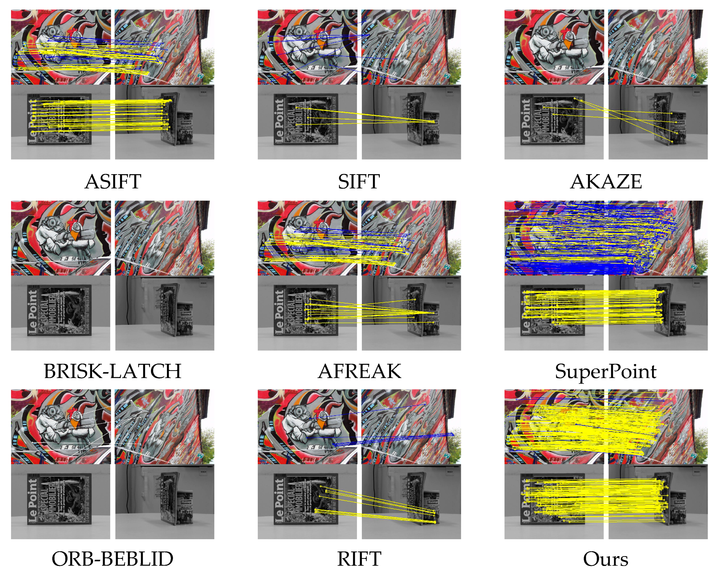
Section 3-D, we obtained a new viewpoint relationship. This alignment reduces or effectively eliminates the inconsistencies between the two images caused by viewpoint transformations. Consequently, the stability of matching based on feature point descriptors is enhanced. Furthermore, we selected SIFT, considered the “gold standard” [45], to perform feature point extraction and matching verification on the image pairs with the new viewpoint relationship.
Since one image from the source image underwent an inverse perspective transformation relative to another image (as shown in Figure 4), the viewpoint relationship between the original image pairs has changed. The original viewpoint correspondence and the new viewpoint correspondence are shown in Figure 4a,b, respectively. As a result, the two images in the new viewpoint pair are effectively aligned under the same perspective transformation standard (by multiplying with the inverse homography matrix H 1 ). This alignment enhances the stability of feature extraction and matching.

4. Experimental Results and Analysis

4.1. Complexity Theory Analysis

We compare the proposed method with SIFT, ASIFT, and AFREAK algorithms in terms of time complexity.
Assume the input image size is W × H , the number of feature points is n , the number of sampling points for a single image in ASIFT is k o r i g , and the number of sampling points after affine simulation optimization using our method is k o p t .
The SIFT algorithm involves two stages of feature extraction and one brute-force matching process. The computational cost of SIFT feature extraction and matching is expressed in Equation (12).
T S I F T = 2 O ( W H log W H ) + O ( n 2 )
The ASIFT algorithm involves multiple affine simulations and SIFT processing steps. The computational cost of ASIFT feature extraction and matching is expressed in Equation (13).
T A S I F T R = 2 k o r i g O ( W H log W H ) + k o r i g 2 O ( n 2 )
The AFREAK algorithm involves FAST keypoint detection, affine simulation, and FREAK descriptor generation. The computational cost of AFREAK feature extraction and matching is expressed in Equation (14).
T A F R E A K = O ( W H ) + O ( n ) + O ( n 2 )
Based on the sampling rules and experimental settings of this paper, the actual computational cost of the proposed method is expressed in Equation (15).
T o u r = O ( k o p t W H log W H ) + O ( k o p t n 2 ) + O ( m n )
Compared to ASIFT, the proposed method demonstrates significant superiority in terms of time efficiency. It greatly simplifies the steps and reduces the time required for feature extraction and matching, resulting in a lower computational cost and significantly improving the method’s real-time performance. The experimental results are consistent with our analysis.
Compared to AFREAK, the proposed method reduces affine simulation complexity by decreasing the number of sampling points. By employing dynamic threshold control and using an adaptive AGAST detector, it reduces redundant feature points n , alleviating the actual cost of O ( n 2 ) . Additionally, geometric alignment acceleration, combined with inverse perspective transformation and RANSAC, further enhances matching efficiency. The experimental results validate the correctness of the theoretical analysis and the effectiveness of the optimization strategies.

4.2. Datasets

The experiment in this paper uses the HPatches dataset [46], specifically the image set with viewpoint variations (providing up to 60 ° of viewpoint changes). This dataset presents images of various real-world scenes under different viewpoint transformations. Each HPatches image set consists of six images in sequence. All subsequent images are transformations of the first image, with each having a different degree of viewpoint change relative to the first. For the v_graffiti and v_bricks image subsets, HPatches draws from the Oxford Affine Dataset [47], where the images are generated by gradually increasing the tilt angle from 10° to 60°, thereby introducing challenges to feature point extraction. For the v_adam, v_bird, and v_grace image subsets, HPatches applies three settings—EASY, HARD, and TOUGH—to challenge feature detection.
To test the impact of larger viewpoint changes on the method, this paper also uses the Morel dataset [7] to measure the amount of distortion between one view and another. The data collection process is shown in Figure 5. This dataset includes two sampling methods: absolute tilt sampling, which provides images with viewpoint changes up to 80°, and transitional tilt sampling, which provides images with viewpoint changes up to 90°. Specifically, in the absolute tilt sampling shown in Figure 5a, the viewpoint angle between the camera’s optical axis and the object’s surface normal changes from 0° (front view) to 80°, with intervals between 1 and 10°. In the transitional tilt sampling shown in Figure 5b, the distance and latitude angle θ are fixed, while the longitude angle ϕ is varied from 0° to 90° during the image capture process.

4.3. Evaluation Metrics

This paper uses the following evaluation criteria: Number of Feature Point Matches (NFPM), Correct Matching Rate (CMR), Root Mean Square Error (RMSE) and the overall execution time of the method.
  • Number of Feature Point Matches
The NFPM is used as an indicator to evaluate the robustness of the proposed feature point extraction method. In this paper, it refers to the number of feature point matches obtained after outliers are removed through the ratio test and the RANSAC algorithm.
2.
Correct Matching Rate
CMR is defined as the ratio of correctly matched points to the total number of feature point matches, as shown in Equation (16).
C M R = c o r r e c t   m a t c h e s N F P M
where correct matches refer to the correctly matched points based on homography estimation, and NFPM refers to the number of feature point matches.
In addition, the correct matches are calculated using the given ground truth matrix H . Let ( x , y ) and ( x , y ) be the matching point pairs. According to the dataset’s given ground truth matrix H , they are evaluated using Equation (17). When the pixel error between the matching points after homography estimation projection is less than 3 , the matching point pair is considered correct.
( H x x ) 2 + ( H y y ) 2 < 3
where ( x , y ) and ( x , y ) are the matching points in the images, and H is the ground truth matrix.
3.
Root Mean Square Error
RMSE refers to the precise error value for each pair of matched points at the pixel level [48]. Let ( x i , y i ) and ( x i , y i ) be the coordinates of the i -th matched feature point pair. The calculation of RMSE is shown in Equation (18).
R M S E = 1 N F P M i = 1 N F P M [ ( x i x i ˜ ) 2 + ( y i y i ˜ ) 2 ]
where ( x ˜ i , y ˜ i ) represents the coordinates of ( x i , y i ) after transformation using the ground truth matrix.
4.
Overall execution time
The overall execution time of the method was used as the evaluation index of the performance of the algorithm. In order to reflect the stability of the experimental results, the algorithm was executed 10 times for each pair of images and the average value was taken as the final result.

4.4. Experimental Results

Figure 6a,b shows the trends in the NFPM and CMR of the proposed method across different image sets as the viewpoint changes. The experimental results, evaluated using RMSE and overall method execution time on different image sets, are shown in Figure 6c,d. The RMSE represents the cumulative value across images with different viewpoints in the entire image set. The experimental results on the HPatches dataset, evaluated using CMR and overall method execution time, are shown in Figure 7.
As shown in Figure 6a, although the NFPM decreases as the viewpoint angle increases in the HPatches image set, there are still enough matching point pairs. Combining the CMR in Figure 6b and the RMSE values in Figure 6c, it can be seen that the proposed method achieves both a high CMR and high accuracy. From Figure 6b, it is evident that, in most scenarios with viewpoint changes, the method demonstrates relatively stable CMR performance as the viewpoint angle increases. Even under large viewpoint changes, the method performs well.
From Figure 6d, it can be observed that, as the viewpoint changes, the overall runtime of the method remains roughly consistent at each image tilt angle. However, for certain images, the overall runtime differs significantly compared to other images.
For example, when processing images from the v_graffiti dataset at a 60° tilt angle, the overall runtime of the method is significantly higher compared to images at other viewpoints. This is because the adaptive threshold settings of AGAST vary on images with different grayscale characteristics. Specifically, at a 60° tilt in the v_graffiti dataset, a lower AGAST feature point detection threshold is set due to the grayscale properties of the images. This leads to an increase in the NFPM and consequently extends the overall runtime of the method. In the case of the v_bird dataset at a 60° tilt angle, the CMR decreases noticeably, and the runtime also decreases. This is because the similarity between the tilted images and the original images in the v_bird dataset drops sharply at 60°, resulting in a reduction of the NFPM.
The following experiment is conducted on the Morel dataset. Since the dataset itself does not provide a ground truth matrix, only the NFPM and the overall execution time of the method are evaluated. The NFPM as the viewpoint changes is shown in Figure 7. Additionally, the average overall execution time of the proposed method is 233.9 ms for absolute tilt and 237.55 ms for transitional tilt.

4.5. Ablation Study

In this subsection, two types of comparisons were conducted in the ablation experiments. First, we compared the effects of setting different thresholds for AGAST within our method to those of our adaptive AGAST threshold. Second, we evaluated the impact on our method’s performance with and without the application of affine optimization. The experiments were conducted on the v_graffiti image set from the HPatches dataset.
First, we observe the impact of setting different AGAST thresholds during the camera motion parameter estimation stage on the CMR and the method’s overall execution time. The thresholds tested were 35, 40, 45, 50, and 55, as well as the adaptive threshold used in this paper. The experimental results under different evaluation criteria are shown in Table 1.
The threshold of the AGAST feature detector affects both the CMR and the method’s overall execution time. A lower threshold increases the NFPM that needs to be calculated, thus increasing the overall execution time. Raising the threshold beyond 45 has little effect on the overall execution time. However, the CMR decreases noticeably at thresholds of 35 and 55. The adaptive threshold used in this paper achieves optimal performance in terms of both CMR and overall execution time.
As shown in Table 1, setting different thresholds for the AGAST detector has varying impacts on CMR and the overall execution time of the method. From the perspective of execution time, the larger the threshold, the shorter the time required. However, the effect on CMR is not directly proportional, making it difficult to manually find an optimal threshold for the AGAST feature detector. In contrast, the adaptive threshold designed in this paper achieves optimal performance in both execution time and CMR. Therefore, the adaptive AGAST threshold strategy proposed in this paper holds significant importance.
To accurately assess the effectiveness of the affine simulation optimization strategy, we design two sets of experiments: the Affine Simulation Optimization Application Group and the Affine Simulation Optimization Ablation Group. In the application group, the complete method is implemented, including affine simulation optimization. In contrast, the ablation group uses an unoptimized affine simulation strategy. All other conditions between the two experiments are kept consistent to ensure the reliability and comparability of the results.
This paper comprehensively evaluates the performance of the method in the two experimental groups, focusing on the evaluation metrics such as the NFPM, CMR, RMSE, and the method’s overall execution time. The experimental results for the different evaluation criteria are shown in Table 2. It can be observed that after applying the affine simulation optimization the NFPM remains almost unchanged, while RMSE decreases. The affine simulation optimization strategy used in this paper significantly reduces the method’s overall execution time and improves CMR.
Overall, the proposed affine simulation optimization strategy improves both execution time and CMR compared to the original strategy. The NFPM remains almost unchanged, even as the viewpoint angle of the images varies. Therefore, the affine simulation optimization strategy proposed in this paper holds significant importance.

4.6. Parameter Variation Experiment

This section’s parameter variation experiment involves setting different values for the feature point detection threshold parameter a in the proposed method. The goal is to explain why a is set to 0.3 in this paper. The experiment is conducted on the v_graffiti image set from the HPatches dataset.
To investigate the impact of setting different values for a in the proposed method, a parameter variation experiment was conducted on the v_graffiti image set. The main evaluation metrics considered were the NFPM, CMR, RMSE, and the method’s overall execution time. The experimental results for different evaluation criteria are shown in Table 3. The values of a were tested from 0.1 to 0.9 to observe their effect on the final feature point extraction results.
As seen from Table 3, as a increases, the overall execution time first decreases and then increases. This is because when a = 0.1 , a = 0.2 , and a = 0.3 , the T 1 threshold is used. When a exceeds 0.3, the T 2 threshold is applied, leading to feature point extraction using two thresholds, which increases the time cost. Based on the data in Table 3, the method performs optimally when a = 0.3 , and thus this value is selected as the threshold parameter in this paper.

4.7. Experimental Comparison and Analysis

In this section, a comparative analysis is conducted between the proposed method and several other methods, including ASIFT [6], SIFT [10], AKAZE [34], BRISK-LATCH [35], AFREAK [16], SuperPoint [38], ORB-BEBLID [34], and RIFT [3]. Among these, SuperPoint is a CNN-based method, and the pretrained model provided in the original paper (Outdoor) is used for the network. For this comparison, the classic v_graffiti and v_grace image sets were selected to evaluate the methods.

4.7.1. Matching Results Under Different Viewpoints

First, Figure 8 shows a comparison of the matching results for different methods under a 60° viewpoint in the v_graffiti image set from the HPatches dataset. It also presents the results under an 80° viewpoint in the absolute tilt image set from the Morel dataset. For the v_graffiti image set, yellow lines represent correct matching point pairs, while blue lines represent incorrect matches. For the Morel image set, since no validation matrix is provided, only the matching points are shown using yellow lines. From the matching result comparison in Figure 8, it can be observed that the ASIFT and AFREAK methods show an excessive concentration of feature points, with many redundant points included. In contrast, the feature points extracted by the proposed method are more evenly distributed. Additionally, under a 60° viewpoint change, methods like SIFT, AKAZE, ORB-BEBLID, and RIFT perform poorly or even fail to match. Although the SuperPoint method appears to have enough matching points, many of them are incorrect. In terms of matching performance, the feature points extracted by the proposed method are superior in both the uniformity of point distribution and the number of correct matches. Moreover, the proposed method performs exceptionally well under large viewpoint changes.

4.7.2. Experimental Results Using CMR Metric

Figure 9 shows the experimental results from the v_graffiti and v_grace image subsets of the HPatches dataset, using CMR as the evaluation metric. The line charts in Figure 9a,b illustrate the variation in CMR across different methods as the viewpoint changes in the v_graffiti and v_grace image sets. Figure 10 reflects the change in the NFPM as the viewpoint changes. Table 4 and Table 5 present a comparison of the average CMR, total NFPM, RMSE, and the overall execution time of different methods on the v_graffiti and v_grace image subsets. In the tables, if RMSE is marked with an asterisk (*), it indicates that the method failed to match certain image pairs in that image set.

4.7.3. CMR Performance Analysis

As shown in Figure 9, in the v_graffiti and v_grace image sets, the SIFT, AKAZE, BRISK-LATCH, and ORB-BEBLID methods perform well when the viewpoint change is small, with their best performance at a 20° viewpoint change. However, as the viewpoint angle increases, the CMR rapidly decreases, eventually reaching zero. RIFT performs poorly on the v_graffiti image set. ASIFT and AFREAK, due to their affine invariance, maintain relatively stable performance under viewpoint changes, but their CMR is lower than SIFT when the viewpoint change is small. SuperPoint can successfully match under large viewpoint changes, but its overall CMR is relatively low.
In contrast, the proposed method achieves an even higher CMR compared to SIFT, AKAZE, BRISK-LATCH, and ORB-BEBLID under small viewpoint changes. It also maintains a high CMR under large viewpoint changes. From the average CMR metrics in Table 4 and Table 5, the proposed method demonstrates the best performance among the compared methods, with more stable and reliable results.

4.7.4. NFPM Performance Analysis

As shown in Figure 10, SIFT, AKAZE, BRISK-LATCH, and ORB-BEBLID methods have a relatively high NFPM (Number of Feature Point Matches) at 20° and 30° viewpoint changes. However, as the viewpoint angle increases, the NFPM rapidly decreases, and feature point matching fails at 50° and 60° viewpoints. Although ASIFT and AFREAK methods have a higher NFPM than the proposed method in the first two images of the v_graffiti dataset, their NFPM also drops quickly as the tilt angle of the image increases. While the SuperPoint method maintains a relatively stable NFPM as the viewpoint changes, its match count is lower than that of the proposed method, and the matching examples show many incorrect matches.
The proposed method exhibits a more gradual decrease in the NFPM as feature point extraction becomes more challenging. It maintains enough matching points even under maximum difficulty. Although the proposed method has the highest NFPM in the v_grace image set, it does not have the highest NFPM in the v_graffiti image set. However, when considering the CMR and RMSE metrics from Table 4 and Table 5 (with numbers in parentheses indicating the rank within the same column), the proposed method achieves the most correct matches and the highest matching accuracy. It shows good stability under large viewpoint changes. This makes it suitable for practical applications like 3D reconstruction, which require both precision and a large number of feature point matches.

4.7.5. Execution Time Performance Comparison

The experimental results in Table 4 and Table 5 evaluate the overall runtime performance on the v_graffiti and v_grace image sets from the HPatches standard dataset. Our method has an average processing time lower than ASIFT, AFREAK, BRISK-LATCH, SuperPoint, and RIFT. On the v_graffiti image set, it is comparable to the ORB-BEBLID method and slightly higher than SIFT and AKAZE. In the v_grace image set, our method is on par with SIFT and slightly exceeds AKAZE and ORB-BEBLID.
However, SIFT, AKAZE, and ORB-BEBLID perform poorly under large viewpoint changes. In contrast, similar to ASIFT, AFREAK, and SuperPoint, our method effectively extracts feature points under significant viewpoint changes. It does so with relatively low computational costs. The richer the features in the images, the more pronounced the speed advantage of our method becomes.

4.7.6. Improvements in CMR and RMSE Metrics

In terms of CMR, our method shows significant improvements compared to other methods. The average CMR on the v_graffiti dataset increased by 42.05%, while on the v_grace dataset, it rose by 38.06%. Regarding RMSE (only compared with successful matching methods), our method reduced the average error by 5.38 pixels on the v_graffiti image set and by 5.23 pixels on the v_grace image set, indicating higher matching accuracy.
From the analysis of the above experiments, our method has a slightly longer overall runtime than AKAZE, ORB-BEBLID, and SIFT. However, the performance metrics for CMR, NFPM, and RMSE indicate that this time cost is acceptable. Moreover, our method successfully performs feature point extraction and matching under significant viewpoint changes. This demonstrates better performance compared to AKAZE, ORB-BEBLID, and SIFT. Additionally, when compared to other feature extraction methods that can handle large viewpoint changes, our method achieves a higher CMR and greater computational efficiency. It improves the overall runtime by an average of 6.12 times on the v_graffiti dataset and by 7.21 times on the v_grace dataset.

4.7.7. Performance Validation on the Morel Dataset

We validated the effectiveness of our method under larger viewpoint changes using the Morel dataset. The Morel dataset does not provide the homography matrix for perspective transformations during camera motion. As a result, we cannot calculate the true coordinates of the matched feature points. Therefore, we are unable to obtain the CMR and RMSE metrics. In this study, we used overall execution time and the NFPM as evaluation standards. The experimental results based on the NFPM are presented in Table 6 and Table 7. The results based on overall runtime are shown in Table 8. It is evident that our method still performs well under larger viewpoint changes. The overall execution time is slightly higher than that of AKAZE, ORB-BEBLID, and SIFT. However, our method achieves feature point extraction under significant viewpoint changes with minimal time cost when considering the NFPM. This is consistent with the conclusions drawn from the experiments on the HPatches dataset. It is worth noting that this paper also compares the deep learning-based feature point extraction method SuperPoint, which is trained on homography datasets. Compared to AKAZE, SIFT, RIFT, BRISK-LATCH, and ORB-BEBLID, SuperPoint is better suited for feature point extraction on images with large viewpoint changes. However, its performance in terms of CMR and the NFPM is not as good as the proposed method, and it requires significantly higher computational resources.

5. Conclusions

This paper proposes a feature point extraction method, LV-FeatEx, for images under large viewpoint changes. The proposed method employs optimized affine simulation to achieve perspective-distortion-aligned feature point extraction, enhancing stability under large viewpoints. Comprehensive experimental results show that the proposed method increases average matching accuracy by 40.1% compared to several classic feature point extraction and deep learning-based methods. It also improves speed by 6.67 times, achieving high performance in both accuracy and speed.
The method streamlines camera parameter estimation and integrates the more efficient FREAK descriptor to enhance efficiency. However, when the image undergoes large rotations, the FREAK descriptor’s ability to support feature matching decreases. As the tilt angle increases, the number of feature point matches decreases significantly. Especially after 60 degrees, the NFPM drops sharply, indicating a substantial reduction in the number of feature points extracted and matched by the algorithm under larger viewpoint changes. The correct match rate also shows a noticeable decline after 60 degrees, suggesting that the matching accuracy of the algorithm is affected under larger viewpoint changes.

Author Contributions

Conceptualization, Y.W. (Yukai Wang), Y.W. (Yinghui Wang) and W.L.; methodology, Y.W. (Yukai Wang) and W.L.; software, Y.W. (Yukai Wang), W.L. and Y.L.; validation, Y.L. and L.H.; investigation, Y.W. (Yukai Wang); data curation, Y.W. (Yukai Wang) and Y.L.; writing—original draft preparation, Y.W. (Yukai Wang); writing—review and editing, Y.W. (Yinghui Wang) and X.N.; visualization, W.L.; supervision, Y.W. (Yinghui Wang); project administration, Y.W. (Yinghui Wang); funding acquisition, Y.W. (Yinghui Wang) All authors have read and agreed to the published version of the manuscript.

Funding

This work was supported by the National Key Research and Development Program (No. 2023YFC3805901), in part of the National Natural Science Foundation of China (No. 62172190), in part of the “Double Creation” Plan of Jiangsu Province (Certificate: JSSCRC2021532), and in part of the “Taihu Talent-Innovative Leading Talent Team” Plan of Wuxi City (Certificate Date: 202412).

Data Availability Statement

The data presented in this study are openly available in HPatches at 10.1109/CVPR.2017.410, reference number 46. Additional experimental data can be obtained by contacting the corresponding author.

Conflicts of Interest

The authors declare that there are no conflicts of interest in this article.

References

  1. Liu, X.; Zhao, X.; Xia, Z.; Feng, Q.; Yu, P.; Weng, J. Secure Outsourced SIFT: Accurate and Efficient Privacy-Preserving Image SIFT Feature Extraction. IEEE Trans. Image Process. 2023, 32, 4635–4648. [Google Scholar] [PubMed]
  2. Xia, Y.; Ma, J. Locality-Guided Global-Preserving Optimization for Robust Feature Matching. IEEE Trans. Image Process. 2022, 31, 5093–5108. [Google Scholar] [CrossRef] [PubMed]
  3. Chen, Y.; Xiao, Y.; Wu, H.; Chen, C.; Lin, D. Multi-Scale Geometric Feature Extraction and Global Transformer for Real-World Indoor Point Cloud Analysis. Mathematics 2024, 12, 3827. [Google Scholar] [CrossRef]
  4. Pei, Y.; Dong, Y.; Zheng, L.; Ma, J. Multi-Scale Feature Selective Matching Network for Object Detection. Mathematics 2023, 11, 2655. [Google Scholar] [CrossRef]
  5. Shen, X.; Hu, Q.; Li, X.; Wang, C. A Detector-Oblivious Multi-Arm Network for Keypoint Matching. IEEE Trans. Image Process. 2023, 32, 2776–2785. [Google Scholar] [CrossRef]
  6. Morel, J.M.; Yu, G. ASIFT: A new framework for fully affine invariant image comparison. SIAM J. Imaging Sci. 2009, 2, 438–469. [Google Scholar]
  7. Pang, Y.; Li, W.; Yuan, Y.; Pan, J. Fully affine invariant SURF for image matching. Neurocomputing 2012, 85, 6–10. [Google Scholar] [CrossRef]
  8. Hou, Y.; Zhou, S.; Lei, L.; Zhao, J. Fast fully affine invariant image matching based on ORB. Comput. Eng. Sci. 2014, 36, 303–310. [Google Scholar]
  9. Kostková, J.; Suk, T.; Flusser, J. Affine invariants of vector fields. IEEE Trans. Pattern Anal. Mach. Intell. 2019, 43, 1140–1155. [Google Scholar]
  10. Lowe, D.G. Distinctive image features from scale-invariant keypoints. Int. J. Comput. Vis. 2004, 60, 91–110. [Google Scholar] [CrossRef]
  11. Winarni, S.; Indratno, S.W.; Arisanti, R.; Pontoh, R.S. Image Feature Extraction Using Symbolic Data of Cumulative Distribution Functions. Mathematics 2024, 12, 2089. [Google Scholar] [CrossRef]
  12. Sa, J.; Zhang, X.; Yuan, Y.; Song, Y.; Ding, L.; Huang, Y. A Novel HPNVD Descriptor for 3D Local Surface Description. Mathematics 2025, 13, 92. [Google Scholar] [CrossRef]
  13. Yu, Y.; Huang, K.; Chen, W.; Tan, T. A novel algorithm for view and illumination invariant image matching. IEEE Trans. Image Process. 2011, 21, 229–240. [Google Scholar] [PubMed]
  14. Tu, Y.; Li, L.; Su, L.; Du, J.; Lu, K.; Huang, Q. Viewpoint-Adaptive Representation Disentanglement Network for Change Captioning. IEEE Trans. Image Process. 2023, 32, 2620–2635. [Google Scholar] [CrossRef]
  15. Chang, Y.; Xu, Q.; Xiong, X.; Jin, G.; Hou, H.; Man, D. SAR image matching based on rotation-invariant description. Sci. Rep. 2023, 13, 14510. [Google Scholar] [CrossRef] [PubMed]
  16. Ma, X.; Liu, D.; Zhang, J.; Xin, J. A fast affine-invariant features for image stitching under large viewpoint changes. Neurocomputing 2015, 151, 1430–1438. [Google Scholar] [CrossRef]
  17. Nan, B.; Wang, Y.; Liang, Y.; Wu, M.; Qian, P.; Lin, G. Ad-RSM: Adaptive Regional Motion Statistics for Feature Matching Filtering. In Proceedings of the CGI 2022 (Computer Graphics International 2022), Online, 12–16 September 2022. [Google Scholar]
  18. Huang, F.-C.; Huang, S.-Y.; Ker, J.-W.; Chen, Y.-C. High-Performance SIFT Hardware Accelerator for Real-Time Image Feature Extraction. IEEE Trans. Circuits Syst. Video Technol. 2012, 22, 340–351. [Google Scholar] [CrossRef]
  19. Yang, E.; Chen, F.; Wang, M.; Cheng, H.; Liu, R. Local Property of Depth Information in 3D Images and Its Application in Feature Matching. Mathematics 2023, 11, 1154. [Google Scholar] [CrossRef]
  20. Wang, N.N.; Wang, B.; Wang, W.P.; Guo, X.H. Computing Medial Axis Transform with Feature Preservation via Restricte Power Diagram. ACM Trans. Graph. 2022, 41, 188. [Google Scholar] [CrossRef]
  21. Mikolajczyk, K.; Schmid, C. An affine invariant interest point detector. In Proceedings of the Computer Vision—ECCV 2002: 7th European Conference on Computer Vision, Copenhagen, Denmark, 28–31 May 2002; Volume 2350, pp. 128–142. [Google Scholar]
  22. Mikolajczyk, K.; Schmid, C. Scale & Affine Invariant Interest Point Detectors. Int. J. Comput. Vis. 2004, 60, 63–86. [Google Scholar]
  23. Matas, J.; Chum, O.; Urban, M.; Pajdla, T. Robust wide-baseline stereo from maximally stable extremal regions. Image Vis. Comput. 2004, 22, 761–767. [Google Scholar]
  24. Ke, Y.; Sukthankar, R. PCA-SIFT: A more distinctive representation for local image descriptors. In Proceedings of the 2004 IEEE Computer Society Conference on Computer Vision and Pattern Recognition, 2004. CVPR 2004, Washington, DC, USA, 27 June–2 July 2004; p. II. [Google Scholar]
  25. Bay, H.; Ess, A.; Tuytelaars, T.; Van Gool, L. Speeded-up robust features (SURF). Comput. Vis. Image Underst. 2008, 110, 346–359. [Google Scholar] [CrossRef]
  26. Smith, S.M.; Brady, J.M. SUSAN—A new approach to low level image processing. Int. J. Comput. Vis. 1997, 23, 45–78. [Google Scholar]
  27. Trajković, M.; Hedley, M. Fast corner detection. Image Vis. Comput. 1998, 16, 75–87. [Google Scholar] [CrossRef]
  28. Rosten, E.; Porter, R.; Drummond, T. Faster and Better: A Machine Learning Approach to Corner Detection. IEEE Trans. Pattern Anal. Mach. Intell. 2010, 32, 105–119. [Google Scholar] [CrossRef]
  29. Mair, E.; Hager, G.D.; Burschka, D.; Suppa, M.; Hirzinger, G. Adaptive and generic corner detection based on the accelerated segment test. In Proceedings of the Computer Vision–ECCV 2010: 11th European Conference on Computer Vision, Heraklion, Greece, 5–11 September 2010; Proceedings, Part II 11. Springer: Berlin/Heidelberg, Germany, 2010; pp. 183–196. [Google Scholar]
  30. Calonder, M.; Lepetit, V.; Strecha, C.; Fua, P. Brief: Binary robust independent elementary features. In Proceedings of the Computer Vision–ECCV 2010: 11th European Conference on Computer Vision, Heraklion, Greece, 5–11 September 2010; Proceedings, Part IV 11. Springer: Berlin/Heidelberg, Germany, 2010; pp. 778–792. [Google Scholar]
  31. Rublee, E.; Rabaud, V.; Konolige, K.; Bradski, G. ORB: An efficient alternative to SIFT or SURF. In Proceedings of the 2011 IEEE International Conference on Computer Vision, Barcelona, Spain, 6–13 November 2011; pp. 2564–2571. [Google Scholar]
  32. Leutenegger, S.; Chli, M.; Siegwart, R.Y. BRISK: Binary Robust invariant scalable keypoints. In Proceedings of the 2011 International Conference on Computer Vision, Barcelona, Spain, 6–13 November 2011; pp. 2548–2555. [Google Scholar]
  33. Alahi, A.; Ortiz, R.; Vandergheynst, P. FREAK: Fast Retina Keypoint. In Proceedings of the 2012 IEEE Conference on Computer Vision and Pattern Recognition, Providence, RI, USA, 16–21 June 2012; pp. 510–517. [Google Scholar]
  34. Alcantarilla, P.F.; Solutions, T. Fast explicit diffusion for accelerated features in nonlinear scale spaces. IEEE Trans. Pattern Anal. Mach. Intell. 2011, 34, 1281–1298. [Google Scholar]
  35. Levi, G.; Hassner, T. LATCH: Learned arrangements of three patch codes. In Proceedings of the 2016 IEEE Winter Conference on Applications of Computer Vision (WACV), Lake Placid, NY, USA, 7–10 March 2016; pp. 1–9. [Google Scholar]
  36. Suárez, I.; Sfeir, G.; Buenaposada, J.M.; Baumela, L. BEBLID: Boosted efficient binary local image descriptor. Pattern Recognit. Lett. 2020, 133, 366–372. [Google Scholar]
  37. DeTone, D.; Malisiewicz, T.; Rabinovich, A. Superpoint: Self-supervised interest point detection and description. In Proceedings of the IEEE Conference on Computer Vision and Pattern Recognition Workshops, Salt Lake City, UT, USA, 18–22 June 2018; pp. 224–236. [Google Scholar]
  38. Sarlin, P.E.; DeTone, D.; Malisiewicz, T.; Rabinovich, A. Superglue: Learning feature matching with graph neural networks. In Proceedings of the IEEE/CVF Conference on Computer Vision and Pattern Recognition, Seattle, WA, USA, 14–19 June 2020; pp. 4938–4947. [Google Scholar]
  39. Xue, X.; Guo, J.; Ye, M.; Lv, J. Similarity Feature Construction for Matching Ontologies through Adaptively Aggregating Artificial Neural Networks. Mathematics 2023, 11, 485. [Google Scholar] [CrossRef]
  40. Wang, C.; Ning, X.; Li, W.; Bai, X.; Gao, X. 3D Person Re-Identification Based on Global Semantic Guidance and Local Feature Aggregation. IEEE Trans. Circuits Syst. Video Technol. 2024, 34, 4698–4712. [Google Scholar]
  41. Ma, J.; Jiang, X.; Fan, A.; Jiang, J.; Yan, J. Image Matching from Handcrafted to Deep Features: A Survey. Int. J. Comput. Vis. 2021, 129, 23–79. [Google Scholar]
  42. Fischler, M.A.; Bolles, R.C. Random sample consensus: A paradigm for model fitting with applications to image analysis and automated cartography. Commun. ACM 1981, 24, 381–395. [Google Scholar] [CrossRef]
  43. Kapur, J.N.; Sahoo, P.K.; Wong, A.K.C. A new method for gray-level picture thresholding using the entropy of the histogram. Comput. Vis. Graph. Image Process. 1985, 29, 273–285. [Google Scholar] [CrossRef]
  44. Upadhyay, P.; Chhabra, J.K. Kapur’s entropy based optimal multilevel image segmentation using crow search algorithm. Appl. Soft Comput. 2020, 97, 105522. [Google Scholar] [CrossRef]
  45. Bellavia, F. SIFT matching by context exposed. IEEE Trans. Pattern Anal. Mach. Intell. 2022, 45, 2445–2457. [Google Scholar] [CrossRef]
  46. Balntas, V.; Lenc, K.; Vedaldi, A.; Mikolajczyk, K. HPatches: A benchmark and evaluation of handcrafted and learned local descriptors[C]. In Proceedings of the IEEE Conference on Computer Vision and Pattern Recognition, Honolulu, HI, USA, 21–26 July 2017; pp. 5173–5182. [Google Scholar]
  47. Mikolajczyk, K.; Tuytelaars, T.; Schmid, C.; Zisserman, A.; Matas, J.; Schaffalitzky, F.; Kadir, T.; Gool, L.V. A comparison of affine region detectors. Int. J. Comput. Vis. 2005, 65, 43–72. [Google Scholar] [CrossRef]
  48. Kupfer, B.; Netanyahu, N.S.; Shimshoni, I. An efficient SIFT-based mode-seeking algorithm for sub-pixel registration of remotely sensed images. IEEE Geosci. Remote Sens. Lett. 2014, 12, 379–383. [Google Scholar] [CrossRef]
Figure 1. Technical Framework Diagram of the Method.
Mathematics 13 01111 g001
Figure 2. Observation Hemisphere Diagram for Affine Simulated Sampling (Only show t = 2 ,   2 2 ,   4 ).
Mathematics 13 01111 g002
Figure 3. Top View of Simulated Sampling Points. (a) Affine Simulated Sampling Points Used in ASIFT; (b) Simulated Sampling Points of the Proposed Method.
Mathematics 13 01111 g003
Figure 4. Example of Viewpoint Transformation Correspondence. (a) Original Viewpoint Relationship; (b) New Viewpoint Relationship.
Mathematics 13 01111 g004
Figure 5. Examples of Absolute Tilt and Transitional Tilt Camera Sampling. (a) Absolute Tilt Sampling; (b) Transitional Tilt Sampling.
Mathematics 13 01111 g005
Figure 6. Comparison of Evaluation Metric Changes on the HPatches Dataset. (a) NFPM; (b) CMR; (c) RMSE; (d) Overall Execution Time.
Mathematics 13 01111 g006
Figure 7. NFPM Experimental Results on the Morel Dataset. (a) Absolute Tilt; (b) Transitional Tilt.
Mathematics 13 01111 g007
Figure 8. A comparison of feature point extraction and matching results on datasets under different viewpoints. The evaluated methods include ASIFT [6], SIFT [10], AKAZE [34], BRISK-LATCH [35], AFREAK [16], SuperPoint [38], ORB-BEBLID [34], and RIFT [3]. In the first row, the HPatches dataset is used with a maximum viewing angle of 60 degrees. In the second row, the Morel dataset is used with a maximum viewing angle of 80 degrees. In the figures, blue lines indicate incorrect matches, while yellow lines represent correct matches.
Mathematics 13 01111 g008
Figure 9. CMR Experimental Results of Different Methods on the v_graffiti and v_grace Image Sets. (a) v_graffiti Image Sets; (b) v_grace Image Sets.
Mathematics 13 01111 g009
Figure 10. NFPM Experimental Results of Different Methods on the v_graffiti and v_grace Image Sets. (a) v_graffiti Image Sets; (b) v_grace Image Sets.
Mathematics 13 01111 g010
Table 1. Comparison of Evaluation Metric Values for Different AGAST Threshold Settings.
AGAST ThresholdNFMP↑CMR↑RMSE↓Overall Execution Time (ms)↓
35336491.33%4.731485.38
40340893.13%4.722492.28
45344393.66%4.575453.93
50347592.30%4.644441.22
55330191.57%4.768417.41
Adaptive337593.73%4.535399.44
Bold values denote the optimal results under the same experimental conditions. Arrows indicate desired direction of metrics (↑: higher is better, ↓: lower is better).
Table 2. Comparison of Evaluation Metric Values Based on Whether Affine Simulation Optimization is Applied.
MethodNFMP↑CMR↑RMSE↓Overall Execution Time (ms)↓
Performing Affine Simulation337593.73%4.536395.14
Without Affine Simulation342292.55%4.7081244.58
Bold values denote the optimal results under the same experimental conditions. Arrows indicate desired direction of metrics (↑: higher is better, ↓: lower is better).
Table 3. Comparison of Evaluation Metric Values for Different a Settings on the v_graffiti Image Set.
Parameter aNFMP↑CMR↑RMSE↓Overall Execution Time (ms)↓
a = 0.1337192.68%4.709773.72
a = 0.2341093.47%4.644687.24
a = 0.3337593.72%4.535395.14
a = 0.4328992.13%4.691566.59
a = 0.5348291.59%4.732593.50
a = 0.6333891.83%4.794567.25
a = 0.7324692.65%4.822573.81
a = 0.8331192.71%4.633606.64
a = 0.9342392.74%4.676576.03
Bold values denote the optimal results under the same experimental conditions. Arrows indicate desired direction of metrics (↑: higher is better, ↓: lower is better).
Table 4. Comparison of Evaluation Metric Values for Different Methods on the v_graffiti Image Set.
MethodNFMP↑CMR↑RMSE↓Overall Execution Time (ms)↓
ASIFT [6]3805 (1)78.35%7.2762996.69
SIFT [10]136476.32%*201.40 (2)
AKAZE [34]93441.76%*123.82 (1)
BRISK-LATCH [35]51524.12%*704.87
AFREAK [16]3751 (2)87.17%6.2841206.10
ORB-BEBLID [34]155944.72%*384.10 (3)
RIFT [3]635.0%*9949.10
SuperPoint [38]292156.00%16.1843046.24
Ours3375 (3)93.73%4.536395.14 (4)
Bold values denote the optimal results under the same experimental conditions. Arrows indicate desired direction of metrics (↑: higher is better, ↓: lower is better). If RMSE is marked with an asterisk (*), it indicates that the method failed to match certain image pairs in that image set.
Table 5. Comparison of Evaluation Metrics for Different Methods on the v_grace Image Set.
MethodNFMP↑CMR↑RMSE↓Overall Execution Time (ms)↓
ASIFT [6]685281.68%6.6128772.15
SIFT [10]322049.67%*643.63 (3)
AKAZE [34]220241.76%*123.82 (1)
BRISK-LATCH [35]148224.12%*704.87 (4)
AFREAK [16]557884.42%5.9881863.34
SuperPoint [3]493876.90%12.7934767.56
ORB-BEBLID [38]288867.80%*402.51 (2)
RIFT [34]70657.14%*14,473.2
Ours689581.68%3.237712.52 (5)
Bold values denote the optimal results under the same experimental conditions. Arrows indicate desired direction of metrics (↑: higher is better, ↓: lower is better). If RMSE is marked with an asterisk (*), it indicates that the method failed to match certain image pairs in that image set.
Table 6. NFPM Statistics for Different Methods Under Absolute Tilt Testing on the Morel Dataset (zoom = 4).
Absolute Tilt AngleASIFT [6] SIFT [10]AKAZE [34]BRISK-LATCH [35]AFREAK [16]SuperPoint [38] ORB-BEBLID [34]RIFT [3]Ours
10°1225987103114491357729160215331101
20°117595696813871215715144313571080
30°931780686978830492109210321024
40°569682422227507592497671885
50°57331014848393505105172726
60°3847713101843871136586
70°23884490301415440
80°504401717609103
Total514538043276410345934097475448255945
Bold values denote the optimal results under the same experimental conditions.
Table 7. NFPM Statistics for Different Methods Under Transitional Tilt Testing on the Morel Dataset (zoom = 2).
Transitional Tilt AngleASIFT [6] SIFT [10]AKAZE [34]BRISK-LATCH [35]AFREAK [16]SuperPoint [38] ORB-BEBLID [34]RIFT [3]Ours
10°7454383753061364355668271555
20°48311536276303375118532
30°4383213543731987495
40°23476024730408510
50°27464024528147483
60°23454016825307396
70°2129501422006405
80°1755001412209398
90°19254412333017324
Total2987622447342349719247313504098
Bold values denote the optimal results under the same experimental conditions.
Table 8. Overall Execution Time of Different Methods on the Morel Dataset (Unit:ms).
MethodASIFT [6] SIFT [10]AKAZE [34]BRISK-LATCH [35]AFREAK [16]SuperPoint [38] ORB-BEBLID [34]RIFT [3]Ours
Absolute Tilt3009.44186.1782.79458.99424.36329.24121.515725.13233.90
Transitional Tilt3088.62201.6768.14429.45573.69210.22216.475309.24237.55
Bold values denote the optimal results under the same experimental conditions.
Disclaimer/Publisher’s Note: The statements, opinions and data contained in all publications are solely those of the individual author(s) and contributor(s) and not of MDPI and/or the editor(s). MDPI and/or the editor(s) disclaim responsibility for any injury to people or property resulting from any ideas, methods, instructions or products referred to in the content.

