Abstract
To address the challenges of distribution cost and efficiency in electric vehicle (EV) logistics, this study proposes a time-dependent, multi-center, semi-open heterogeneous fleet model. The model incorporates a nonlinear power consumption measurement framework that accounts for vehicle parameters and road impedance, alongside an objective function designed to minimize the total cost, which includes fixed vehicle costs, driving costs, power consumption costs, and time window penalty costs. The self-organizing mapping network method is employed to initialize the EV routing, and an improved adaptive large neighborhood search (IALNS) algorithm is developed to solve the optimization problem. Experimental results demonstrate that the proposed algorithm significantly outperforms traditional methods in terms of solution quality and computational efficiency. Furthermore, through real-world case studies, the impacts of different distribution modes, fleet sizes, and charging strategies on key performance indicators are analyzed. These findings provide valuable insights for the optimization and management of EV distribution routes in logistics enterprises.
Keywords:
electric vehicle path problem; improved adaptive large neighborhood search algorithm; heterogeneous fleet; time-dependent; multi-center MSC:
90B06; 90B50; 68W10
1. Introduction
With the development of China’s urban logistics industry, the use of fossil energy increases year by year, which leads to environmental pollution. Electric vehicle distribution has the advantage of “low energy consumption, low pollution.” “Low energy consumption” refers to minimal use of energy resources, while “low pollution” indicates reduced emission of harmful substances. Together, they describe environmentally-friendly practices that minimize energy use and environmental impact, crucial for sustainable development and ecological preservation. For this reason, some logistics enterprises began to use electric vehicle distribution. However, electric vehicles are limited by their short driving range and susceptibility to urban time-varying road networks. During large-scale distribution processes, drivers often experience “range anxiety.” Range anxiety refers to the psychological stress experienced by electric vehicle (EV) drivers due to concerns about insufficient battery range to complete a trip or reach the next charging station. This phenomenon is particularly relevant in urban logistics, where frequent stops and varying traffic conditions can exacerbate range uncertainty. This anxiety results in the underutilization of battery capacity. In addition, with the diversification of people’s demand for commodities, distribution centers need to send out vehicles of different sizes according to the types of products demanded, the amount of customer demand and other factors, which further increases the difficulty of optimizing the distribution path of electric vehicles. Therefore, in the process of distribution services, rational planning of vehicle paths and distribution modes, as well as the adoption of appropriately configured fleets and charging strategies, have become urgent problems to be solved.
The electric vehicle routing problem (EVRP) is an extension of the classical vehicle routing problem (VRP) and focuses on optimizing delivery routes for electric vehicles (EVs) while considering their unique characteristics, such as limited battery capacity, energy consumption rates, charging station locations, and charging time requirements. The primary objective is to minimize total delivery costs while ensuring that vehicles can complete their routes without running out of charge, often incorporating constraints related to charging infrastructure, vehicle range, and time windows for customer deliveries. Numerous scholars have conducted research on various variants of this problem. Schneider et al. [1] studied the electric vehicle routing problem with time windows and charging stations. Ahmed et al. [2] investigated the vehicle routing problem with time windows and proposed a hybrid ant colony optimization algorithm for its resolution. Jiang et al. [3] addressed the issue that charging navigation cannot simultaneously optimize the charging destination and route planning for electric vehicles. They established a bi-level stochastic optimization model for electric vehicle charging navigation that considers multiple uncertainty factors and proposed a hierarchical enhanced deep Q network-based method to solve the aforementioned stochastic optimization model. He et al. [4] considered the electric vehicle routing problem with multi-temperature co-distribution and proposed a mathematical model with soft time windows. They improved the ant colony optimization algorithm by incorporating the 2-opt algorithm, and experimental results showed that this method effectively reduces delivery costs and improves delivery efficiency. Veena et al. [5] focused on charging prices and proposed a time-of-use pricing-based efficient electric vehicle routing optimization method using the bat algorithm, aiming to reduce electricity costs and total travel distance.
With the gradual advancement of research, numerous scholars have begun to explore more variants of the electric vehicle routing problem (EVRP) to address urban logistics distribution challenges. For instance, some researchers have focused on heterogeneous fleet distribution strategies. The heterogeneous fleet distribution strategy involves the use of a mixed fleet of vehicles with varying capacities, energy source, and operational characteristics. This strategy enables logistics enterprises to tailor vehicle assignments based on specific delivery requirements, thereby improving efficiency, reducing costs, and supporting sustainable practices. Wang et al. [6] constructed an integer programming model considering mixed fleets to solve the “last mile” delivery issue in rural logistics. Afsane et al. [7] established a mixed-integer programming model for route selection involving conventional and hybrid fleets in urban logistics distribution and employed an adaptive large neighborhood search (ALNS) algorithm for solution. Wang et al. [8] investigated the heterogeneous fleet vehicle routing problem for hazardous materials and solved it using an adaptive fuzzy large neighborhood search algorithm. Sarbijan et al. [9] developed a multi-type vehicle routing optimization model under mid-route replenishment scenarios and utilized a particle swarm optimization algorithm combined with simulated annealing for solving. Sun et al. [10] proposed a multi-vehicle collaborative segmented transshipment model to improve the efficiency of fresh product distribution, employing the k-means clustering algorithm to determine transshipment points and an adaptive multi-objective ant colony optimization algorithm for solution. The aforementioned studies predominantly adopted single-center distribution models or multi-center closed models. To address large-scale customer distribution challenges, some scholars have shifted their focus to multi-center semi-open vehicle routing problems. The semi-open distribution model refers to a logistics strategy where vehicles are allowed to return to the nearest distribution center after completing their delivery tasks, rather than being restricted to their original departure point. This approach reduces travel distances, optimizes resource utilization, and enhances operational flexibility, particularly in large-scale distribution networks. For such problems, Nistha et al. [11] investigated a multi-center vehicle routing problem for surplus food redistribution and solved it using an elite genetic algorithm. Alaia et al. [12] treated the multi-vehicle, multi-depot, semi-open vehicle routing problem with time windows as a multiple-criteria optimization problem and applied a genetic algorithm with elite selection strategies. Nunes et al. [13] resolved the multi-depot semi-open vehicle routing problem with time windows using intelligent general variable neighborhood search and general variable neighborhood search algorithms. Li et al. [14] demonstrated that shared warehouses yield better economic benefits compared to non-shared ones in their study on multi-depot vehicle routing problems. Ruiz et al. [15] developed a multi-depot semi-open fuel vehicle routing optimization model with capacity and distance constraints, employing an adaptive large neighborhood search algorithm for solution.
In addition, EV urban distribution has strong timeliness, so more scholars have studied the time-dependent EV vehicle path problem. Ichoua et al. [16] introduced the “first in, first out” criterion to the time-dependent vehicle path problem for the first time, and represented the dynamic road network through the stage speed time-dependent function. Gmira et al. [17] considered the variation in vehicle travel time and path length under a time-varying road network and used the taboo search algorithm to solve it. Ehsan et al. [18] designed a variable neighborhood taboo search algorithm to solve the time-dependent vehicle path problem, which employs a granular local search mechanism in the reinforcement phase and a forbidden oscillatory mechanism in the diversification phase of the variable neighborhood search. Stoia et al. [19] studied the time-dependent crowdsourcing problem in a time-varying network, as well as the time-dependent crowdsourced delivery path optimization problem, which was solved using an adaptive large neighborhood search algorithm.
The aforementioned research achievements have further enhanced the quality and efficiency of electric vehicle (EV) distribution in urban logistics. However, few scholars have considered the impact of different charging strategies on key metrics such as total costs and energy consumption. To address this gap, researchers have begun to investigate EV charging strategies, which involve formulating various charging plans and methods based on battery status, charging infrastructure distribution, and delivery task requirements, aiming to optimize distribution efficiency, reduce costs, and extend battery lifespan. Desaulniers et al. [20] compared full charging strategies with partial charging strategies and employed a branch-price-and-cut algorithm to compute optimal solutions for variants of the EVRP with time windows (EVRPTW) model. Meng et al. [21] considered battery swapping strategies, established an EVRP model with soft time window constraints to minimize total costs, and solved it using an ant colony optimization algorithm. Wang et al. [22] developed a multi-objective optimization model for hybrid EV routing and charging strategies. Lian et al. [23] and Alejandro et al. [24] studied EV routing problems based on nonlinear charging functions and compared them with linear charging functions, demonstrating that ignoring nonlinear charging leads to excessively high solution costs. Yuan et al. [25] introduced different charging strategies for non-emergency patient transport routing optimization, constructing a multi-objective model to maximize patient satisfaction and minimize transport costs. Liu et al. [26] proposed a mathematical model for shared EV infrastructure planning and smart charging strategies utilizing spatiotemporal behavior and data extracted from shared EV trajectory datasets to quantify infrastructure demand. Zhang et al. [27] addressed the issue of long EV charging times by proposing a time-dependent hybrid charging strategy that combines full charging, partial charging, and battery swapping strategies to reduce the impact of charging time on routing decisions.
By reviewing the aforementioned literature, the following research gaps are identified.
1. With the diversification of customer demands, logistics enterprises may dispatch different types of vehicles from multiple distribution centers based on product characteristics. However, research that simultaneously considers multi-center heterogeneous fleets is relatively scarce. For instance, Afsane et al. [7] fails to account for the multi-center semi-open distribution model, while Ruiz et al. [15] considers the multi-center semi-open distribution model, but overlooks the heterogeneity of the fleet.
2. The consideration of charging strategies is often limited. For example, Meng et al. [21] only examines battery swapping strategies, and although Desaulniers et al. [20] and Zhang et al. [27] explore multiple charging strategies, they do not analyze the variations in multiple performance metrics.
3. The electric vehicle routing problem (EVRP) is an NP-hard problem with high solution space complexity. Traditional metaheuristic algorithms employed in some studies, such as the ant colony algorithm, simulated annealing algorithm, and particle swarm optimization algorithm used in Sarbijan et al. [9] and Meng et al. [21], often struggle to ensure satisfactory solution quality and computational efficiency, as they are prone to converging to local optima.
Based on the existing research, this paper investigates the following issues.
1. Adopting a multi-depot semi-open distribution mode and a heterogeneous fleet strategy, by adjusting the number of vehicles of each type and coordinating distribution plans across multiple depots, to achieve the goals of reducing distribution route length and minimizing total distribution costs;
2. Constructing a nonlinear discharge function by comprehensively considering actual vehicle load, driving speed, vehicle parameters, and road impedance to make the proposed model more aligned with real-world scenarios;
3. Designing an improved adaptive large neighborhood search algorithm to solve the proposed problem based on its characteristics;
4. Comparing the economic benefits and distribution efficiency brought by different charging strategies and providing scientific management insights for logistics enterprises, which helps reduce operational costs, improve distribution efficiency, and support decision-making optimization under diverse demands.
2. Problem Description and Assumptions
Logistics distribution primarily refers to the activities undertaken by logistics companies to ensure the normal operation of product supply, which involves obtaining raw materials from warehouses within the logistics enterprise or distributing products to subordinate suppliers. To effectively arrange distribution tasks, companies typically notify distribution centers in advance of the demand for various goods, and the distribution centers organize the delivery operations based on the actual demand for goods and the distribution of customer nodes. For large-scale distribution tasks with relatively dispersed customer points, employing a single distribution center or a multi-distribution center closed delivery model may lead to long delivery routes and difficulties in vehicle scheduling, making it challenging to meet customer-defined time windows. In contrast, the multi-center semi-open delivery model allows vehicles to return to the nearest distribution center after completing deliveries, thereby reducing delivery distances and total delivery costs.
In terms of model construction, this paper formulates an objective function aimed at minimizing the sum of fixed costs, travel costs, energy consumption costs, and time window penalty costs utilizing a nonlinear discharge function to achieve the minimization of total delivery costs. The proposed model encompasses multiple distribution centers and multiple customer points, with the coordinates of all distribution centers and customer points being known. All distribution centers are equipped with vehicles of different load capacities (Type I and Type II: Type I vehicles have larger loads and energy consumption, while Type II vehicles are smaller). Both types of vehicles can depart from any distribution center, and upon completing their delivery tasks, can return to any nearby distribution center. Additionally, during the delivery process, road congestion may occur; therefore, the multi-center multi-vehicle electric vehicle routing problem constructed in this paper incorporates the influence of a time-varying road network, where vehicle speeds vary across different time periods.
Based on the aforementioned problem description and assumptions, this paper makes the following assumptions:
1. The locations of each distribution center, customer point, and charging station are known, as are the demand quantities and time windows for each customer point.
2. The demand of each customer point cannot be split, meaning that each customer point is served exclusively by one vehicle. However, each electric vehicle (EV) is capable of serving multiple customer points.
3. Vehicles are categorized into Type I and Type II, with differing parameters between the two types.
4. Electric vehicles start in a fully charged state, and if the vehicle’s battery level drops below a threshold (12%) during transit, the driver experiences “range anxiety” and must immediately cease the delivery task to head to the nearest charging station.
5. Vehicles can recharge multiple times en route, with sufficient charging stations available and identical charging rates across different charging stations, allowing multiple vehicles to charge simultaneously without waiting in line.
6. During service, vehicles turn off their engines and do not consume energy.
7. The actual load of the electric vehicle must not exceed its maximum capacity.
8. If the vehicle fails to deliver within the customer’s acceptable time window, a penalty cost is incurred.
Based on the above problem description and assumptions, the type of urban logistics distribution model proposed in this paper is depicted in Figure 1.
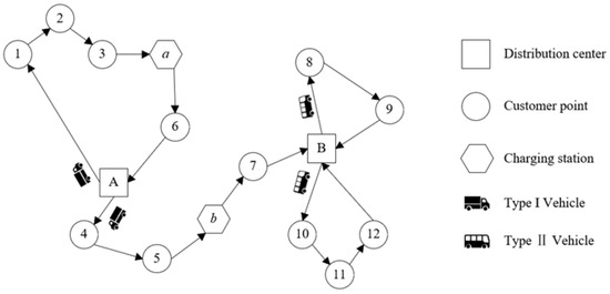
Figure 1.
Description of delivery route. The numerical and alphabetical notations represent the identifiers for customer points and distribution centers, respectively.
3. Model Construction
3.1. Symbol Description
The model symbol description is shown in Table 1.

Table 1.
Symbol description.
3.2. Electric Vehicle Discharge Function
In urban road networks, electric vehicle (EV) distribution is influenced by multiple factors, including vehicle load, driving speed, air resistance, frontal area, and rolling resistance. To ensure that the constructed model aligns more closely with real-world conditions, a nonlinear EV discharge function is formulated [28,29]. The mechanical power of the r-type EV is expressed in Equation (1):
During travel, the discharge function of EV needs to consider the discharge efficiency of the battery and the efficiency of the electric engine to avoid ignoring the loss of electric energy due to the EV engine [30]. The electric vehicle power consumption is the product of the electric vehicle mechanical power and the travel time, and the electric consumption function of the r-type vehicle is shown in Equation (2):
3.3. EV Partial Charging Model
The partial charging strategy involves charging the electric vehicle (EV) based on the subsequent driving distance and the power required for the delivery task, rather than the remaining battery power. Compared to the full charging strategy, the partial charging strategy effectively addresses issues such as low power utilization efficiency and prolonged charging times. The partial charging model proposed in this study is as follows:
Equation (3) represents the total power consumption required for the vehicle to complete delivery services to the remaining customer points after charging. Equation (4) specifies the amount of charging required for the vehicle under different scenarios. Equation (5) defines the charging time for the vehicle, while Equations (6) and (7) establish the node constraints for the vehicle. Here, h denotes the first node visited by vehicle k after leaving the charging station, and u represents the remaining nodes that vehicle kk needs to visit after departing from the charging station.
3.4. Vehicle Travel Time Calculation
Considering the time-dependent characteristics of urban distribution networks, this study proposes a novel vehicle travel time calculation model that accounts for time-varying vehicle speeds. The working time is evenly divided into f time periods. T0 indicates the earliest working moment of the vehicle, and indicates the time node of f time periods. For vehicles in different time periods traveling at different speeds, set the kth r-vehicle in different time periods of the average speed of the vehicle’s driving (p = 1,2,3,…, f − 1), then the vehicle in the time period, (p = 0,1,2,… f − 1) within the travel time as shown in Equation (8):
3.5. Objective Function
1. The distribution center incurs a fixed cost for each vehicle dispatched, which is formulated as:
2. The travel cost of a vehicle is calculated as the product of the sum of the vehicle’s unit time usage cost and the driver’s service cost multiplied by the total time, which includes travel time, unloading time, waiting time, and charging time. This is expressed as:
3. The electricity consumption cost is the total amount of energy consumed by the vehicle during transit, and its formulation is:
4. If the vehicle fails to deliver within the customer’s preferred time window, a waiting cost or penalty cost is incurred, which is expressed as:
3.6. Constraints
Based on Section 3.1, Section 3.2, Section 3.3, Section 3.4 and Section 3.5, the constraints of the model proposed in this paper are as follows:
1. EV capacity constraints:
Equation (13) indicates that the demand of a customer point must not exceed the maximum capacity of the vehicle; Equation (14) ensures that the actual load of the vehicle does not surpass its maximum capacity; Equation (15) describes the relationship between the actual load of the vehicle before and after servicing a customer point; and Equation (16) specifies that the maximum capacity of the vehicle must satisfy the demand of the customer points.
2. Electric vehicle path constraint:
Equation (17) denotes that each customer point is served by one and only one vehicle; Equation (18) denotes that the vehicles depart from the distribution center and each vehicle serves only one path; Equation (19) denotes that the vehicle can return to any distribution center in close proximity after completing the distribution task; Equation (20) restricts the vehicle from going directly from one distribution center to another distribution center; Equation (21) restricts the vehicle from going directly from one charging station to another charging station; and Equation (22) represents the elimination of sub-circuits on the path.
3. Electric vehicle power constraint:
Equation (23) specifies that the electric vehicle (EV) is fully charged upon departure from the distribution center. Equation (24) describes the power relationship between nodes. Equation (25) quantifies the power consumption of the EV on the road segment (i, j). Equation (26) defines the in-transit power constraints for the EV, while Equation (27) outlines the charging constraints. Equation (28) ensures that the EV does not consume any power during the service process. Equation (29) establishes the electric power constraints for the vehicle when passing through each node in the distribution path.
When the range anxiety coefficient is set to 0, it indicates that the vehicle prioritizes the delivery task and only seeks to recharge when the battery is nearly depleted. Conversely, when the range anxiety coefficient is assigned a non-zero value, it reflects the driver’s anxiety during the journey, prompting the driver to halt the distribution task and proceed to the nearest charging station for recharging once the battery level falls below the specified threshold.
4. EV driving time and decision variable constraints:
Equation (30) represents the continuity of the temporal relationship when the vehicle leaves the node; Equation (31) represents the temporal relationship between the previous node and the subsequent node when the vehicle arrives at the node; and Equations (32)–(34) represent the decision variable constraints.
4. Algorithm Design
This paper proposes a multi-center and multi-type electric vehicle routing problem with a time-varying road network as an extension of the electric vehicle routing problem. The adaptive large neighborhood search (ALNS) algorithm, introduced by Ropke and Pisinger [31] in 2006, has demonstrated superior performance in solving vehicle routing problems (VRPs) and has been successfully applied to various VRP variants. However, the ALNS algorithm has certain limitations. During the search process, it may converge to local optima, and its solution efficiency and quality can be compromised if the operators are inefficient. To address these limitations, an improved adaptive large neighborhood search (IALNS) algorithm is designed to solve the multi-center time-dependent electric vehicle routing problem with time windows (MCTEVRPTW).
In the IALNS algorithm, more efficient operators are designed to expand the solution search space. Based on the problem characteristics, damage and repair operators specific to vehicle paths are constructed. An adaptive strategy is introduced to select efficient operators dynamically, and a simulated annealing-based solution acceptance criterion is incorporated to allow for the acceptance of inferior solutions within a certain probability, thereby avoiding convergence to local optima. The fundamental framework of the algorithm and its improvement scheme are outlined as follows.
4.1. Basic Components of ALNS
4.1.1. Probability of Accepting a New Solution Based on Simulated Annealing Algorithm
During the iterative optimization search process, if the newly generated solution outperforms the current solution, it is adopted immediately. Otherwise, the new solution is accepted with a certain probability. The acceptance probability formulae for the new solution proposed in this study are presented in Equations (35) and (36):
In Equations (35) and (36), denotes the value of the objective function of the new solution; denotes the value of the objective function of the current solution; and T denotes the value of the current temperature. The formula for the temperature is: , where a is the cooling rate of the simulated annealing temperature. The initial value of a is set to , where is the rate, assuming that , i.e., in the initial stage, there is a probability of 0.5 to be accepted when the new solution obtained is inferior to the initial solution. After iterations of the algorithm, the temperature will decrease by multiplying it with a constant simulated annealing cooling rate a, and thus the probability of accepting a new solution inferior to the initial one decreases to ensure the convergence of the solution.
4.1.2. Adaptive Strategy
An adaptive strategy is introduced to ensure that the weights of each operator are updated to the optimal state in each iteration loop. In the IALNS algorithm, the weights of each destruction and repair operator are denoted . Higher weights indicate better performance in the last iteration and an increased probability of being selected in the next iteration. In each iteration, the weights are updated according to . The weight update formula is shown in Equation (37):
where is the weight adjustment speed factor and , is the score obtained by operator i in the previous iteration, and is the number of times operator i was used in the previous iteration. The operator weights are then normalized on the basis of classification. During the iteration process, the selection of destruction and repair operators follows the roulette rule.
4.1.3. Algorithm Scoring Strategies
In terms of adaptive large neighborhood search algorithms, there is a lack of research on improving the scoring strategy. Traditional studies generally adopt fixed values, such as = 30, = 20, = 10, etc. In this paper, we propose a randomized scoring mechanism, in which , , and are set as random numbers in the intervals of [27, 33], [17, 23], and [7, 13], respectively. This randomized scoring mechanism aims to enhance the global search capability to increase the probability of the algorithm jumping out of the local optimal solution.
4.2. SOM Initialization
The k-means clustering algorithm is employed to initially group the nodes, and the self-organizing mapping (SOM) method is utilized to initialize the paths of the electric vehicles (EVs). This approach provides a reasonable initial solution for the proposed model, enabling the subsequent optimization algorithm to converge more efficiently toward the global optimal solution. The execution algorithm is outlined in Algorithm 1, with the following steps.
Step 1: At the beginning of the function, declare the global variable P, which contains parameters and data relevant to path planning, such as node coordinates, time windows, and the number of routes.
Step 2: Apply the k-means clustering algorithm to group the node coordinates and output the cluster labels and cluster centers for each node.
Step 3: Traverse each cluster and extract the node indices and time window information associated with that cluster. Sort the nodes according to their time windows, construct a new path, and append the end node to the path.
Step 4: Calculate the path information for each route, including distance, time, and cost metrics, and store the results in a pending collection.
Step 5: Refine and optimize the generated path information to ensure the rationality and feasibility of the paths, thereby providing effective initial solutions for subsequent optimization algorithms.
| Algorithm 1: SOM initialization |
| function kmeans_initial () global P [val, C] = kmeans (P.cor (2:P.node_N (1) +P. node_N (2),:), P. line_N, “Replicates,” 10) task = [] for n from 1 to P. line_N do rn = [1; find (val == n) + 1] tl = P.t_window (rn, 2) tl (1) = 0; tl(end) = 0 [~, ind] = sort(tl) route = [rn(ind)’ − 1, 0] if n == 1 then task = cal_one(route) else task(n) = cal_one(route) end if end for task = Amend(task) end function |
4.3. Destruction Operator Design
4.3.1. Greedy Destruction Operator
The greedy destruction operator evaluates the impact of node removal on path performance by disrupting the existing path structure, thereby selecting the optimal deletion operation. The execution algorithm is detailed in Algorithm 2, with the following steps.
Step 1: Extract the input task information and record the current path along with its associated metrics.
Step 2: Randomly determine the number of nodes to be removed, ranging from 1 to 5, to introduce randomness and uncertainty into the process.
Step 3: Iterate through each route and each removable node, calculate the path performance after node removal, and record the resulting reduction in path performance.
Step 4: Identify the node whose removal results in the largest reduction in path performance, delete it, update the current route’s path information, and return the modified task information.
| Algorithm 2: Greedy destruction operator |
| function destroy_greedy(task) global P task = task. task task1 = task linen = length(task) destroy_n = random_integer (1, 5) node = [] for nn from 1 to destroy_n do df = [] for n from 1 to linen do for j from 2 to task1(n). len − 1 do route_n = task1(n). route route_n(j) = remove(route_n(j)) ret = cal_one(route_n) dfj = task1(n). fit − ret.fit df. append ([n, j, dfj]) end for end for [~, ind] = max (df [:, end]) n = df (ind, 1) j = df (ind, 2) route_n = task1(n). route node. append(route_n(j)) route_n(j) = remove(route_n(j)) task1(n) = cal_one(route_n) end for return task1 end function |
4.3.2. Random Destruction Operator
The random destruction operator optimizes path planning for electric vehicles (EVs) by randomly removing nodes. The core concept of this operator is to assess the impact of node removal on path performance by randomly selecting and deleting nodes from existing paths. The execution algorithm is outlined in Algorithm 3, with the following steps.
Step 1: Extract the input task information and record the current path along with its associated performance metrics.
Step 2: Randomly determine the number of nodes to remove, denoted destroy_n, with a range of 1 to 5.
Step 3: Randomly select a route that contains a sufficient number of demand points, and then randomly choose a valid node position kk for the removal operation.
Step 4: Record the node to be deleted, remove it from the current route’s path, and calculate the performance of the updated path.
| Algorithm 3: Random destruction operator |
| function destroy_random(task) global P task = task. task task1 = task lineN = length(task) destroy_n = random_integer (1, 5) node = [] for nn from 1 to destroy_n do while true do n = random_permute (linen, 1) route = task1(n). route if task1(n). len > 2 then break end if end while k = random_permute(task1(n). len − 2, 1) + 1 node. append(route(k)) route(k) = remove(route(k)) task1(n) = cal_one(route) end for return task1 end function |
4.3.3. Vehicle Path Destruction Operator
The vehicle path destruction operator optimizes the electric vehicle (EV) path by randomly removing all intermediate nodes within a selected path. This operator evaluates the impact of node removal on path performance by disrupting the existing path structure. The execution algorithm is detailed in Algorithm 4, with the following steps.
Step 1: Extract the input task information and record the current path along with its associated performance metrics.
Step 2: Randomly select a route n and verify its length len to ensure that it contains at least two nodes (start and end).
Step 3: After identifying a suitable route, record its intermediate nodes, remove these nodes from the current route’s path, calculate the performance of the updated path, and update the current route information.
Step 4: Upon completing the destruction and updating of the path, return the modified task information.
| Algorithm 4: Vehicle path destruction operator |
| function destroy_route(task) global P task = task. task task1 = task linen = length(task) while true do n = random_permute (linen, 1) if task(n). len < 2 then continue end if route = task(n). route node = route (2: end-1) route (2: end-1) = remove (route (2: end-1)) task1(n) = cal_one(route) break end while return task1 end function |
4.4. Repair Operator Design
4.4.1. Greedy Repair Operator
The greedy repair operator selects the insertion position that minimizes the impact on overall path performance by evaluating the effect of inserting each node on the path’s performance. The execution algorithm is outlined in Algorithm 5, with the following steps.
Step 1: Extract the input s_destroy information to record the current path and the removed nodes.
Step 2: Initialize an empty array to store the performance changes of each route at different insertion positions.
Step 3: Iterate through each route and each potential insertion location, calculate the path performance after inserting the nodes, and record the results.
Step 4: Identify the insertion location that results in the smallest increase in path performance, perform the insertion, and update the current route information.
| Algorithm 5: Greedy repair operator |
| function repair_greedy(s_destroy) global P task = s_destroy. task linen = length(task) for node in s_destroy. node do df = [] for n from 1 to linen do for j from 1 to task(n). len − 1 do route_n = insert(task(n). route, j, node) ret = cal_one(route_n) dfj = ret.fit − task(n). fit df. append ([n, j, dfj]) end for end for [~, ind] = min (df[:, end]) n = df (ind, 1 j = df (ind, 2) route_n = insert(task(n). route, j, node) task(n) = cal_one(route_n) end for return task end function |
4.4.2. Random Repair Operator
The stochastic repair operator selects the insertion position that minimizes the impact on the overall path performance by evaluating the impact of the insertion of each node on the path performance or randomly selects the insertion position if the path performance is degraded. Its execution algorithm is shown in Algorithm 6, with the following steps.
Step 1: Extract information from the input s_destroy to record the current path state and deleted nodes.
Step 2: Create empty array df to store the performance change information of each line at different insertion locations.
Step 3: Iterate over each line and its possible insertion locations, and calculate and record the path performance after inserting nodes.
Step 4: Select the insertion location based on the performance variation. If there is a decrease in performance, use the roulette selection method to randomly select the insertion location. Conversely, select the location with the smallest increase in performance for node insertion and update the line information.
| Algorithm 6: Random repair operator |
| function repair_random(s_destroy) global P task = s_destroy. task linen = length(task) for node in s_destroy. node do df = [] for n from 1 to linen do for j from 1 to task(n). len − 1 do route_n = insert(task(n). route, j, node) ret = cal_one(route_n) dfj = ret.fit − task(n). fit df. append ([n, j, dfj]) end for end for df1 = df (df[:, 3] < 0,:) if not empty(df1) then val = -df1[:, 3] ind = roulette_choose(val) n = df1(ind, 1) j = df1(ind, 2) else [~, ind] = min (df[:, 3]) n = df (ind, 1 j = df (ind, 2) end if route_n = insert(task(n). route, j, node) task(n) = cal_one(route_n) end for return task end function |
4.4.3. Vehicle Path Repair Operator
The vehicle path repair operator optimizes the EV delivery path by locally adjusting the existing path. Its execution algorithm is shown in Algorithm 7, with the following steps.
Step 1: Extract information from the current path solution and set parameters for repair.
Step 2: Randomly select the nodes or path segments to be repaired.
Step 3: Operate on the selected nodes or path segments to generate multiple neighborhood solutions.
Step 4: Evaluate each generated neighborhood solution, calculate its performance index, and select the neighborhood solution with the best performance as the new current solution.
Step 5: Update the selected neighborhood solution to the current path and record the information during the repair process.
| Algorithm 7: Vehicle path repair operator |
| function repair_route(current_solution) global P for iteration from 1 to max_iterations do node_to_repair = random_select_node(current_solution) neighborhood_solutions = [] for operation in [insert, delete, swap] do new_solution = apply_operation (current_solution, node_to_repair, operation) neighborhood_solutions. append(new_solution) end for best_neighbor = null best_improvement = ∞ for solution in neighborhood_solutions do improvement = evaluate(solution)—evaluate(current_solution) if improvement < best_improvement then best_improvement = improvement best_neighbor = solution end if end for if best_neighbor is not null then current_solution = best_neighbor if evaluate(current_solution) < evaluate(best_solution) then best_solution = current_solution end if end if end for return best_solution end function |
5. Algorithm Comparison Experiment
5.1. Parameter Settings
On the premise of selecting the VRPTW dataset in Solomon (http://vrp.galgos.inf.puc-rio.br/media/com_vrp/instances//Solomon/ accessed on 25 March 2025), the algorithm adds distribution centers, vehicle models, time-varying road networks, and charging stations [32]. The starting time of the distribution center is 6:00, and the end time is 22:00. The time-varying speeds in the process of urban logistics distribution will be generated due to the morning and evening peaks, and the average driving speeds of each vehicle model in each time period are as follows:
Type Ⅰ cars: 07:30–08:30, 17:30–18:30 (20 km/h), 11:30–12:30, 13:30–14:30 (30 km/h), other times (40 km/h);
Type II cars: 07:30–08:30, 17:30–18:30 (25 km/h), 11:30–12:00, 13:30–14:00 (35 km/h), other times (60 km/h).
The program was written on MATLAB 2021a and run on an AMD Ryzen9 6900 HX with Radeon Graphics, 3.30 GHz on a Windows 11 64-bit laptop, with a set population size of 100 and a maximum number of iterations of 500. The main parameters of the model were set as shown in Table 2.
Table 2.
Main parameters of the model.
5.2. Algorithm Comparison Experiments for Different Sizes of Customer Points
In order to verify the effectiveness of the proposed algorithm, the IALNS algorithm is compared with the traditional adaptive large neighborhood search (ALNS). The algorithms are selected from the algorithm library proposed by Solomon, and the C-type (aggregated distribution), R-type (random distribution), and RC-type (random aggregated distribution) algorithms are selected and adapted to the research problem of this paper. Three groups of each type of arithmetic are selected to generate the research arithmetic for the problem posed in this paper. In terms of the size of the arithmetic examples, the examples with 25, 50, and 100 customer points are included. The number of inner loops of each algorithm is 20, the optimal solution is taken, the population size is set to 100, the maximum number of iterations is 500, and the maximum running time is 3600 s. The parameter values are the same as in Table 2, and the experimental comparison results are shown in Table 3, where denotes the arithmetic example with customer point size x, TC denotes the optimal solution of the algorithm (CNY), t denotes the running time of the algorithm (s), and Ins denotes the improvement (%).
Table 3.
Algorithm comparison experiments under different scale examples.
As can be seen from Table 3, compared with the ALNS algorithm, the average improvement of the IALNS algorithm proposed in this paper is 6.02% in terms of solution quality, and compared with the ALNS algorithm, the average improvement of the IALNS algorithm proposed in this paper is 9.19% in terms of solution efficiency. Among the 27 test cases proposed in this paper, 21 test cases have better solution quality and solution efficiency than the ALNS algorithm, from which it can be seen that the IALNS algorithm has more obvious advantages in solution efficiency and solution quality. In addition, the running time of the algorithm is slightly longer when the size of customer points is 100, but the vehicle path optimization problem proposed in this paper does not consider real-time factors such as emergencies and does not require high timeliness, so the running time of 500.723 s is acceptable.
6. Sensitivity Analysis
6.1. Simulation Experiment
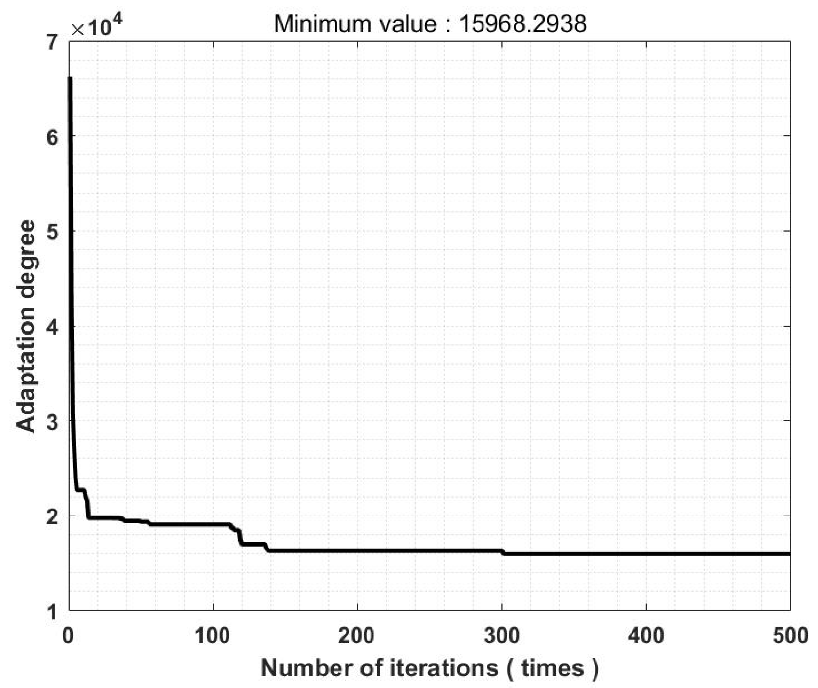
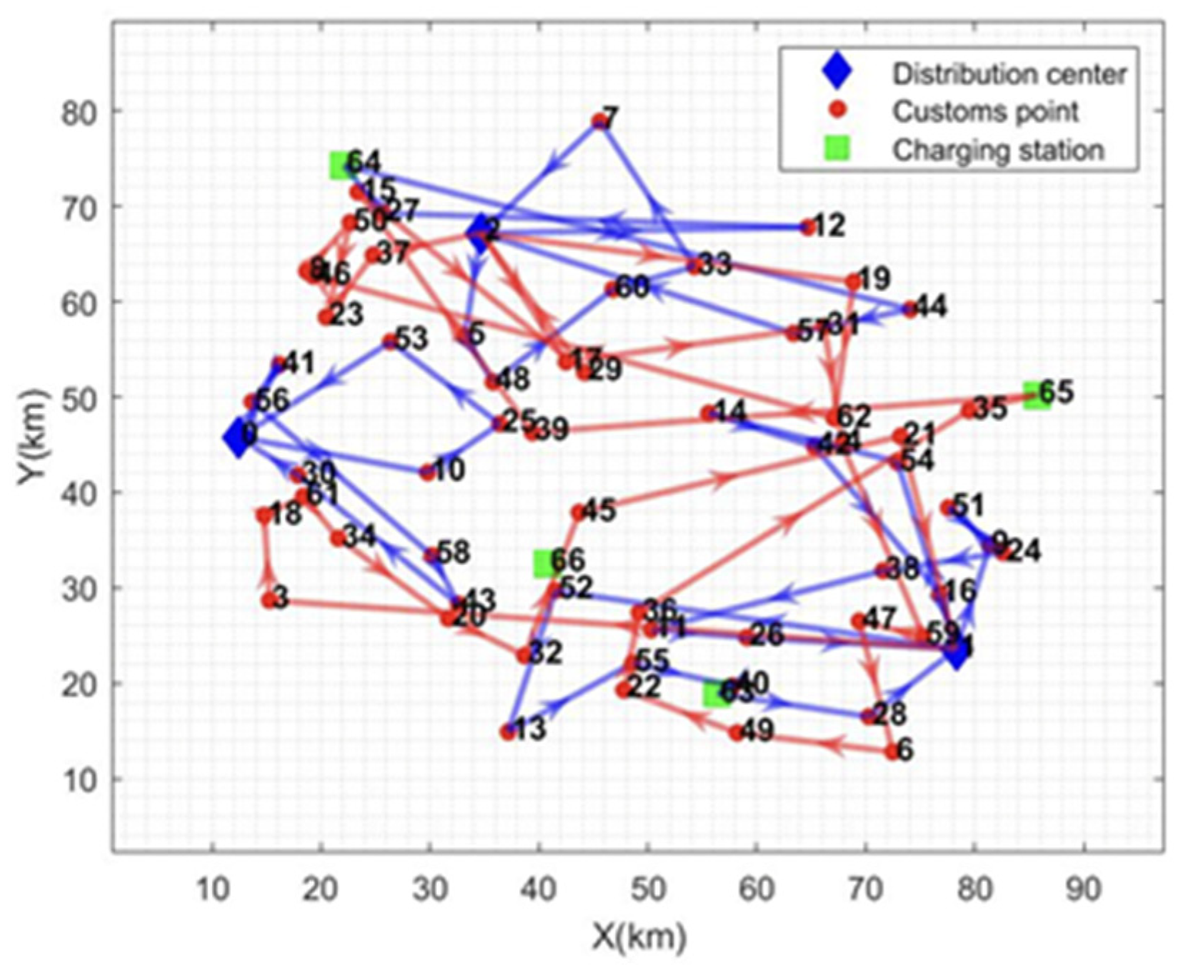
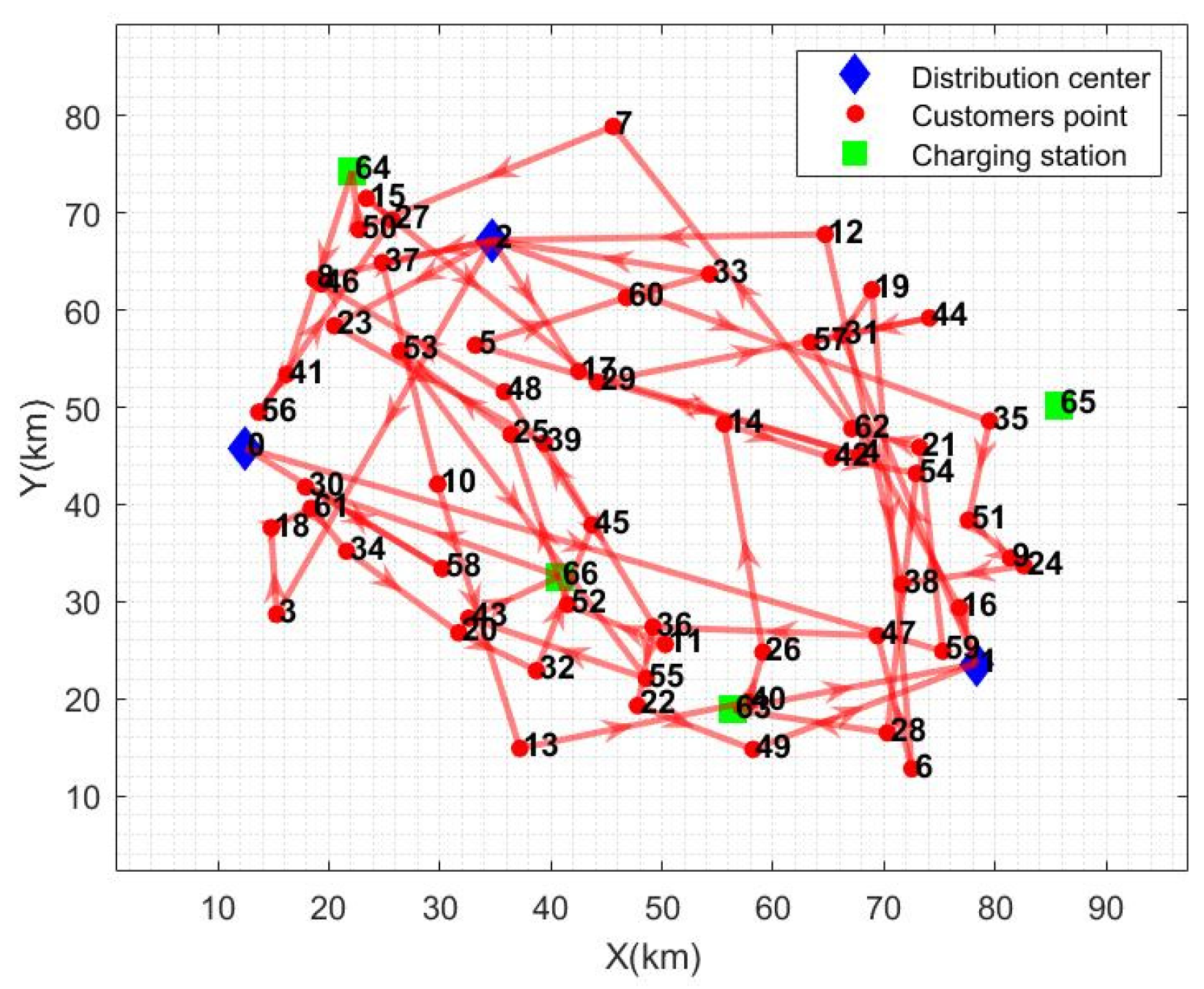
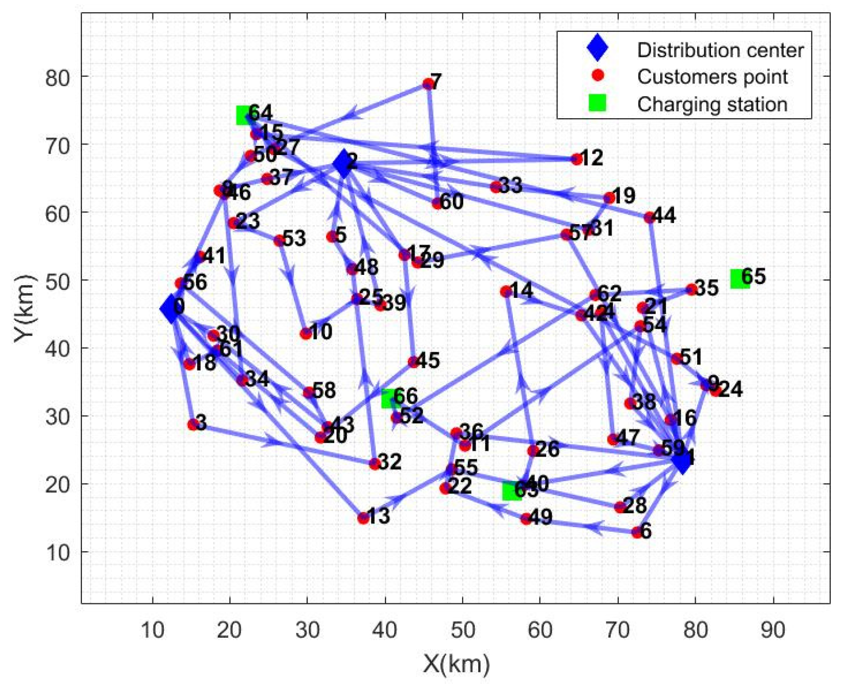
Simulation experiments are carried out using actual data, which comes from 60 order datasets of a fresh food supermarket in X city, including customer point, charging station, distribution center location; customer point demand, and customer point demand time window. Set the population size to 100 and the maximum number of iterations to 500. The parameter values are the same as in Table 2. For 20 cycles within the program, take the optimal solution among them. The specific optimization results are shown in Table 4 and Table 5, the optimal path is shown in Figure 2, the red line in the figure is model I, and the blue line is model II. The iteration curve is shown in Figure 3.
Table 4.
Vehicle routing optimization results.
Table 5.
Cost of each part.
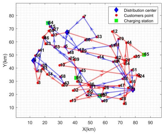
Figure 2.
Optimal path graph.

Figure 3.
Iteration curve.
6.2. Distribution Mode Sensitivity Analysis
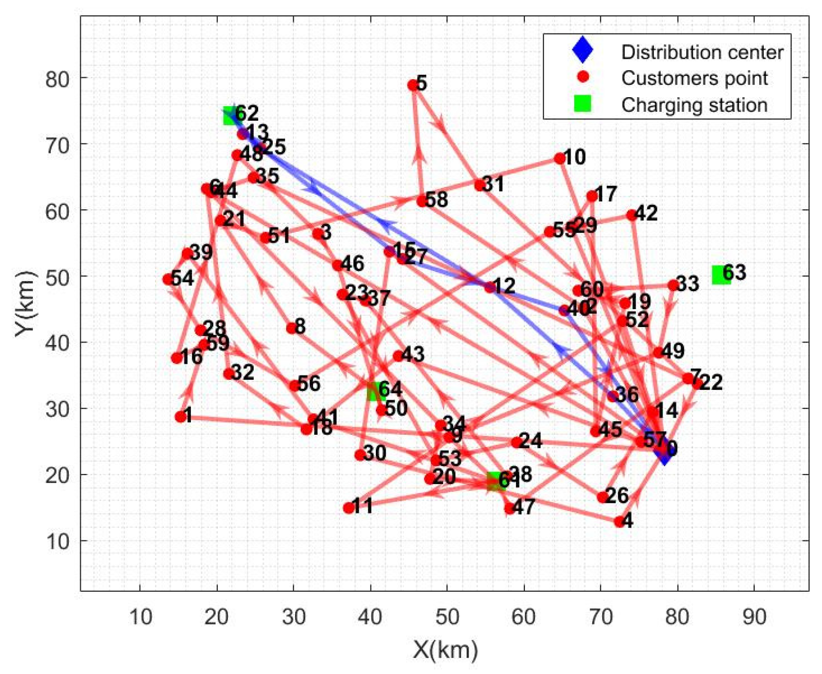
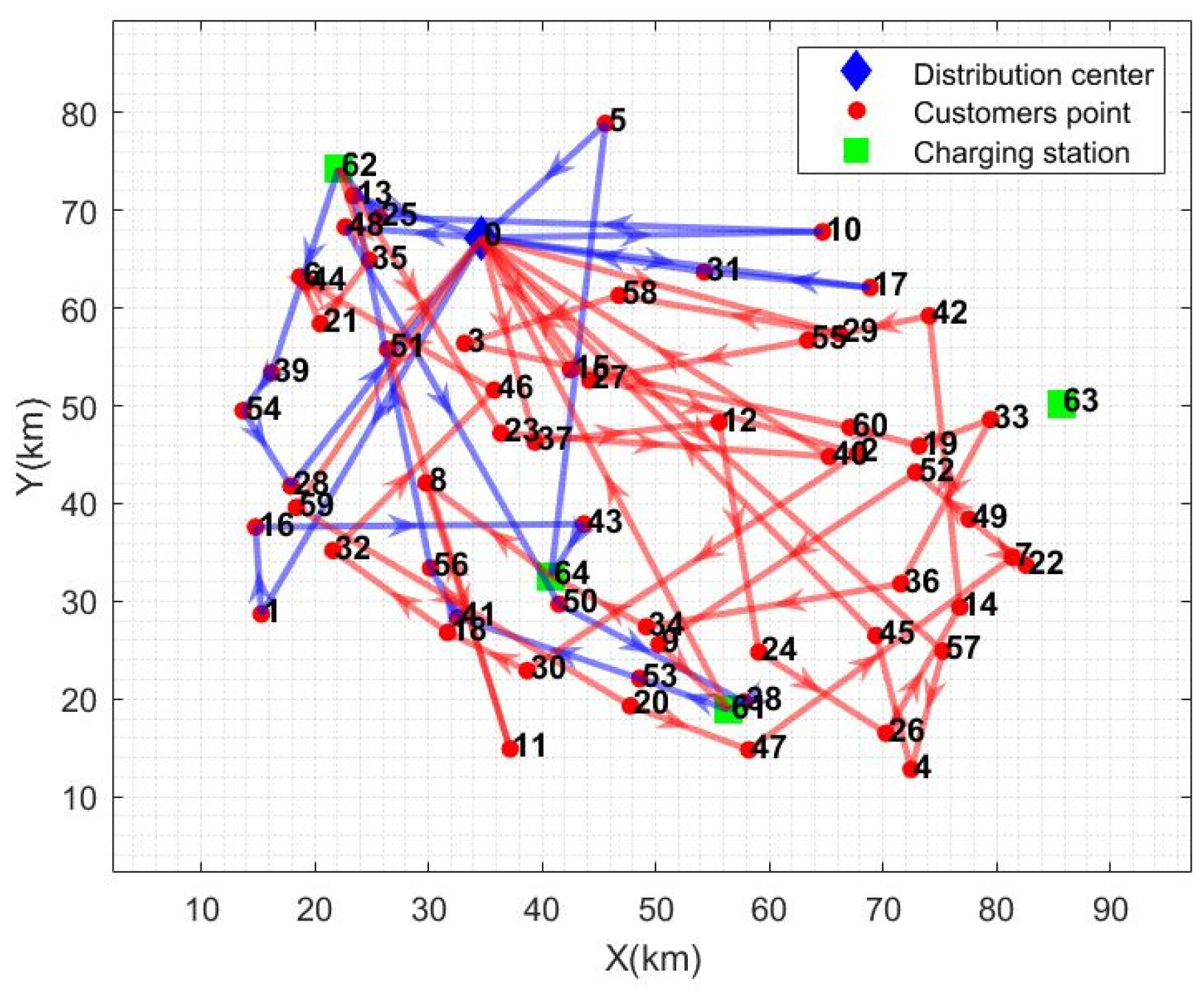
In order to further explore the impact of different distribution modes on the total cost of distribution, path length, power consumption, and distribution time, this paper considers five distribution modes in the study of the multi-model EV vehicle path problem: semi-open multi-distribution centers, closed multi-distribution centers, single distribution centers (no. 0), single distribution centers (no. 1), and single distribution centers (no. 2). Table 6 lists the values of the indicators in different distribution modes, and the values of the parameters are the same as in Table 2. Figure 4, Figure 5, Figure 6 and Figure 7 list the path diagrams of the distribution modes. Among these, TC denotes the total distribution cost (CNY), TD denotes the path length (kilometers), TE denotes the electric energy consumption (kWh), TT denotes the distribution time (minutes), and Ins denotes the improvement (%).
Table 6.
Sensitivity analysis under different distribution modes.

Figure 4.
Closed-path graph of multi-distribution center.
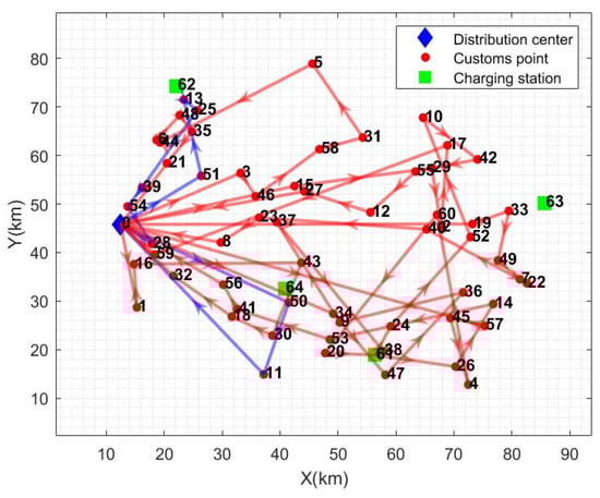
Figure 5.
Single distribution center path graph (no. 0 distribution center).

Figure 6.
Single distribution center path graph (no. 1 distribution center).

Figure 7.
Single distribution center path graph (no. 2 distribution center).
From the calculation results in Table 6, it can be seen that the total cost of distribution has been reduced by an average of 20.44% and the distance of distribution has been reduced by an average of 32.19% compared to the other distribution modes. Electricity consumption is reduced by 18.95% on average, and total distribution time is reduced by 52.53% on average. The path diagrams under the other three distribution modes are given in Figure 5, Figure 6 and Figure 7. As can be seen in Figure 5, the multi-center closed distribution mode requires that the vehicle must return to the original distribution center and the vehicle frequently travels back and forth to the same distribution center, which increases the total cost of distribution, the distribution distance, the electric energy consumption, and the total time of distribution. In Figure 5, when the vehicle completes the delivery of customer point 5, it is closest to distribution center 2; however, the vehicle goes to charging station 64 to recharge and then returns to distribution center 1, which is the furthest distance away. In addition, under the single distribution center model, it is difficult to cover a wide range of customer areas, especially when the distribution of customer points in Figure 6 and Figure 7 is more dispersed, which leads to inefficiency in distribution and increased costs. Moreover, under the single distribution center model, all vehicles must depart from and return to the same location, which lacks the ability of flexible scheduling of vehicles between different distribution centers in the multi-distribution center semi-open model, limiting the optimal allocation of resources. Therefore, the application of the multi-distribution center semi-open distribution model can significantly shorten the vehicle travel distance and travel time, and reduce power consumption and distribution costs.
6.3. Sensitivity Analysis of Fleet Configuration
In order to assess the impact of fleet configuration on the path planning results and to reveal the impact of the indicators on each distribution cost, the fleet configuration is changed for sensitivity analysis, and the fleet configuration contains a type I vehicle fleet, type II vehicle fleet, and a mixed fleet. Table 7 lists the various distribution costs under different fleet configurations, where C1 indicates the fixed cost of vehicles (CNY), C2 indicates the cost of driving (CNY), C3 indicates the cost of electricity (CNY), C4 indicates the cost of the time window penalty (CNY), n indicates the number of vehicles dispatched, and Ins. indicates the magnitude of improvement in the total cost of distribution (%). The parameter values are the same as in Table 2. The path diagram of the type I car is shown in Figure 8, and the path diagram of the type II car is shown in Figure 9.
Table 7.
Sensitivity analysis under different fleet configurations.
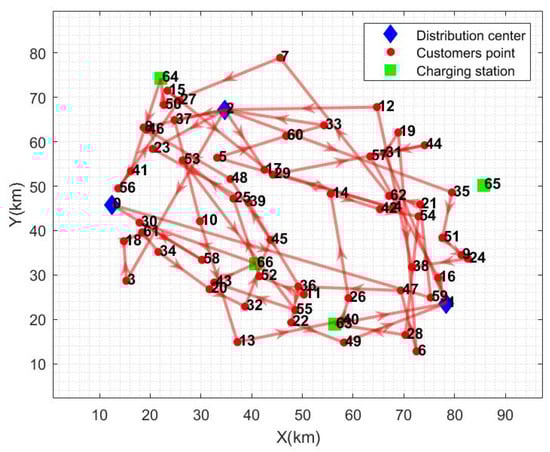
Figure 8.
Type I car path graph.

Figure 9.
Type Ⅱ car path graph.
As can be seen in Table 7, the total distribution cost under the heterogeneous fleet is lower than that under the homogeneous fleet configuration, which indicates that the use of mixed fleet vehicles for distribution under the semi-open distribution model with multiple distribution centers is able to rationally utilize the vehicle resources and thus reduce the total distribution cost. When comparing the costs, although the heterogeneous fleet does not show the optimal value in every cost aspect, in general, the heterogeneous fleet has a better ability to reduce the total distribution cost, which may be attributed to its more flexible combination of vehicle types and route planning methods, which can better adapt to the complex distribution needs and environment. In addition, in terms of fleet selection, compared to Type II vehicles, Type I vehicles have lower charging costs, but higher penalty costs, which means that when the distribution scale is small, choosing faster Type II vehicles can reduce distribution delays and increase customer satisfaction; however, in the case of large-scale distributions and fewer charging stations, it is more economical to choose Type I vehicles with longer range.
6.4. Sensitivity Analysis of Charging Strategy
In order to verify the effectiveness of the partial charging strategy model constructed in this paper, a sensitivity analysis is performed with the model using the full charging strategy. Simulation experiments are carried out using the data in Table 2 and the arithmetic examples in 5.1, and the experimental results are shown in Table 8, where n is the number of vehicles dispatched, CR is the charging rate (%), CT is the charging duration (min), TC is the total cost of distribution (CNY), TE is the electric energy consumption (kWh), and TT is the total duration of distribution (km).
Table 8.
Sensitivity analysis under different charging strategies.
As shown in Table 8, the number of vehicles using both charging strategies is the same. The charging time using the partial charging strategy is 114.63 min, the total cost of distribution is CNY 15,968.2938, the electric energy consumption is 305.8768 kWh, and the total driving time is 1856.172 min. The charging time using the full charging strategy is 157.5 min, the total cost of distribution is CNY 17,278.7114, the electric energy consumption is 375.2441 kWh, and the total driving time is 2751.822 min. Compared with the full charging strategy, the use of the partial charging strategy reduces the charging time by 37.4%, the total distribution cost by 8.21%, the electric energy consumption by 22.68%, and the total distribution time by 48.25%, which indicates that the model of partial charging constructed in this paper can significantly reduce the distribution time, charging time, electric energy consumption, and the total cost of distribution, and proves the effectiveness of the partial charging strategy.
7. Conclusions
In this paper, for the problem of time-dependent multi-distribution center heterogeneous fleet path optimization and charging strategy selection, an improved adaptive large neighborhood search algorithm is used to solve the problem. Simulation experiments are conducted using standard test cases and real cases, and the following conclusions are drawn.
1. In terms of algorithm design, the improved adaptive large neighborhood search algorithm proposed in this paper uses a new operator scoring strategy and a new solution acceptance criterion. According to the actual problem, efficient vehicle path destruction and repair operators are designed to expand the search space of the solution, effectively preventing the algorithm from falling into local optima and further improving the solution efficiency and solution quality. In addition, an adaptive strategy is introduced to ensure that the weights of each operator are updated to the optimal state in each iteration loop.
2. In terms of model construction, this study introduces several key innovations. First, a nonlinear power consumption measurement model is proposed, which comprehensively considers the effects of actual vehicle load, travel speed, vehicle parameters, and road impedance on energy consumption. This model enables a more accurate calculation of the vehicle’s power consumption during distribution services. Second, the implementation of a partial charging strategy effectively reduces the total distribution time, energy consumption, and overall distribution costs. Third, compared to traditional homogeneous fleets, the adoption of a heterogeneous fleet not only lowers the total distribution costs but also achieves an effective balance between economic and environmental benefits. Finally, in contrast to other distribution models, the multi-center semi-open distribution model significantly shortens the distribution distance and time, reduces electric energy consumption, and provides a practical foundation for the sustainable development of green logistics.
3. In terms of managerial implications for logistics enterprises, this study demonstrates significant value. First, by optimizing distribution routes and charging strategies, it substantially reduces operational costs. Through the rational scheduling of electric vehicles (EVs) and fuel-powered vehicles, vehicle load rates are increased, thereby lowering electricity and maintenance expenses. Second, the study enhances distribution efficiency and service quality. Time-dependent route optimization enables real-time responses to traffic conditions and customer demand fluctuations, ensuring timely completion of delivery tasks and improving customer satisfaction. Additionally, the flexible scheduling of heterogeneous fleets and the semi-open distribution model expand the scope of distribution, strengthening the enterprise’s market competitiveness.
4. From the perspective of environmental sustainability, the integration of EVs into logistics distribution significantly reduces carbon emissions and energy consumption. This allows logistics enterprises to better fulfill their social responsibilities and enhance their brand image. Furthermore, the optimization of charging strategies, such as the partial charging strategy proposed in this study, extends battery lifespan and reduces battery replacement costs, thereby minimizing resource waste. Finally, this research provides logistics enterprises with scientific management tools and decision-making support. By incorporating advanced optimization algorithms and data analysis techniques, enterprises can achieve intelligent management of the distribution process, improve resource utilization efficiency, and lay the foundation for future business expansion and technological upgrades.
In summary, this paper provides a feasible solution for the time-dependent electric vehicle routing problem with a multi-depot semi-open heterogeneous fleet, demonstrating significant adaptability and robustness, particularly in addressing heterogeneous fleets and distribution modes. However, this study has certain limitations. Future research could introduce more complex real-world scenarios and diverse uncertainty factors to further expand the model’s applicability and enhance its effectiveness in various logistics environments. For example:
1. The current model includes only two types of vehicles with different capacities/sizes, and future studies could incorporate a wider variety of vehicle types;
2. The waiting time for electric vehicles at charging stations due to queuing is not considered;
3. Uncertainties in customer demand and demand time windows are not addressed.
Such improvements would further enhance the adaptability of the electric vehicle routing problem and increase the practical value of the model in dynamic logistics environments.
Author Contributions
Conceptualization, H.M. and T.W.; methodology, H.M. and T.W.; validation, H.M. and T.W.; formal analysis, H.M. and T.W.; investigation, H.M.; writing—original draft preparation, H.M.; writing—review and editing, T.W.; visualization, H.M.; supervision, T.W. All authors have read and agreed to the published version of the manuscript.
Funding
This work was supported by the National Natural Science Foundation of China, grant No. 71771111.
Data Availability Statement
Data supporting this study are available from the corresponding author upon reasonable request.
Conflicts of Interest
The authors declare no conflicts of interest.
References
- Schneider, M.; Stenger, A.; Goeke, D. The electric vehicle-routing problem with time windows and recharging stations. Transp. Sci. 2014, 48, 500–520. [Google Scholar] [CrossRef]
- Ahmed, Z.; Yousefikhoshbakht, M. A hybrid algorithm for the heterogeneous fixed fleet open vehicle routing problem with time windows. Symmetry 2023, 15, 486. [Google Scholar] [CrossRef]
- Jiang, C.; Zhou, L.; Zheng, J.; Shao, Z. Electric vehicle charging navigation strategy in coupled smart grid and transportation network: A hierarchical reinforcement learning approach. Int. J. Electr. Power Energy Syst. 2024, 157, 109823. [Google Scholar] [CrossRef]
- He, M.; Yang, M.; Fu, W.; Wu, X.; Izui, K. Optimization of Electric Vehicle Routes Considering Multi-Temperature Co-Distribution in Cold Chain Logistics with Soft Time Windows. World Electr. Veh. J. 2024, 15, 80. [Google Scholar] [CrossRef]
- Veena Vani, B.; Kishan, D.; Ahmad, M.W.; Naresh Kumar Reddy, B. Bat Optimization Model for Electric Vehicle Route Optimization Under Time-of-Use Electricity Pricing. Wirel. Pers. Commun. 2023, 131, 1461–1473. [Google Scholar] [CrossRef]
- Wang, H.; Ran, H.; Zhang, S. Location-routing optimization problem of country-township-village three-level green logistics network considering fuel-electric mixed fleets under carbon emission regulation. Comput. Ind. Eng. 2024, 194, 110343. [Google Scholar] [CrossRef]
- Afsane, A.; Hossein, Z.; Hassanzadeh, S.A. Routing a mixed fleet of conventional and electric vehicles for urban delivery problems: Considering different charging technologies and battery swapping. Int. J. Syst.Sci. Oper. Logist. 2023, 10, 2191804. [Google Scholar]
- Wang, R.; Zhang, F.; Ding, L.; Jiang, J.; Han, Z. A Novel Approach for Optimizing Mixed Hazardous Material Fleet Vehicle Routing Problem Method Through Intermediate Bulk Container Sharing with Adaptive Intuitionistic Fuzzy Large Neighborhood Search. Int. J. Fuzzy Syst. 2024, 1–19. [Google Scholar] [CrossRef]
- Sarbijan, M.; Behnamian, J. Multi-fleet feeder vehicle routing problem using hybrid metaheuristic. Comput. Oper. Res. 2022, 141, 105696. [Google Scholar] [CrossRef]
- Sun, H.; He, M.; Gai, Y.; Cao, J. Optimization of fresh food logistics routes for heterogeneous fleets in segmented transshipment mode. Mathematics 2024, 12, 3831. [Google Scholar] [CrossRef]
- Nistha, D.; Ajinkya, T. A multi-depot vehicle routing problem with time windows, split pickup and split delivery for surplus food recovery and redistribution. Expert Syst. Appl. 2023, 232, 120807. [Google Scholar]
- Alaia, E.B.; Dridi, I.H.; Bouchriha, H.; Borne, P. Genetic Algorithm for Multi-Criteria Optimization of Multi-Depots Pick-up and Delivery Problems with Time Windows and Multi-Vehicles. Acta Polytech. Hung. 2015, 12, 155–174. [Google Scholar]
- Nunes, S.; Freitas, J.; Ricardo, S. A variable neighborhood search-based algorithm with adaptive local search for the Vehicle Routing Problem with Time Windows and multi-depots aiming for vehicle fleet reduction. Comput. Oper. Res. 2023, 149, 106016. [Google Scholar]
- Li, J.; Wang, R.; Li, T.; Lu, Z.; Pardalos, P.M. Benefit analysis of shared depot resources for multi-depot vehicle routing problem with fuel consumption. Transp. Res. Part D 2018, 59, 417–432. [Google Scholar]
- Ruiz, E.; Soto-Mendoza, V.; Barbosa, A.E.R.; Reyes, R. Solving the open vehicle routing problem with capacity and distance constraints with a biased random key genetic algorithm. Comput. Ind. Eng. 2019, 133, 207–219. [Google Scholar] [CrossRef]
- Ichoua, S.; Gendreau, M.; Potvin, J.Y. Vehicle dispatching with time-dependent travel times. Eur. J. Oper. Res. 2003, 144, 379–396. [Google Scholar]
- Gmira, M.; Gendreau, M.; Lodi, A.; Potvin, J.-Y. Tabu search for the time-dependent vehicle routing problem with time windows on a road network. Eur. J. Oper. Res. 2021, 288, 129–140. [Google Scholar]
- Hesam Sadati, M.; Çatay, B.; Aksen, D. An efficient variable neighborhood search with tabu shaking for a class of multi-depot vehicle routing problems. Comput. Oper. Res. 2021, 133, 105269. [Google Scholar]
- Stoia, S.; Laganà, D.; Ohlmann, W.J. Dynamic pickup-and-delivery for collaborative platforms with time-dependent travel and crowd shipping. Eur. J. Oper. Res. 2025, 322, 70–84. [Google Scholar] [CrossRef]
- Desaulniers, G.; Errico, F.; Irnich, S.; Schneider, M. Exact algorithms for electric vehicle-routing problems with time windows. Oper. Res. 2016, 64, 1388–1405. [Google Scholar]
- Meng, M.; Ma, Y. Route Optimization of Electric Vehicle considering Soft Time Windows and Two Ways of Power Replenishment. Adv. Oper. Res. 2020, 2020, 5612872. [Google Scholar]
- Wang, Z.; Ye, K.; Jiang, M.; Yao, J.; Xiong, N.N.; Yen, G.G. Solving hybrid charging strategy electric vehicle based dynamic routing problem via evolutionary multi-objective optimization. Swarm Evol. Comput. 2022, 68, 100975. [Google Scholar]
- Ying, L.; Flavien, L.; Kenneth, S. The electric on-demand bus routing problem with partial charging and nonlinear function. Transp. Res. Part C 2023, 157, 104368. [Google Scholar]
- Montoya, A.; Guéret, C.; Mendoza, J.E.; Villegas, J.G. The electric vehicle routing problem with nonlinear charging function. Transp. Res. Part B 2017, 103, 87–110. [Google Scholar]
- Yuan, P.; Luo, M.; Miao, G.; Li, J. Problem of patient transport route planning for battery electric vehicles considering a flexible charging strategy. Transp. Res. Rec. J. Transp. Res. Board 2024, 2678, 198–225. [Google Scholar]
- Liu, J.; Yang, X.; Zhuge, C. A joint model of infrastructure planning and smart charging strategies for shared electric vehicles. Green Energy Intell. Transp. 2024, 3, 100168. [Google Scholar]
- Zhang, S.; Zhou, T.; Fang, C.; Yang, S. A novel collaborative electric vehicle routing problem with multiple prioritized time windows and time-dependent hybrid recharging. Expert Syst. Appl. 2024, 244, 122990. [Google Scholar]
- Demir, E.; Bektas, T.; Laporte, G. An adaptive large neighborhood search heuristic for the pollution-routing problem. Eur. J. Oper. Res. 2012, 223, 346–359. [Google Scholar]
- Ma, B.; Hu, D.; Chen, X.; Wang, Y.; Wu, X. The vehicle routing problem with speed optimization for shared autonomous electric vehicles service. Comput. Ind. Eng. 2021, 161, 107614. [Google Scholar] [CrossRef]
- Zhang, S.; Gajpal, Y.; Appadoo, S.; Abdulkader, M. Electric vehicle routing problem with recharging stations for minimizing energy consumption. Int. J. Prod. Econ. 2018, 203, 404–413. [Google Scholar]
- Ropke, S.; Pisinger, D. An adaptive large neighborhood search heuristic for the pickup and delivery problem with time windows. Transp. Sci. 2006, 40, 455–472. [Google Scholar] [CrossRef]
- Solomon, M. Algorithms for the Vehicle Routing and Scheduling Problems with Time Window Constraints. Oper. Res. 1987, 35, 254–265. [Google Scholar] [CrossRef]


Disclaimer/Publisher’s Note: The statements, opinions and data contained in all publications are solely those of the individual author(s) and contributor(s) and not of MDPI and/or the editor(s). MDPI and/or the editor(s) disclaim responsibility for any injury to people or property resulting from any ideas, methods, instructions or products referred to in the content. |
© 2025 by the authors. Licensee MDPI, Basel, Switzerland. This article is an open access article distributed under the terms and conditions of the Creative Commons Attribution (CC BY) license (https://creativecommons.org/licenses/by/4.0/).