Modeling the Relationship Between Radon Anomalies and Seismic Activity Using Artificial Neural Networks and Statistical Methods

Abstract

The paper presents an approach for detecting anomalies in radon concentration in seismically active areas. It involves training multiple artificial neural networks (ANNs) to predict radon concentration during periods without seismic events. The trained ANNs model the typical radon variations under non-seismic conditions, and the predicted values for normal radon behavior are compared with actual radon concentrations around the time of recorded earthquakes. Significant deviations from the predicted values are interpreted as radon anomalies potentially associated with upcoming seismic events. The methodology includes wavelet transformation for noise removal, a multilayer ANN trained using the Levenberg–Marquardt algorithm, and a segmentation approach based on radial zones (annuli) for localized predictions. Large datasets from three radon measurement stations in Bulgaria—Yambol, Dimitrovgrad, and Krupnik—were used. Data from seismic periods were excluded during the training of the neural networks to ensure that the models learn only the natural radon variations under non-seismic conditions. Key results indicate that, in Yambol and Dimitrovgrad, the actual radon concentration exceeds the predicted normal levels during earthquakes, whereas in Krupnik, radon concentration is lower than expected during seismic events. Analysis of the pre-seismic period shows elevated radon levels 48 h before earthquakes at some stations, while expected anomalies were not observed at others. Through this study, we demonstrate the effectiveness of ANN models in modeling radon behavior under non-seismic conditions and identifying deviations that may be linked to seismic activity. We believe that the obtained results contribute to the ongoing discussion on radon concentration anomalies as potential earthquake precursors and suggest that local geological and environmental factors may further influence radon emissions in different ways.

1. Introduction

Earthquakes cause significant damage to people and the environment. Their prediction is the subject of extensive scientific research. Timely warning of the population can enable evacuation and save human lives. People can take measures to protect their property and minimize potential damage. Early notification of civil protection and emergency services provides time for preliminary preparation, better coordination, and more effective response by those involved in these activities. For this reason, many scientists study various phenomena and processes as potential precursors of seismic activity and seek methods for earthquake prediction.

For centuries, unusual animal behavior has been reported before critical events such as earthquakes. Observations include decreased activity among mammals and birds up to three weeks before an earthquake [1], strange animal behavior without vocalizations, and cases of various animals giving birth days to almost a month earlier prior to major earthquakes. Other studies have documented unusual changes in the animal kingdom days and hours before major earthquakes, including anxiety, chaotic movements, or even mass migrations [2,3,4]. Animals are particularly sensitive to physical and chemical changes in the environment. Before an earthquake, electromagnetic anomalies, changes in atmospheric pressure, alterations in groundwater, and other phenomena are observed. Such unexpected changes and anomalies are being investigated and studied as potential precursors to earthquakes.

In [5], geophysical and astronomical factors such as Earth–Moon gravitational forces, their varying distances, and localized gravity fluctuations are utilized to develop machine learning regression models that enhance earthquake predictions. Hypotheses on the relationship between space weather and earthquakes, as well as the potential triggering of seismic activity by strong solar flares, have also been investigated [6]. Other studies indicate a correlation between tides and earthquakes, suggesting that tidal forces could be used as a predictor for potential seismic events [7].

During the development of a seismic process, disturbances in the geomagnetic field are observed. Volvach et al. utilized magnetic field data to identify changes in geophysical fields associated with earthquakes of magnitude greater than 7. They found that the parametric resonance of surface geomagnetic oscillations could be considered a precursor to earthquakes [8].

How the ground shakes and the damage an earthquake can cause depend on the properties of the soil and rocks beneath it. One of the most important indicators of this is the so-called wave velocity (Vs), which shows how quickly seismic waves travel through soil or rock. Comina et al. used a combination of geological modeling and geophysical measurements to create a database of shear wave velocity values for the Piedmont region in Italy [9]. Such information can be used for more accurate predictions of seismic motions in the region; however, specific geological characteristics limit its universal application to other areas. Rău et al. developed a model to study how seismic waves (P and S waves) propagate through Earth’s layers. This enhances the understanding of seismic activity in earthquake-prone zones and helps more accurately determine the location and characteristics of earthquakes [10]. Ji et al. investigated the mechanisms and environment of earthquake swarms by analyzing data on seismic wave propagation through underground layers. They created three-dimensional models of P-wave velocity (waves that propagate first), S-wave velocity (slower but more destructive waves), and the ratio between them (Vp/Vs). These models revealed that, beneath the highly seismically active area of Changdao, there are significant anomalies with high Vp/Vs values reaching depths of up to 30 km [11].

A thorough review of the scientific literature reveals that earthquake prediction is a highly complex process. Researchers have studied a wide variety of potential precursors, including seismic, geodetic, geochemical, geological, atmospheric, geomagnetic, electrical, and others. On the other hand, the unique conditions in each seismic region also play a significant role in how an earthquake develops. These include region-specific characteristics such as soil type, terrain slope, fault structure, and the thickness of sedimentary layers. Human activities, such as construction, changes in urban infrastructure, mining, and the development of water facilities, can also influence the way seismic waves propagate. The specific characteristics of different regions motivate the development of individual mathematical models for earthquake prediction tailored to each specific area. It is not necessary to examine all possible environmental characteristics as predictors. Instead, it is sufficient to identify and analyze the factors that have the strongest correlation with seismic activity in the particular region.

Radon in groundwater and soil is considered one of the most significant geochemical precursors, used to detect chemical and physical changes preceding earthquakes. Stress in the Earth’s crust causes the release of radon, leading to changes in its concentration in soil and groundwater. Therefore, this gas can be a valuable predictor in regions where faults are active and strong earthquakes are anticipated. Radon as a precursor to earthquakes has been specifically studied and utilized for developing a model in our research.

The approach we adopt for this study involves the use of ANNs trained with the Levenberg–Marquardt algorithm, as well as the segmentation of data into multidimensional layers (annuli) to improve the accuracy of predictions. Our choice of ANNs is based on several key characteristics of these structures that are important for our research. ANNs are particularly effective in predicting complex non-linear relationships, such as those between seismic activity and radon concentration. Furthermore, ANNs are capable of adapting to different stations by identifying patterns in the data that are difficult to detect using classical statistical methods. ANNs perform well with large and high-dimensional datasets, which are the focus of our study. One of the most important reasons for choosing ANNs was the noise characteristics in the dataset we worked with. These data were obtained from stationary monitoring stations in three different cities in Bulgaria. The measuring instruments at each of these stations, along with geological and climatic characteristics, as well as random factors, introduce a certain amount of noise into the data. ANNs do not directly memorize the input data; instead, they extract patterns and build representations of them. When the network is properly regularized, it does not “overfit” to the specific noise in the training dataset but rather focuses on the essential features in the data. Additionally, ANNs transform input data through multiple layers and activation functions, which helps smooth out non-systematic variations (noise). The hyperbolic tangent function (tanh) used in our approach acts as a limiting function, reducing the influence of extremely high or low values, which are often artifacts of noise. In the study, we applied an approach in which ANNs operate with different rings (annuli) of the input data, with each ANN being trained in a separate region. This allowed us to create local models that are more accurate for their respective zones and do not become “defocused” by random fluctuations outside their range. This approach reduced the impact of noisy data in different areas by dividing the data processing into independent subspaces. And although we also use wavelet transform for noise removal, the choice of ANNs, along with all their other advantages, further minimized the effect of noise in the data.

For the first time in Bulgaria, we employ a multitude of ANNs to analyze and approximate the typical behavior of radon in the soil at several geolocations across the country. We then compare these data with periods when seismic activity is recorded. This enables us to evaluate the impact of earthquakes on radon concentrations in the respective regions.

To address all these objectives and challenges, we structured the paper in a way that follows the stages of the conducted research. The study’s context (in our case, radon as a predictor), the methodology involving statistical analysis and ANNs, the results, and the discussion are presented sequentially. Thus, Section 2 presents the conventional scientific perspective on radon and its role in earthquake prediction, while Section 3, Section 4 and Section 5 introduce the innovative methods—statistical analyses, neural networks, and the segmentation approach. We believe that this structure clearly distinguishes the traditional from the novel approach in the study and facilitates the reader’s understanding by gradually building comprehension of the research problem and its solution. More specifically, the paper follows this sequence: Section 2 “Radon as an Earthquake Predictor” provides a detailed discussion of radon as a potential earthquake predictor, summarizing previous studies and their significance for seismic forecasting. Section 3 “Statistical Study of the Data Obtained from Radon Stations” describes the statistical methods applied in the study, including preprocessing of the data, exploratory analysis, and key statistical indicators. Section 4 “Use of ANNs in Noisy Data with Large Sample Sizes” focuses on the application of ANNs for modeling radon concentration, particularly in the presence of noise in the data. The methodology for training, validation, and testing of the ANN is described in detail. Section 5 “Model for Predicting Radon Levels through the Construction of Multiple ANNs” presents the predictive model for radon anomalies, addressing segmentation of the input space, wavelet transformation for noise removal, and interpolation techniques used. Section 6 “Experiments” contains the results and discussion, emphasizing key findings and model performance. The paper concludes with Section 7 “Conclusions” which summarizes the main contributions and outlines directions for future research.

2. Radon as an Earthquake Predictor

Traditional methods for analyzing and describing radon concentrations include regression analysis [12,13,14] and the use of time series [15,16,17]. Numerical methods and polynomial approximations are also commonly employed [18,19,20]. Many approaches based on machine learning methods have also gained prominence and are widely used by researchers studying radon levels. Notable works include those presented by [21,22,23], among others. Recently, many authors have focused their attention on the field of artificial intelligence, represented by ANNs. Examples of such works include [24,25,26]. The interest in these artificial intelligence tools is entirely understandable—they are powerful approximation tools, especially when dealing with highly non-linear problems. Considering their adaptive nature and ability to continuously learn, it is clear why they are favored for approximation tasks characterized by strong indeterminacy and stochasticity. Additionally, their excellent compatibility with classical methods further enhances their appeal.

The authors of [27] utilize intelligent algorithms such as ANNs, multiple linear regression (MLR), and decision trees (DT) to detect radon anomalies caused by seismic activity. The dataset is divided into two categories—periods of seismic activity and stable periods—using time intervals of 7 days before and after the earthquake. Data from the stable periods are used for training and cross-validation of the intelligent algorithms. Statistically significant radon anomalies are identified through the difference between simulated and measured radon levels. The authors find that all the algorithms show significant deviations in radon concentration around the time of the earthquake, with the ANN model demonstrating the best performance.

To identify radon anomalies in groundwater, Feng et al. developed three models: the long short-term memory (LSTM) model with auxiliary data, the empirical mode decomposition long short-term memory (EMD-LSTM) model with auxiliary data, and the EMD-LSTM model without auxiliary data. They examined different time windows around earthquakes, including ±10, ±30, ±50, and ±100 days before and after seismic events. The highest prediction accuracy was achieved for the ±30-day period. The EMD-LSTM model demonstrated the best predictive capability, identifying five potential radon anomalies associated with seven earthquakes [28]. The applicability of LSTM models for detecting potential hydrological anomalies preceding earthquakes has also been confirmed in other studies [29].

Investigating the relationship between soil radon levels and seismic activity, Tareena et al. developed three models using a feed-forward neural network (FFNN), recurrent neural network (RNN), and support vector regression (SVR). They utilized data from a fault line and searched for anomalies in radon time series caused by seismic events. To achieve this, they compared actual and calculated radon concentrations while accounting for various meteorological and statistical parameters. Their analyses demonstrated that, with the application of machine learning techniques, anomalies in radon time series caused by earthquakes can be successfully identified, provided the environment is carefully characterized, and noise is excluded. The best results for radon assessment were achieved using FFNN, while SVR performed the weakest [30].

Shepelev et al. utilized machine learning methods to analyze the relationships between changes in radon concentration, seismic activity, and meteorological data. Radon variations are described using temporal, statistical, and complexity features, which are used to train a linear classification method to classify seismic activity as either “strong” or “weak”. Two classification models are investigated, differing in how they classified seismic events as “strong” or “weak”—one based on the magnitude of events and the other on intensity in points. The researchers found that changes in subsurface radon concentration could serve as an implicit precursor to earthquakes [31].

In [32], the interrelationship, interdependence, and connectivity of various factors with earthquakes are examined, including water level, radon gas, animal behavior, hydro-chemical, and dilatancy–diffusion. The authors analyze time series using various machine learning algorithms, including SVM, regression, decision tree, Bayesian model, and ANN models.

Planinić et al. used soil radon data collected over 4 years with LR-115 nuclear track detectors. They studied the influence of meteorological parameters on temporal variations in radon levels while also observing seismic activities. They determined the linear equation of multiple regression, which allows for the reduction of radon variations caused by barometric pressure, rainfall, and air temperature. Based on radon anomalies, the authors identified earthquakes with magnitudes greater than 3 at epicentral distances of less than 200 km [33].

In [34], a study of soil radon concentration in a geological fault zone is presented, with data collected over the course of one year. The ensemble empirical mode decomposition (EEMD) method is used to decompose the signal into its characteristic modes. On the physically significant modes obtained through EEMD, the Hilbert–Huang transform (HHT) is applied to represent the time–energy–frequency profile of the soil radon time series. After removing the periodic components from the time series, the analyses revealed a strong correlation between the recorded radon anomalies and local seismic events.

In another large-scale study covering data from the past 50 years in Greece, soil radon time series are also analyzed. The authors used the method of singular spectrum analysis to identify change points in the radon time series. They eliminated the influence of meteorological parameters and discovered correlations between radon variations and earthquakes with magnitudes ranging from M3.5 to 6.5. The anomalies lasted from days to weeks, depending on the type of fault [35].

A study on the various factors influencing soil radon concentrations is presented in [36]. The authors classify radon anomalies in groundwater, explore their causes, examine the environmental influences, and analyze the effects of soil and rock structures on radon migration. They emphasize the potential of machine learning for classifying and predicting radon anomalies caused by earthquakes, experimenting with boosted trees, support vector machines, neural networks, multivariate linear regression, decision tree algorithms, and others.

A study of radon data from a hot spring spanning a 38-year period is presented in [37]. Using wavelet coherence analysis, the authors identified the factors influencing radon fluctuations, including spring discharge, water temperature, rainfall, and barometric pressure. They developed decision tree models to simulate the “background” radon levels. Anomalies are identified by comparing observed radon changes with the modeled “background” fluctuations. The modeled “background” variations in the radon time series are then compared with observations during seismic activity periods. Using this method, they identified 15 potential radon anomalies among 24 selected earthquakes. The authors found that the detected anomalies were also accompanied by changes in water temperature and spring discharge. They attribute the anomalous increase in radon to its continuous supply from newly formed internal surfaces of cracks to the aquifer system. The anomalous decrease in radon is explained by radon partitioning into the gas phase and changes in the mixing ratio of shallow and deep water.

In [38], a study is presented where the empirical mode decomposition (EMD) method is used to detect oscillations in radon time series. The radon time series are decomposed into various oscillatory modes, known as intrinsic mode functions (IMFs). After applying the Hilbert–Huang transform (HHT) to the significant IMFs, several interesting non-linear characteristics are identified. The temporal variation of the instantaneous energy showed a strong correlation with four local earthquakes during the study period. Most interestingly, interruptions in the temporal evolution of the instantaneous energy function are observed prior to these local earthquakes. Many more studies on radon precursors for earthquake forecasting have been systematically reviewed in [39,40].

Another commonly used approach for modeling uncertainty and dynamically updating predictions based on new data is Bayesian methods. For example, Bayesian dynamic modeling is used for the probabilistic prediction of pavement conditions, integrating multiple uncertain factors—weather conditions, mechanical load, pavement age, and other parameters [41,42,43,44]. This technique enables adaptive real-time model adjustments, improving the accuracy of long-term forecasts. In addition to various scientific and engineering disciplines, Bayesian methods are also applied in geophysical and seismological analyses [45,46,47,48].

While many studies consider radon as an indicator of seismic activity, we use ANNs to predict normal radon levels under non-seismic conditions and to detect anomalies around the time of earthquakes. This approach allows for better isolation of the effect of earthquakes on radon concentration. We apply segmentation using annuli in the feature space, which provides more precise results by enabling localized data analysis—a novelty compared to other more global models. Integrating wavelet transformation for noise removal further enhances the reliability of predictions. This study also examines regional differences in radon anomalies, analyzing data from three monitoring stations in Bulgaria—Yambol, Dimitrovgrad, and Krupnik. The obtained results indicate that local geological and environmental conditions may play a key role in radon emissions—a factor often overlooked in previous studies. The findings contribute to the ongoing discussion on the role of radon as a potential earthquake precursor, while also demonstrating the advantages of ANN models in identifying anomalies in geophysical time series.

3. Statistical Study of the Data Obtained from Radon Stations

Before conducting the main study related to the approximation of radon concentration from multiple ANNs, we examine and analyze the data as statistical series from large samples. The analysis includes:

• examining the data as grouped statistical series;
• descriptive statistics analyzing measures of central tendency, dispersion, and shape;
• constructing and analyzing the quartile diagram and interquartile range;
• confidence intervals for the mean values.

The analysis is conducted on the data measured by the radon stations for radon concentration, temperature, and atmospheric pressure. This part of the article presents the studies for the Yambol station, based on data from 55,954 measurements for the period from 26 July 2022 to 25 December 2023. Similar studies have been conducted for the Dimitrovgrad and Krupnik stations.

3.1. Grouped Statistical Series

In the analyzed data for the Yambol station, the minimum and maximum values of radon concentration are 79.55 Bq/m³ and 2404.63 Bq/m³, respectively, determining the range of the sample as $Range\_Rn$ = 2325.08 Bq/m³. Atmospheric pressure varies from 956.6 hPa to 1016.8 hPa, meaning $Range\_Ap=60.2 \mathrm{h}\mathrm{P}\mathrm{a}$. The range of the temperature statistical series is $Rang{e}_{Temp}=19.2 °\mathrm{C}$, with minimum and maximum values of $8.9 °\mathrm{C}$ and $28.10 °\mathrm{C}$, respectively.

When considering the measured radon concentration as a grouped statistical series, 16 groups with a width of 145.3175 were determined (

Table 1. Grouped statistical series of radon measurements at the Yambol station.

Lower Bound (Li)	Upper Bound (Ui)	Midpoint (Mi)	Frequency (fi)	Relative Frequency (pi)	Cumulative Frequency	Cumulative Relative Frequency
79.55	224.87	152.21	1276	0.0228	1276	0.0228
224.87	370.19	297.53	5505	0.0984	6781.00	0.1212
370.19	515.50	442.84	9197	0.1644	15,978.00	0.2856
515.50	660.82	588.16	10,885	0.1945	26,863.00	0.4801
660.82	806.14	733.48	8900	0.1591	35,763.00	0.6392
806.14	951.46	878.80	6694	0.1196	42,457.00	0.7588
951.46	1096.77	1024.11	4937	0.0882	47,394.00	0.8470
1096.77	1242.09	1169.43	3416	0.0611	50,810.00	0.9081
1242.09	1387.41	1314.75	2224	0.0397	53,034.00	0.9478
1387.41	1532.73	1460.07	1575	0.0281	54,609.00	0.9760
1532.73	1678.04	1605.38	734	0.0131	55,343.00	0.9891
1678.04	1823.36	1750.70	371	0.0066	55,714.00	0.9957
1823.36	1968.68	1896.02	146	0.0026	55,860.00	0.9983
1968.68	2114.00	2041.34	75	0.0013	55,935.00	0.9997
2114.00	2259.31	2186.65	13	0.0002	55,948.00	0.9999
2259.31	2404.63	2331.97	6	0.0001	55,954.00	1.0000

).

The most common radon concentration at the Yambol station is in the range of (370.19–806.14) Bq/m³. This interval is relatively narrow: range = 332.16 Bq/m³, considering the total sample range of 2325.08 Bq/m³. Figure 1 presents the histogram of the grouped radon series.

Similarly, the grouped series for the factors of atmospheric pressure and temperature have been studied. For instance, regarding atmospheric pressure at the Yambol station, it can be concluded that the most frequently measured values of atmospheric pressure fall within the range of (986.7–999.60) hPa. For the grouped series of measured temperature, the most frequently measured temperatures at the Yambol station are in the ranges of (14.39–15.76) and (26.73–28.10) °C.

3.2. Descriptive Statistics

The analysis included in the descriptive statistics of the data consists of measuring the central tendency, dispersion, and shape (

Table 2. Statistics for radon concentration, atmospheric pressure, and temperature at the Yambol station.

			Radon Concentration	Atmospheric Pressure	Temperature
Central Tendency	Mean	$\overline{\mathrm{C}}$	737.4624	993.8365	19.22757
	Mode	Mo	564.62	992.2	12.7
	Median	Md	676.73	993.7	18.2
Dispersion	Variance	${\mathsf{\sigma }}^2$	115,842.3	53.99225	32.59624
	Standard deviation	$\mathsf{\sigma }$	340.3561	7.347942	5.709312
	Range	R	2325.08	60.2	19.2
Shape	Skewness	Sk	0.798991	0.087905	0.107303
	Kurtosis	Ku	0.460747	0.61482	−1.45447

).

The study of the statistical series for radon concentration shows that the most frequently observed radon concentration at the Yambol station is 564.62 Bq/m³. Fifty percent of the measurements showed concentrations lower than 676.73 Bq/m³, while the other 50% indicated concentrations above this value. The horizontal skewness of the distribution curve is 0.798. The numerical measure of the accumulation of concentrations at the ends of the observed interval is 0.46.

The study of atmospheric pressure shows that the most frequently observed value of atmospheric pressure at the Yambol station is 992.2 hPa. Fifty percent of the measurements showed values lower than 993.7 hPa, while the other 50% were above this value. The horizontal skewness of the distribution curve is 0.088. The numerical measure of the accumulation of atmospheric pressure values at the ends of the observed interval is 0.614.

From the analysis of the series of measured temperatures, it can be stated that the most frequently observed temperature at the Yambol station is 12.7 °C. Fifty percent of the measurements showed temperatures lower than 18.2 °C, while the other 50% indicated temperatures above this value. The horizontal skewness of the distribution curve is 0.107. The numerical measure of the accumulation of temperatures at the ends of the observed interval is −1.4544, indicating that the distribution has reduced kurtosis.

3.3. Quartile Diagrams

The analysis of the quartile diagram for the sample of radon concentration measurements shows that 25% of all measured radon concentration values are below 489.51 Bq/m³, and 25% of the measurements indicate concentrations above 938.32 Bq/m³ (

Table 3. Quartile data and interquartile range of the radon sample.

Quartile	Radon Concentration (Bq/m3)
$\mathrm{Median}=Q2$	676.73
$\mathrm{First} \mathrm{quartile}, Q1$	489.51
$\mathrm{Third} \mathrm{quartile}, Q3$	938.32
$\mathrm{Minimum}, min$	79.55
$\mathrm{Maximum}, max$	2404.63
Interquartile range	448.81
Lower bound	−183.705
Upper bound	1611.535

). It is important to note the existence of abnormal radon concentration values greater than the upper boundary of 1611.535 Bq/m³.

Abnormal values were also detected in the statistical series of atmospheric pressure. When determining the interval

$$\left[Q_1-1.5Q_{3,1}; Q_3+1.5Q_{3,1}\right],$$

where

$$Q_{3,1}=Q_3-Q_1$$

is the interquartile range formed by the quartiles $Q_3$ and $Q_1$, it turns out that there are abnormal atmospheric pressure values lower than the lower bound of $975.1 \mathrm{h}\mathrm{P}\mathrm{a}$ and higher than the upper bound of $1011.9 \mathrm{h}\mathrm{P}\mathrm{a}$(Figure 2).

In Figure 2, we observe multiple values of atmospheric pressure below the lower bound and above the upper bound of the interquartile range of the sample. It is evident that atmospheric pressure in Yambol exhibits high variability. In fact, atmospheric pressure in the Yambol region, as well as across Bulgaria, is subject to seasonal and short-term meteorological influences, which can lead to significant fluctuations. During winter, high-pressure areas known as thermal anticyclones form over Bulgaria, resulting in increased atmospheric pressure during this season. In contrast, during summer, atmospheric pressure is generally lower due to the warming of the Earth’s surface and the associated processes. Additionally, the dynamics of atmospheric pressure are strongly influenced by the movement of cyclones (low-pressure areas) and anticyclones (high-pressure areas). They are often responsible for rapid and significant changes in pressure. The passage of cold and warm fronts also leads to abrupt shifts in atmospheric pressure over short periods. All these factors, when considered together, explain the high variability of atmospheric pressure in the region. As a result, numerous values of this factor fall outside the boundaries of the interquartile range of the statistical dataset.

The study of the quartile diagram for temperature shows that there are no abnormal values outside the interval determined by the extreme values and the interquartile range.

3.4. Confidence Intervals for the Mean Values

The results of the confidence interval calculations for the measurements at the Yambol station are presented in

Table 4. Confidence intervals for the mean values of radon concentration, atmospheric pressure, and temperature measured at the Yambol station.

Quartile	Radon Concentration	Atmospheric Pressure	Temperature
Sample Size	55,954	55,954	55,954
Mathematical Expectation/Point Estimate from the Sample	737.46	993.84	19.23
Standard Deviation	340.36	7.35	5.71
Variance	115,842.31	53.99	32.60
Significance Level	0.05	0.05	0.05
Margin of Error of the Confidence Interval (d)	2.82	0.06	0.05
Lower Bound of the Confidence Interval	734.64	993.78	19.18
Upper Bound of the Confidence Interval	740.28	993.90	19.27

. The significance level used is $\alpha =0.05$.

As a conclusion from the calculations, with $95\%$ confidence it can be stated that:

• The population mean of radon concentration lies within the interval $(734.64, 740.28)$;
• The population mean of atmospheric pressure lies within the interval $(993.78, 993.90)$;
• The population mean of temperature lies within the interval $(19.18, 19.27)$.

4. Use of ANNs in Noisy Data with Large Sample Sizes

Based on the research of Dobrovolsky [49], in his work Sergey Biryulin [50] shows that the distance $R$, at which an earthquake with a given magnitude $M$ has an impact, causing deformations in the lithospheric plates, can be determined. The following expression is provided:

$$R\left[km\right]=\left\{\begin{array}{c}{10}^{0.5M}, M<5\\ {10}^{0.433M} M \ge 5\end{array}\right..$$

(1)

Measurements of radon concentration and related parameters were conducted using stationary measuring stations located in different parts of Bulgaria. During the study, a large dataset of over half a million measurements was collected from dozens of locations across the country. The total number of measurements is a result of both the observation period and the operating parameters of the measuring instruments. The radon monitoring devices are equipped with a specialized RD200M ionization sensor, two Geiger–Müller counters (SBM-20, shielded with a lead casing, and SBT-7), as well as sensors for temperature, relative humidity, and atmospheric pressure. The measuring instruments are calibrated for automatic readings every 15 min, enabling a detailed time-series analysis of radon concentrations and their dynamics. This time interval is a standard practice in long-term monitoring, as it provides a balance between data frequency and the workload on the measuring equipment.

In our study, for training the ANNs and assessing their ability to approximate large datasets containing noise, we use a sample of 57,740 measurements (1 every 15 min) from the radon concentration monitoring station in Yambol ($Latitude\_GPS=42.481816$, $Longitude\_GPS=26.497799$), Bulgaria, over the period from 26 July 2022 to 25 December 2023. The measurements from 10 March 2023 were excluded from the sample, as an earthquake with a magnitude of 3.6 was detected at a distance of 75.6 km from the station, which, according to (1), would be expected to influence the lithospheric plates and therefore potentially impact radon concentration in the area. For training the ANNs, data from non-earthquake days and days with earthquakes that, according to (1), occurred at a distance unlikely to have any effect were used. Thus, 57,597 samples were utilized to build the radon concentration model in the absence of radon-influencing earthquakes.

The variables used as input data for the ANNs are:

• atmospheric pressure at the measurement location $Ap \left(\mathrm{h}\mathrm{P}\mathrm{a}\right)$;
• relative humidity $Rh (\%)$;
• temperature $T (°\mathrm{C})$.

The target variable for the ANNs is the radon concentration $C_{Rn}$($\mathrm{B}\mathrm{q}/{\mathrm{m}}^3$).

The inclusion of atmospheric pressure, temperature, and humidity as input features in the ANN model is justified through a correlation analysis between these parameters and radon concentration $C_{Rn}$. For this purpose, a Pearson correlation matrix was calculated, which shows the degree of linear relationship between the parameters (Figure 3).

In this analysis, atmospheric pressure (P) exhibits a very strong positive correlation with radon concentration (r = 0.991). This suggests that pressure is a key factor influencing radon behavior. The strong relationship between pressure and radon confirms existing hypotheses regarding the impact of meteorological conditions on radon emissions and their interpretation in the context of seismic activity. Temperature (T) also shows a moderate positive correlation with radon (r = 0.678), indicating a significant but weaker influence compared to pressure. Based on these results, atmospheric pressure and temperature were included as input parameters in the ANN model, as they have a notable relationship with radon concentrations. Humidity, on the other hand, demonstrates a weak linear dependence (r = 0.2), which raises the question of its necessity in the model. The Spearman coefficient is even lower (0.18).

Nevertheless, we prefer to retain air humidity as an input variable for the neural network, and our reasoning is as follows. The Pearson and Spearman correlation coefficients are primarily designed to capture linear or monotonic dependencies, which may not fully reflect the complex environmental interactions. On the other hand, ANNs can detect non-linear and multifactorial relationships that are not apparent through traditional correlation analysis. For example, humidity may influence radon diffusion only under specific values of atmospheric pressure and temperature, or its effect may exhibit a delayed response. Additionally, from a physical standpoint, humidity can reduce soil permeability, potentially affecting radon emissions in ways that cannot be directly measured through correlation analysis. To account for these possibilities, we included humidity as an input parameter in the ANN model. This allows the neural networks to assess whether humidity contributes to variations in radon concentration through non-linear and multivariate interactions, even if its direct correlation with radon appears weak.

In its initial form, the sample of input–output pairs contains a certain amount of noise due to various factors, such as electromagnetic interference, thermal fluctuations in the materials of the devices, mechanical vibrations, insufficient calibration, or anomalies in the data caused by different reasons. When attempting to approximate the target function

$$C_{Rn}=C_{Rn}(Ap, Rh, T)$$

(2)

using ANNs, the best result is achieved with a six-layer feedforward ANN, with 53 neurons in each layer. In the neurons of the hidden layers, the hyperbolic tangent function is used:

$$Tanh \left(x\right)= {\displaystyle \frac{2}{1+e^{-2x}}}-1$$

(3)

and the training is conducted using the Levenberg–Marquardt algorithm. All 57,597 measurements are divided into three groups:

• Training samples—75% (40,317);
• Validation samples—15% (8640);
• Independent test samples, which determine the predictive (interpolating and extrapolating) capabilities of the created ANN—15% (8640).

Under these conditions, and without noise removal from the data, the results rounded to the nearest whole number obtained with this ANN are useless (

Table 5. Errors in the approximation of radon concentration dependency with a sample size of 57,740 containing noise in the data.

MSE
Training	Validation	Test
16,731	16,232	17,111

).

The mean square error (MSE) is used to evaluate the performance:

$$MSE={\displaystyle \frac{1}{n}}{\sum }_{i=1}^n{({C_{Rn}}_i-\widehat{{C_{Rn}}_i})}^2,$$

(4)

where $n$ is the number of samples, ${C_{Rn}}_i$ is the actual value of the radon concentration, and $\widehat{{C_{Rn}}_i}$ is the value of radon predicted by the ANN for the corresponding example. The correlation coefficient $R$ was determined to be $0.89$. It is evident that these large error values, in all three groups, are unacceptable, especially considering that the radon concentration is measured in units several orders of magnitude smaller. To conduct a comparative analysis under noisy conditions and after noise removal, control groups of ANNs with reduced architectures were constructed.

Table 6. Partial results for single-layer ANNs from the experimental group, trained on original data (without noise removed).

Number of Neurons	$\mathit{M}\mathit{S}\mathit{E}$	$\mathit{R}$
8	23,400.35	0.76
9	23,200.23	0.76
10	23,161.81	0.77
…	…	…
50	22,215.81	0.83
…	…	…
153	20,001.85	0.85
…	…	…

shows the training results for some of the ANNs from the control group. All ANNs in the group are single-layered using the transfer function (3) and trained with the Levenberg–Marquardt algorithm. The errors in the control group range from 27,567.56 for the ANN with a single neuron to 18,752.43 for the most optimal single-layer ANN with 4831 neurons. The correlation coefficient after training the ANNs in the control group varies from 0.67 to 0.91.

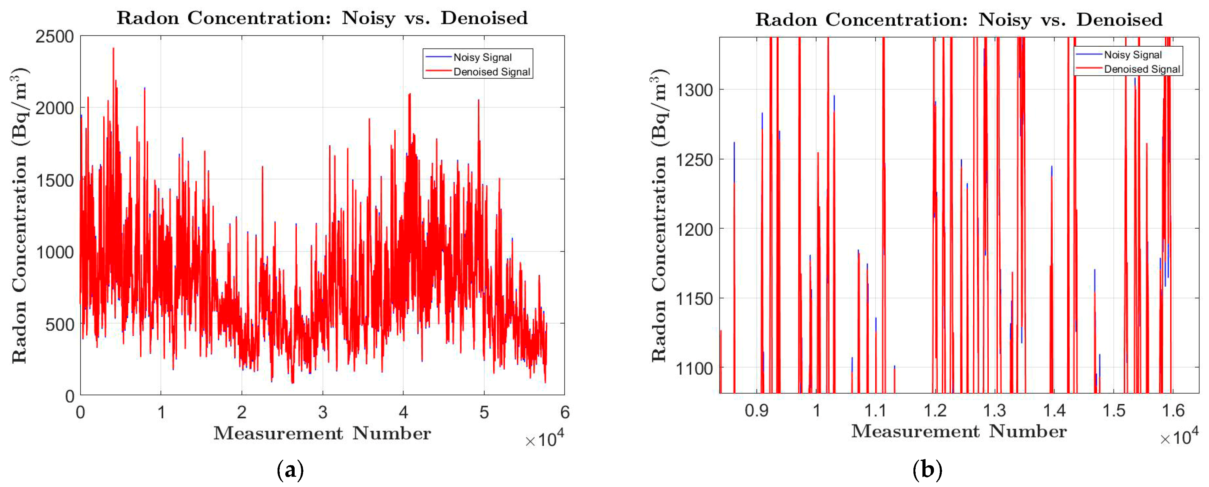
To examine the impact of noise in the sample, the noise was removed using the “Wavelet Signal Denoiser” tool in the MATLAB v2018a environment. The noise removal process with this tool involves transforming the data and includes the following steps:

• The signal is represented in the time–frequency domain through wavelet transformation.
• Noise is identified and analyzed in the time–frequency domain.
• Based on the noise analysis, parts of the signal deemed to contain noise are filtered or removed.
• The wavelet transformation is inverted to return to the original time-domain signal, but with the noise removed.

To achieve optimal noise reduction, several options were used for tuning the filter and wavelet parameters:

• A symmetric wavelet of order 4 (sym4) was used for the signal decomposition function.
• The signal was decomposed 13 times during wavelet decomposition, ultimately resulting in 13 levels.
• The “Bayes” method was applied to distinguish between the noise and the actual signal.
• The median of the difference between the wavelet coefficients and the estimated noise value was used to determine the threshold.
• The noise parameter was set to “Noise: Level Independent,” meaning that the noise was considered independent of the decomposition level.

Figure 4 shows the data for the measured radon concentrations after noise removal.

The choice of sym4 and 13 levels of decomposition was made to maximize noise suppression efficiency while preserving the structural information of radon concentration anomalies. This approach allowed for better representation of actual variations in the data and minimized artifacts that could potentially affect the analysis performed by the neural networks. A symmetric wavelet function (sym4) was selected because it provides an optimal balance between time and frequency localization—wavelet functions from the “symlet” family are modified versions of Daubechies wavelets (Db) but with improved symmetry. In our case, symmetry is crucial, as it reduces phase distortions, which could otherwise impact signal reconstruction accuracy. Additionally, sym4 allows for minimal boundary distortion. Unlike other wavelet functions such as Daubechies (Db) or Coiflet (coif), sym4 ensures a smoother signal reconstruction and reduces edge artifacts in the time series.

Since wavelet transformation is applied to a dataset with a large number of measurements (57,740), we have the capability to use deeper decomposition levels. This is why we chose 13 levels of decomposition. A preliminary analysis of radon time series revealed that the primary fluctuations related to radon concentration are retained in the lower-frequency components (detail coefficients at levels 10–13), while high-frequency noise is predominantly present in the first few levels. By using 13 levels, we ensure that most low-frequency radon variations remain in the signal, while high-frequency disturbances are effectively removed. Tests conducted with different decomposition levels showed that, when using fewer than 10 levels, a significant amount of noise remains, whereas using more than 13 levels does not lead to substantial improvement but unnecessarily increases computational complexity. As a result, we ultimately selected 13 levels for the signal decomposition.

The noise removal procedure was applied to all input factors: atmospheric pressure at the measurement location, relative humidity, and temperature. After this process, the input signals exhibit much clearer characteristics, which significantly facilitate the subsequent training of the ANNs.

To compare the training of ANNs in conditions with noisy data and those where the noise has been removed, an experimental group of ANNs was constructed with the same architecture and characteristics as the ANNs in the control group. Once again, the hyperbolic tangent (3) was used in the neurons of the hidden layers, the training was conducted using the Levenberg–Marquardt algorithm, and all 57,597 measurements were divided into three groups: training samples—75% (40,317); validation samples—15% (8640); independent test samples—15% (8640).

Table 7. Partial results for single-layer ANNs from the experimental group, trained on data with noise removed.

Number of Neurons	$\mathit{M}\mathit{S}\mathit{E}$	$\mathit{R}$
8	19,216.11	0.89
9	19,202.39	0.89
10	18,633.62	0.92
…	…	…
50	12,241.97	0.94
…	…	…
153	7716.20	0.98
…	…	…

presents some of the results from the experimental group of ANNs, which correspond to the control group ANNs shown in Table 6. It is evident that the removal of noise from the training samples leads to a significant reduction in the MSE. In the experimental ANN with 153 neurons, the MSE is now 7716, which is several times smaller than the MSE for this architecture when noise is present in the data.

In experiments with multilayer ANNs, the best result was achieved with an eight-layer ANN, each hidden layer containing 15 neurons, yielding an MSE of 2456.79.

Despite the clear advantage of using input–output samples with noise removed, models remain quite complex in terms of architecture when working with large sample sizes (in this case, 57,597). They are slow in both implementation and construction, and the resulting errors are still not small enough to be acceptable.

5. Model for Predicting Radon Levels Through the Construction of Multiple ANNs

Very often, with large sample sizes, ANNs develop complex architectures where the number of layers and neurons is large. The training error can remain high despite the large number of neurons, due to the strong indeterminacy of the target function in relation to the predictors used. Theoretically, an ANN model that covers all the data from a large sample is convenient because, once created, it can be used for interpolation across the entire sample, as well as for extrapolation beyond its limits. However, from a practical standpoint, this can sometimes be unnecessary.

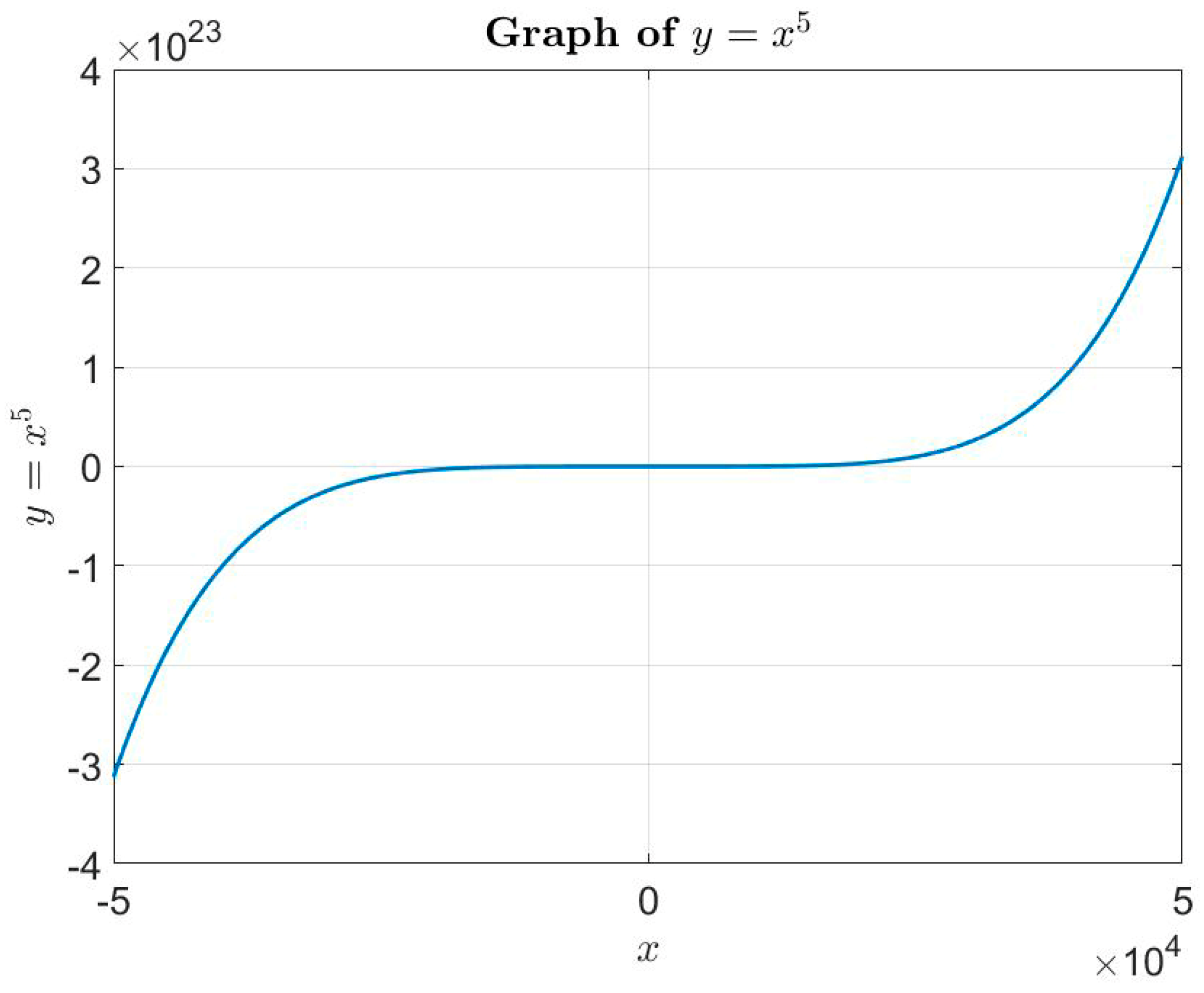
Imagine having a sample of $100$,$000$ instances for approximating a target function, such as $y=x^5$, distributed across the segment $[-\mathrm{50,000}, \mathrm{50,000}]$ (Figure 5). If the practical need is to predict the value of the target function at a point within the sample, for instance at point $x=4.7$, there is no need to train the model to return results at far-off points like $x=\mathrm{47,899}$. If we have a sufficiently rich set of samples in the vicinity of $x=4.7$, we could use them to create an accurate model that describes a much smaller segment, perfectly suited to our needs.

5.1. Algorithms for Building and Using Multiple ANNs for Predicting Soil Radon

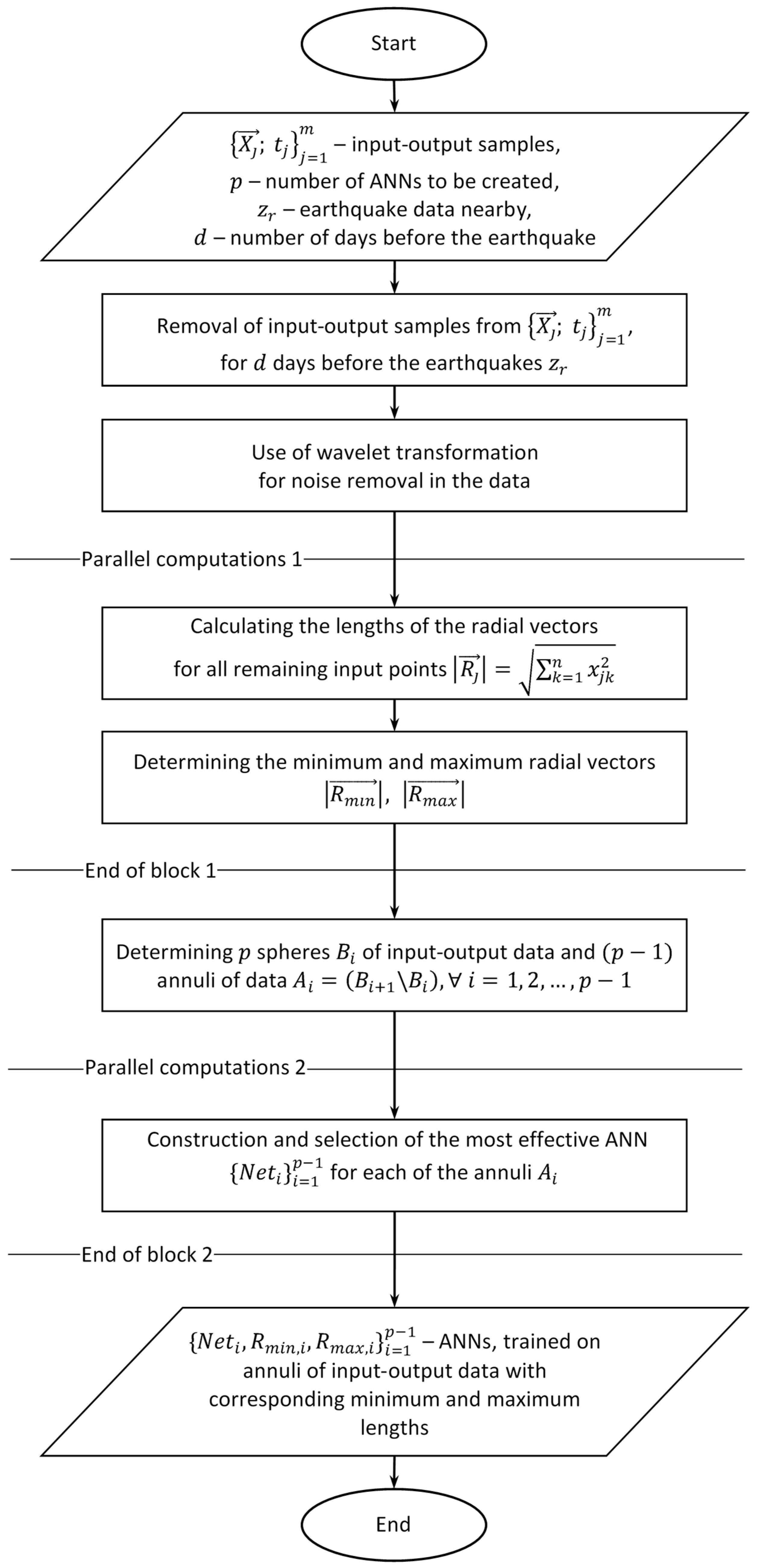
The method we propose consists of creating a set of ANNs, each operating within different ranges of samples characterized by large volume and a high level of indeterminacy. Figure 6 presents a schematic of the algorithm for building multiple ANNs, each trained on separate multidimensional annuli of the input–output data.

Key steps in the algorithm for building multiple ANNs to predict soil radon levels for a given station are:

• Set the required parameters:

  ○

  Input–output data, including date and time of measurements, humidity, temperature, atmospheric pressure, and radon (selected as the target variable);

  ○

  number of predictive ANNs;

  ○

  earthquake data during the period of the input–output data;

  ○

  number of days before the earthquakes for which input–output data will be removed.

• Remove input–output samples for the specified number of days before the earthquakes. This ensures that only input–output data potentially unaffected by processes preceding an upcoming earthquake are used. For more universal use, the number of days is set as a parameter in the algorithm.
• Remove noise from the data, using appropriate wavelet transformations for this purpose.
• Calculate the radial vectors of all input samples.
• Divide the input–output data into annuli, based on the lengths of the radial vectors.
• Build multiple ANNs on each of the annuli and select the most effective one, which will be used for prediction.

As a result of the algorithm, the most effective ANN is selected for each of the annuli, which is then used to predict radon values for new input samples. Some activities within the model—such as independent calculations of vector lengths and ANN training—can be performed either iteratively or in parallel, depending on the available computational resources. Parallel computations would significantly accelerate the training process of the ANNs.

The prediction process is shown in Figure 7. For each new input sample, the length of its radial vector is first calculated. Based on this length, the appropriate ANN from the constructed set of ANNs is selected. The radon level is then predicted using the chosen ANN.

By applying this procedure to all measured points that were not used in building the ANNs, it will be possible to determine whether there are clear dependencies that suggest the potential for real-time earthquake prediction.

5.2. Mathematical Aspects of the Model

The key aspects of the mathematical model of the algorithm are related to:

• Dividing the sample into subsamples;
• Constructing a set of ANNs;
• Predicting the value of the target function.

5.2.1. Dividing the Sample

Let the sample of input–output pairs be given as:

$${\left\{\left[x_{j1},x_{j2},\dots ,x_{jn}; t_j=F\left(x_{j1},x_{j2},\dots ,x_{jn}\right)\right]\right\}}_{j=1}^m.$$

(5)

Each sample consists of an ordered n-tuple of input data $\overrightarrow{X_j}={ (x}_{j1},x_{j2},\dots ,x_{jn})$ and its corresponding functional value of the target function $t_j=F\left(\overrightarrow{X_j}\right)$. If we use a coordinate system with the origin at point $O \left(0, 0,\dots , 0\right)$, then each point ${(x}_{j1},x_{j2},\dots ,x_{jn})$ in the input data, located in the $n$-dimensional predictor space, corresponds to a radial vector $\overrightarrow{R_j}$ with the following length:

$$\left|\overrightarrow{R_j}\right|=\sqrt{{\sum }_{k=1}^n{x}_{jk}^2}, \forall j=\mathrm{1,2},\dots ,m.$$

(6)

Let $\overrightarrow{R_{max}}$ and $\overrightarrow{R_{min}}$ denote the radial vectors with the largest and smallest lengths, respectively, i.e.,

$$\left|\overrightarrow{R_{max}}\right|={\max \left(\left|\overrightarrow{R_j}\right|\right)}_{j=1}^m,$$

(7)

$$\left|\overrightarrow{R_{min}}\right|={\mathit{min}\left(\left|\overrightarrow{R_j}\right|\right)}_{j=1}^m,\forall j=1, 2,\dots , m.$$

(8)

The sphere $B_p\left(O, \left|\overrightarrow{R_{max}}\right|\right)$ is divided into $(p-1)$ $n$-dimensional annuli through nested spheres with the center at the origin of the coordinate system:

$$B_1\subset B_2\subset B_3\subset \dots \subset B_p,$$

(9)

where $B_1\left(O,\left|\overrightarrow{R_1}\right|\right)$, and for any two spheres $B_i\left(O,\left|\overrightarrow{R_i}\right|\right)$ and $B_{i+1}\left(O,\left|\overrightarrow{R_{i+1}}\right|\right)$, satisfies the condition $\left|\overrightarrow{R_i}\right|<\left|\overrightarrow{R_{i+1}}\right|,\forall i=1,2,\dots ,p-1$. Each of the annuli $A_i=(B_{i+1}\backslash B_i)$ contains the points from the predictor sample with radial vectors whose lengths lie in the interval $\left[\left|\overrightarrow{R_i}\right|,\left|\overrightarrow{R_{i+1}}\right|\right]$.

5.2.2. Constructing a Set of ANNs

At this stage of the algorithm, a set of $p-1$ different ANNs ${\left\{{Net}_i\right\}}_{i=1}^{p-1}$ is constructed, where each ANN ${Net}_i$ is trained on data from the annulus $A_i$, i.e., on samples from the dataset (5), for which:

$$\left|\overrightarrow{R_i}\right| \le \sqrt{{\sum }_{k=1}^n{x}_{rk}^2} \le \left|\overrightarrow{R_{i+1}}\right|, \forall i=1, 2,\dots ,p-1 и 1 \le r \le m.$$

(10)

The overall $MSE$ of the set of ANNs is

$$MSE={\displaystyle \frac{\sum _{i_1=1}^{q_1}{({C_{Rn}}_{i_1}-\widehat{{C_{Rn}}_{i_1}})}^2+\sum _{i_2=1}^{q_2}{({C_{Rn}}_{i_2}-\widehat{{C_{Rn}}_{i_2}})}^2+\dots \sum _{i_{p-1}=1}^{q_{p-1}}{({C_{Rn}}_{i_{p-1}}-\widehat{{C_{Rn}}_{i_{p-1}}})}^2}{q_1+q_2+\dots +q_{p-1}}},$$

(11)

where $q_i$ is the number of samples in each annulus $A_i$, and ${C_{Rn}}_{i_j}$ and $\widehat{{C_{Rn}}_{i_j}}$ are the actual and predicted radon concentrations by the ANNs for each sample in the annulus, respectively.

Given that the sum of the samples in all annuli is actually equal to the total sample size, i.e.,

$$\sum _{i=1}^{p-1}{q}_i=m$$

(12)

it follows that

$$MSE={\displaystyle \frac{1}{m}}\sum _{j=1}^{p-1}\sum _{i=1}^{q_j}{({C_{Rn}}_{i_j}-\widehat{{C_{Rn}}_{i_j}})}^2.$$

(13)

5.2.3. Predicting the Value of the Target Function

When it is necessary to predict the value of the target function at a new point ${(x}_1,x_2,\dots x_n)$ the algorithm calculates the length of the radial vector of the point in the predictor space:

$$\left|\overrightarrow{R_i}\right|=\sqrt{{\sum }_{k=1}^n{x}_k^2}.$$

(14)

Then, the algorithm selects the ANN ${Net}_q\in {\left\{{Net}_i\right\}}_{i=1}^{p-1}$, which was trained in the region of the $n$-dimensional annulus $A_q$ that contains the point ${(x}_1,x_2,\dots ,x_n)$, and performs the prediction using that ANN.

6. Experiments

The main expectations during the experiments are:

• Predictions of radon quantities for the input–output samples that were removed from the training data due to approaching earthquakes will differ from the actual measured values of the target variable.
• Depending on the stations, the influence of the predictors on radon levels will vary in strength.

  ○

  It is possible that at some stations there will be a clear difference between the measured and predicted radon values, while at others, the difference may be minimal.

  ○

  It is possible that at some stations the predicted radon levels will be higher than the measured ones, at others they may be lower, and at some, there may be no significant difference.

In the conducted experiments, we divide the space containing all the points from the real sample into several annuli, each with an equal number of input–output data points. The data in the sample are for:

• atmospheric pressure at the measurement location $Ap \left(\mathrm{h}\mathrm{P}\mathrm{a}\right)$;
• relative humidity $Rh (\%)$;
• temperature $T (°\mathrm{C})$.

When dividing into 10 annuli, each group of input–output samples consists of 5760 elements, and when divided into 20 annuli, each group consists of 2880 elements. The input–output samples from each annulus are further divided into groups used for the creation of the corresponding ANN: training—75%; validation—15%; independent test—15%.

Table 8. Partial results from training single-layer ANNs on one of the annuli, when dividing the predictor space into 10 and 20 annuli.

Number of Neurons	Results for 1 of the 10 Annuli		Results for 1 of the 20 Annuli
	$\mathit{M}\mathit{S}\mathit{E}$	$\mathit{R}$	$\mathit{M}\mathit{S}\mathit{E}$	$\mathit{R}$
8	6052.68	0.87	3661.32	0.90
9	5451.17	0.89	3341.62	0.93
10	5148.43	0.91	3048.93	0.94
…	…	…	…	…
50	1982.38	0.97	882.66	0.98
…	…	…	…	…
153	892.61	0.98	641.25	0.99
…	…	…	…	…

describes the results from training single-layer ANNs in two specific regions $(B_2\backslash B_1)$, when dividing the space into 10 and 20 annuli. The results for other regions are similar, indicating that ANNs become more efficient with a larger number of annuli (and consequently a smaller number of input–output samples per annulus) and with an increase in the number of neurons. Of course, both the number of neurons and the number of input–output samples have critical limits, which have been explored in various literature sources [51,52].

The experiments conducted with multilayer ANNs also showed a significant reduction in error. For example, with 10 annuli, the $MSE$ for a six-layer ANN with 53 neurons in each layer is only 2.68 units. Similarly, with 20 annuli, the $MSE$ for the same six-layer ANN with 53 neurons per layer decreases to 1.7 units.

To evaluate the effectiveness of this approach, a comparative analysis was conducted using four popular regression models:

i.

Linear Regression (LR). One of the most basic methods, which assumes a linear relationship between the input parameters (atmospheric pressure, temperature, and humidity) and radon concentration. Given the strong linear correlation between radon concentration and atmospheric pressure, as well as the moderate correlation with temperature, we were particularly interested in examining the results of LR and ARIMA.

ii.

ARIMA. An auto regressive integrated moving average model, widely used for time series analysis and forecasting. The selected model, ARIMA(1,1,1), includes one autoregressive term, one differencing step, and one moving average term.

iii.

Random Forest (RF). An ensemble model based on multiple regression trees (a 100-tree ensemble was used in this case), where the mean prediction is taken to improve the model’s stability.

iv.

Support Vector Regression (SVR). A regression model that applies non-linear transformations using radial basis function (RBF) kernels to determine the optimal hyperplane for predicting radon values.

v.

Artificial Neural Network. The ANN model consists of six layers with 53 neurons per layer and is trained using the backpropagation algorithm.

The comparison of the models is based on the mean squared error (MSE), and the comparative analysis itself was conducted under two main scenarios:

1.

Prediction across the entire region

The ANN and the other models were trained and tested on the entire dataset, using atmospheric pressure, temperature, and humidity as input parameters.

2.

Prediction after spatial segmentation of input parameters

The input parameter space was divided into 20 separate ring-shaped zones (annuli). The ANN and the alternative models were trained and validated separately for each zone to assess how segmenting the input factors affects prediction accuracy.

Table 9. Model errors during training and prediction across the entire region (${MSE}_{Global}$) and after segmenting the feature space into 20 annuli (${MSE}_{Segmented}$).

Model	$\mathbf{L}\mathbf{i}\mathbf{n}\mathbf{e}\mathbf{a}\mathbf{r} \mathbf{R}\mathbf{e}\mathbf{g}\mathbf{r}\mathbf{e}\mathbf{s}\mathbf{s}\mathbf{i}\mathbf{o}\mathbf{n}$	$\mathbf{A}\mathbf{R}\mathbf{I}\mathbf{M}\mathbf{A}$	$\mathbf{R}\mathbf{a}\mathbf{n}\mathbf{d}\mathbf{o}\mathbf{m} \mathbf{F}\mathbf{o}\mathbf{r}\mathbf{e}\mathbf{s}\mathbf{t}$	$\mathbf{S}\mathbf{V}\mathbf{R}$	$\mathbf{A}\mathbf{N}\mathbf{N}$
${MSE}_{Global}$	$4801$	$1.682\times {10}^3$	$2749$	$3152$	$2856.79$
${MSE}_{Segmented}$	12.411	3429	8.47	10.59	1.7

presents the results of the comparative analysis.

When the models are applied directly to the entire dataset (${MSE}_{Global}$), the best performance is observed in random forest and ANNs. The ARIMA model produces the weakest results, indicating that the previously observed linear dependencies in the data are insufficient for accurate predictions. This somewhat justifies our decision to retain air humidity as a variable in the model. After spatial segmentation (${MSE}_{Segmented}$), the ANN once again achieves the lowest error (1.7), significantly improving its results compared to other models. Linear regression and support vector regression also show improvements, but do not reach the accuracy of the ANN. Random forest achieves a relatively good MSE (8.47) but still lags behind the ANN in terms of accuracy.

Thus, the final conclusion is that the ANN outperforms all the alternative models considered, especially after the spatial segmentation of the factors. The segmentation of the feature space into annular zones improves the predictive accuracy of all models, but the effect is most pronounced in the ANN (MSE reduction from 2856.58 to 1.7). ARIMA shows the weakest results, suggesting that radon concentrations do not simply follow linear time-dependent processes but instead depend on complex non-linear interactions, which the ANN successfully captures.

Before presenting the test results, it is important to note that both the training and testing of the ANN models were performed on data that had been pre-denoised using wavelet transformation. The predicted radon concentration is compared with actual measurements, which have also undergone wavelet filtering, without the need for reconstruction or the addition of filtered noise components. This ensures full compatibility between the ANN output and the data used for evaluation.

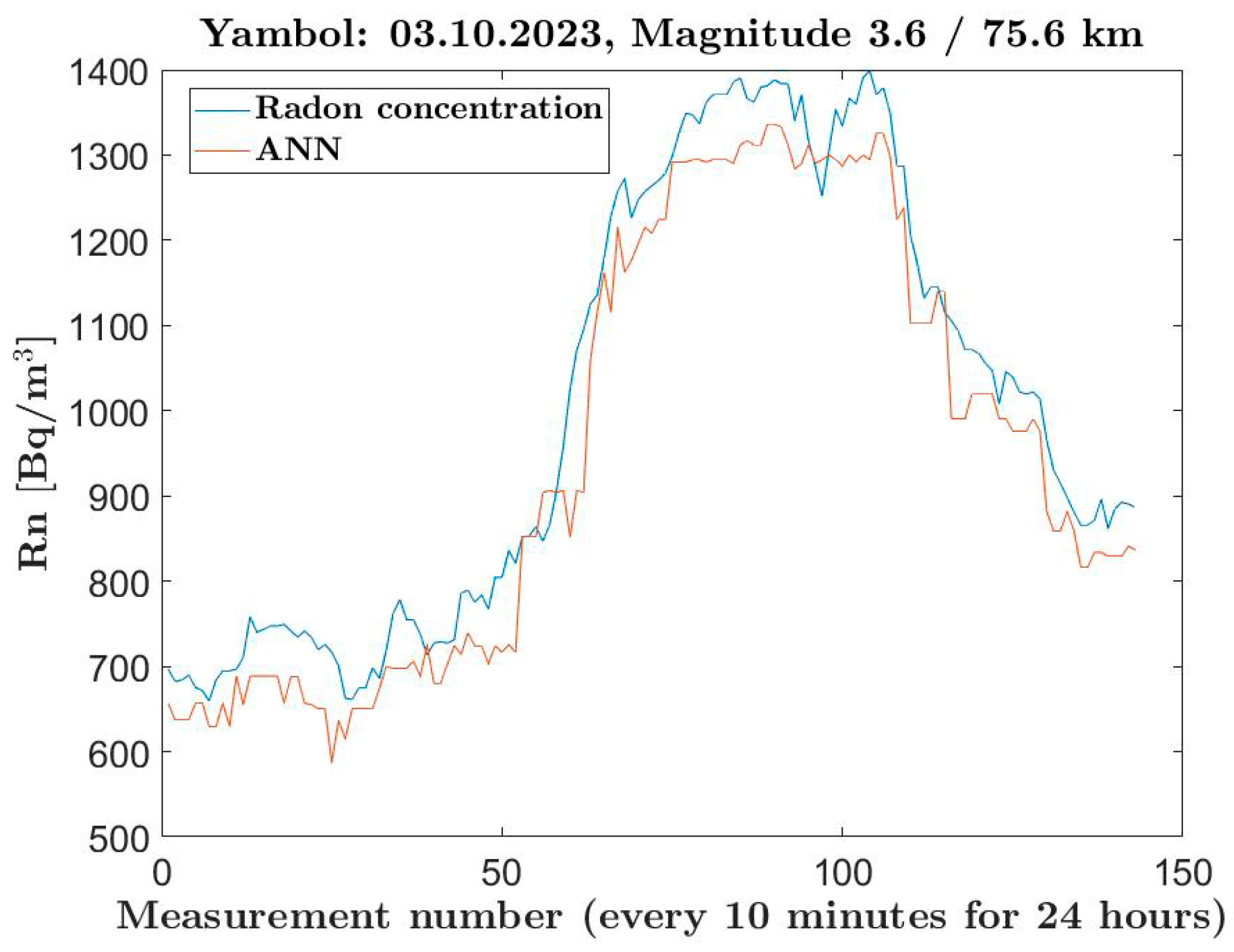
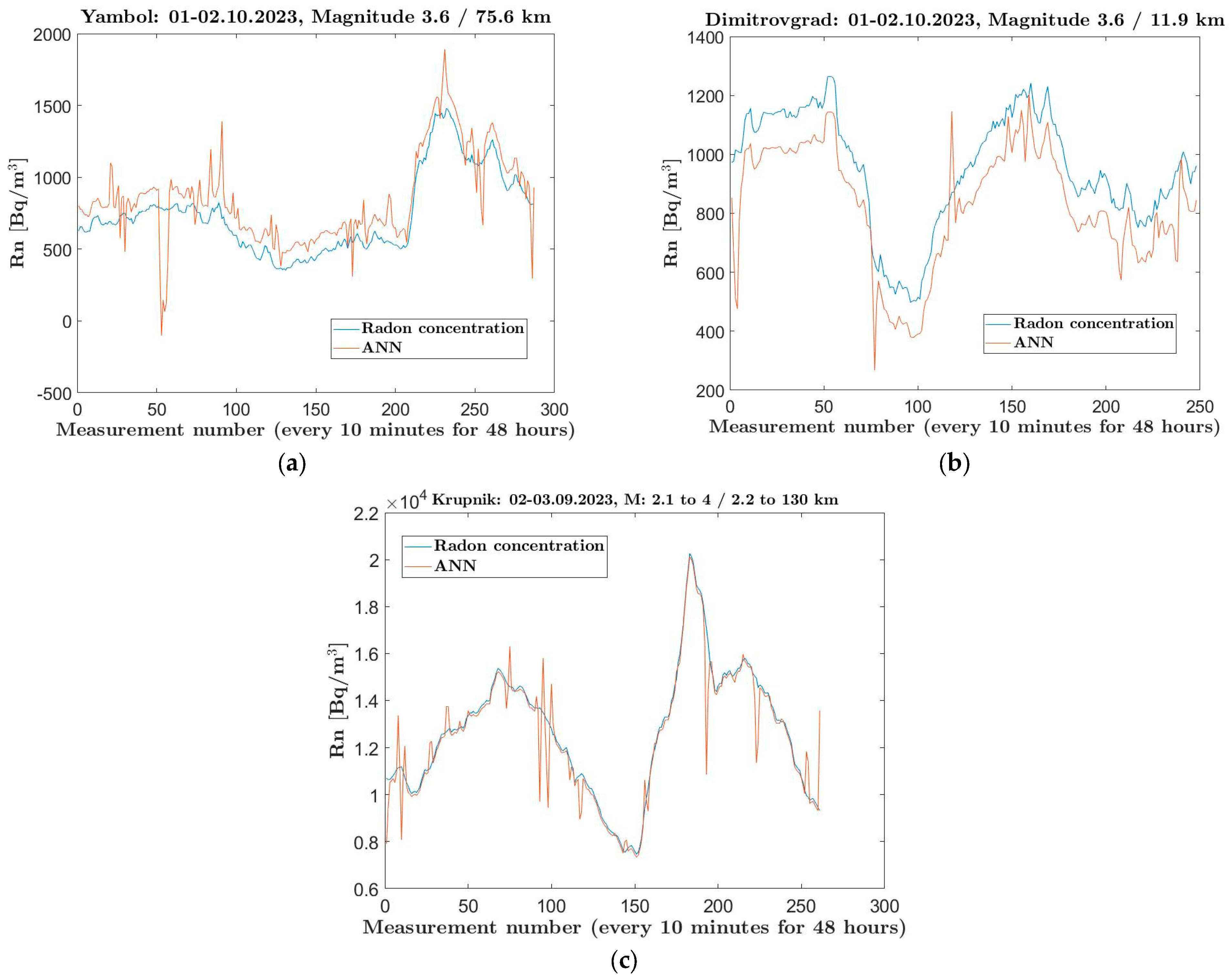
To test the method, we selected data measured at the Yambol station on 3 October 2023, when an earthquake with a magnitude of 3.6 was recorded 75.6 km away. We chose to use a set of 10 single-layer ANNs with 153 neurons, trained with the Levenberg–Marquardt algorithm in the 10 annuli of the initial sample of 57,957 instances. After submitting the test sample of 143 measurements from the day of the earthquake, the radial vectors of the input points were determined, which fell into seven of the annuli, and predictions were made using the seven ANNs trained in these regions. According to the models, fluctuations (Figure 8) in radon concentration (the red line) were observed between 671.34 Bq/m³ and 1260.01 Bq/m³, with an average value of 950.72 Bq/m³. The actual radon measurements at the Yambol station for these values were 695.34 Bq/m³ and 1398.97 Bq/m³, with an average value of 1002.70 Bq/m³. An important conclusion from this is that, on the day of the earthquake, the measured radon concentrations were higher than the predicted normal levels by the model.

Similar studies for the earthquake on October 3 2023 have been conducted for the Dimitrovgrad station ($Latitude\_GPS=42.054814$, $Longitude\_GPS=25.6051$), which is located 11.9 km from the earthquake’s epicenter. A total of 112 measurements were taken at this station.

When applying the set of ANNs, slightly elevated real radon levels are again observed (Figure 9a) compared to the predicted normal levels by the ANNs.

In contrast to the two mentioned stations, at the Krupnik station ($Latitude\_GPS=41.84748$; $Longitude\_GPS=23.11773$), lower radon levels were observed on the day of a nearby earthquake. On 4 September 2023, multiple earthquakes (17 in total) with magnitudes ranging from 2.1 to 4 were detected, with epicenters located between 2.2 and 130 km from the Krupnik station. Eleven of these quakes had epicenters less than 10 km away. Under these circumstances, contrary to expectations, the actual radon levels were lower than those predicted as normal by the ANNs (Figure 9b). The actual measured radon concentration ranged between 7743 and 20,433 Bq/m³, with an average value of 15,322.92 Bq/m³, while the ANNs’ prediction for normal behavior of radon concentration indicated higher values: approximately 4249 to 27,107 Bq/m³, with an average of 16,688.80 Bq/m³.

These differences in radon anomalies at Krupnik compared to the other stations can be explained by the influence of multiple factors. Krupnik is located in southwestern Bulgaria, near the Kresna Gorge, which is part of the active seismic zone Krupnik-Kresna. This area is known for its complex fault system and high seismic activity. According to Dobrev, the Krupnik-Kresna zone has been the subject of long-term 3D monitoring of active fault structures, highlighting its tectonic complexity and significance [53].

In contrast, Yambol and Dimitrovgrad are located in southeastern Bulgaria, within the Upper Thracian Lowland. This area is also intersected by fault structures, but they are not as active or complex as those in Krupnik. According to the River Basin Management Plan for the East Aegean Region [54], superimposed grabens have formed in the Upper Thracian Depression, filled with neogene and quaternary materials, shaped by major tectonic faults. These geological differences may explain the observed variations in radon concentration behavior between the stations. The complex fault system in the Krupnik area may influence subsurface gas flows, leading to different radon emission behavior compared to the more stable tectonic conditions in Yambol and Dimitrovgrad.

Furthermore, the Krupnik area has documented groundwater presence, confirmed in the Register of Hydrogeological Points from the Quantitative Groundwater Monitoring Network, maintained by the National Institute of Meteorology and Hydrology. This register even lists a tube well in Krupnik with coordinates 41°51′8.355″ N latitude and 23°7′5.856″ E longitude, located within the Struma River Basin [55]. These hydrological conditions may also influence the behavior of radon gas—it is well known that groundwater can retain or dilute radon before it is released into the atmosphere. This could explain why the measured radon concentrations in Krupnik are lower than expected, compared to the predictions of the ANN model.

In addition to geological and hydrological factors, it is important to note that 17 earthquakes of varying magnitudes occurred in Krupnik during the observed periods, making the process even more complex. It is possible that some of these earthquakes caused different shifts in the Earth’s layers and changes in gas flows, leading to a dispersion of radon in different directions rather than a clear, unambiguous increase in concentration.

The results from applying the same approach for the 48 h period prior to the day of the considered earthquakes are presented in Figure 10.

The results show elevated levels of actual radon concentrations during the 48 h period before the earthquake at the Dimitrovgrad and Krupnik stations. At the Yambol station, however, the actual radon concentrations recorded 48 h before the earthquake were lower than those predicted as normal by the set of ANNs.

The obtained results show that, despite some deviations, the ANNs are able to capture the trend in radon behavior. This indicates that the artificial neurons have identified a pattern in the progression of radon concentration from the preceding and following days and are able to interpolate it for time periods they were not trained on. However, the captured trend may suggest that, in addition to the presumed dependence of radon concentration on earthquakes, there is another factor that strongly influences radon levels, even during periods without seismic activity.

7. Conclusions

The proposed model for dividing input–output data into multidimensional annuli for building multiple ANNs accelerates the training process and creates more efficient ANNs. While training a single ANN on all the input–output data is a time-consuming process that requires extensive resources, training multiple ANNs on smaller datasets allows for the development of a faster and more efficient algorithm. The model enables the use of parallel computations during both the construction and utilization of individual ANNs, further enhancing the overall performance and speed. Another positive aspect of the proposed model is that all ANNs, except for the first and last, are used for interpolation in the prediction process, which helps reduce errors. Extrapolation is only expected with the first and last networks when making predictions for points outside the range of the input samples. In practice, one of the greatest advantages of the proposed model is in single-point predictions or predictions for sets of points with similar radial vectors. In such cases, only one ANN trained in the corresponding annulus can be used, eliminating the need for modeling an ANN trained on the entire initial dataset, which could be of considerable size.

The proposed method is not suitable for small samples or for creating multiple annuli with small samples, as this would result in inefficient ANNs. An interesting problem in this context is finding a function that determines the optimal number of annuli into which a given sample of input–output data should be divided. This would help balance the size of the sample with the performance of the ANNs, ensuring that the model remains both efficient and accurate. The conducted studies make it difficult to provide a definitive answer to the question of whether elevated radon levels are a reliable indicator of an impending earthquake. While the one-day forecasts for the Yambol and Dimitrovgrad stations confirm the preliminary expectation that rising radon levels may be considered an indicator of an earthquake, the opposite behavior is observed at the Krupnik station—decreasing radon levels—even in the presence of multiple nearby tremors. The two-day forecasts for the earthquakes and stations under consideration also do not provide a clear answer regarding radon concentration behavior.

Future research involving multiple earthquakes and a larger number of stations will reveal whether the observed results are consistent for each individual station, i.e., whether there is or is not a relationship between radon levels and an approaching earthquake at different stations. Although external atmospheric influences have been minimized at the stations studied, it would be appropriate to also investigate the impact of seasonal changes as a factor influencing radon concentration. Another future objective set by the team is related to Bayesian methods, which could be useful for further quantifying the probability of radon anomalies before earthquakes. Our idea is to develop models that reassess probabilities based on new measurements, thus providing a more dynamic approach to analyzing radon concentration time series. Furthermore, we consider it highly beneficial to combine ANNs with Bayesian methods, where the latter would serve as a posterior assessment of the reliability of ANN predictions, adding probabilistic bounds to the forecasted anomalies. We believe that such an approach would enhance the robustness and reliability of predictive models, particularly in the context of varied geological and climatic conditions.