Characterization of Finsler Space with Rander’s-Type Exponential-Form Metric

Abstract

This study explores a unique Finsler space with a Rander’s-type exponential metric, $\mathcal{G}(\alpha ,\beta )=(\alpha +\beta )e^{{\displaystyle \frac{\beta }{(\alpha +\beta )}}}$, where $\alpha$ is a Riemannian metric and $\beta$ is a 1-form. We analyze the conditions under which its hypersurfaces behave like hyperplanes of the first, second, and third kinds. Additionally, we examine the reducibility of the Cartan tensor $\mathcal{C}$ for these hypersurfaces, providing insights into their geometric structure.

1. Introduction

The study of Finslerian hypersurfaces and their classification represents a significant advancement in the field of Finsler geometry, a branch of differential geometry that generalizes Riemannian geometry by allowing the metric to depend not only on position but also on direction. The notion of Finslerian hypersurfaces was first introduced by the eminent mathematician Matsumoto, who provided a systematic classification of these hypersurfaces into three distinct types: hyperplanes of the first kind, second kind, and third kind. This classification was based on the geometric and algebraic properties of the hypersurfaces and their relationship to the underlying Finsler metric. Matsumoto’s work laid the groundwork for subsequent research, inspiring numerous mathematicians to explore the properties of these hypersurfaces under various modifications and generalizations of the Finsler metric. These investigations, as documented in references [1,2,3,4,5,6,7,8,9,10,11,12], have uncovered a rich array of geometric properties, deepening our understanding of the intrinsic structure of Finslerian hypersurfaces and their applications in geometry and physics.

In addition to his contributions to the theory of Finslerian hypersurfaces, Matsumoto also introduced the concept of an $(\alpha ,\beta )$-metric [13], which has since become a central topic of research in Finsler geometry. An $(\alpha ,\beta )$-metric is a generalization of the classical Riemannian metric, where $\alpha$ represents the Riemannian part of the metric and $\beta$ is a 1-form that introduces a directional dependence. The exponential metric, expressed as $L=\alpha e^{{\displaystyle \frac{\beta }{\alpha }}}$, is a unique form of the $(\alpha ,\beta )$-metric that has attracted significant attention due to its elegant structure and its connections to theoretical physics and cosmology. The exponential metric has been extensively examined by various authors [14,15,16,17,18,19,20], who have explored its geometric properties under different conditions. One notable feature of the exponential metric is its relationship to Rander’s metric. Specifically, under certain transformations, the exponential metric can be reduced to Rander’s metric, which has significant applications in theoretical physics, particularly in the study of spacetime geometries and cosmological models. This connection highlights the importance of $(\alpha ,\beta )$-metrics not only in pure mathematics but also in applied fields.

A hypersurface is a generalization of the concept of hyperplane. It is defined as follows.

Definition 1. 

A sub-manifold of dimension $(n-1)$ is termed a hypersurface of an enveloping manifold $\mathcal{M}$ of dimension n, and the co-dimension of the hypersurface is one.

If $m>n$, then the space $V^n$ is termed a subspace of $V^m$, and $V^m$ serves as an enveloping space for $V^n$. Particularly, if $m=n+1$, then $V^n$ is referred to as a hypersurface of the enveloping space $V^{n+1}$.

Hence, a hypersurface ${\mathcal{M}}^{n-1}$ of the manifold ${\mathcal{M}}^n$ can be parametrically described by the equation

$${\mathtt{x}}^i={\mathtt{x}}^i\left({\mathtt{u}}^{\alpha }\right),\{\alpha =1,2,\dots ,(n-1\left)\right\},$$

where u represent the Gaussian coordinates on the hypersurface $M^{n-1}$.

If ${\mathbf{y}}^i$ represents the supporting line element at a point $\left({\mathbf{u}}^{\alpha }\right)$ on the hypersurface ${\mathcal{M}}^{n-1}$, tangential to ${\mathcal{M}}^{n-1}$, then we have

$${\mathtt{y}}^i={\mathcal{B}}_{\alpha }^i\left(u\right)v^{\alpha }$$

Thus, ${\mathbf{v}}^{\alpha }$ is regarded as the supporting element of $M^{n-1}$ at a point $\left({\mathbf{u}}^{\alpha }\right)$. Considering the function $\underline{\mathcal{G}}(u,v)=\mathcal{G}(x\left(u\right),y(u,v))$, which generates a Finsler metric on ${\mathcal{M}}^{n-1}$, we obtain an $(n-1)$-dimensional Finsler space ${\mathcal{U}}^{(n-1)}=({\mathcal{M}}^{n-1},\underline{\mathcal{G}}(u,v))$.

In Finsler geometry, a hyperplane can be classified into different types based on its geometric properties. Below are some examples of such hypersurfaces:

Example 1. 

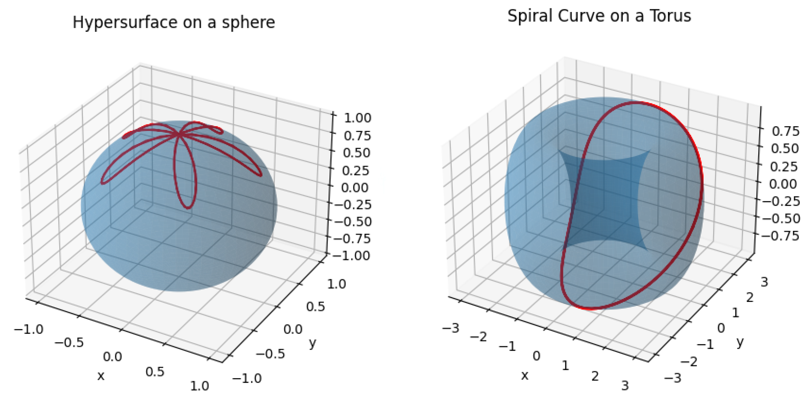
A sphere can be visualized as a three-dimensional structure and is an example of a two-dimensional manifold $(n=2)$ embedded in three-dimensional space. Thus, a hypersurface on this sphere would be a one-dimensional curve.

Example 2. 

A torus can be visualized as a three-dimensional structure and is an example of a two-dimensional manifold $(n=2)$ embedded in three-dimensional space, and a spiral curve would represent the hypersurface.

In Figure 1, the first image shows the sphere as the three-dimensional space, with the curve (red lines) representing a hypersurface within it. The second image features a torus as the three-dimensional space, where the spiral curve (red line) represents a hypersurface within that structure.

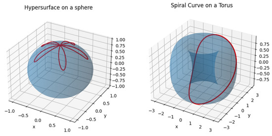
Figure 1. Examples of hypersurface in sphere and torus.

Example 3 

(Hyperplane of first kind). A hyperplane in a three-dimensional Finsler space is classified as a “hyperplane of the first kind" if it intersects with a given curve or surface within that space.

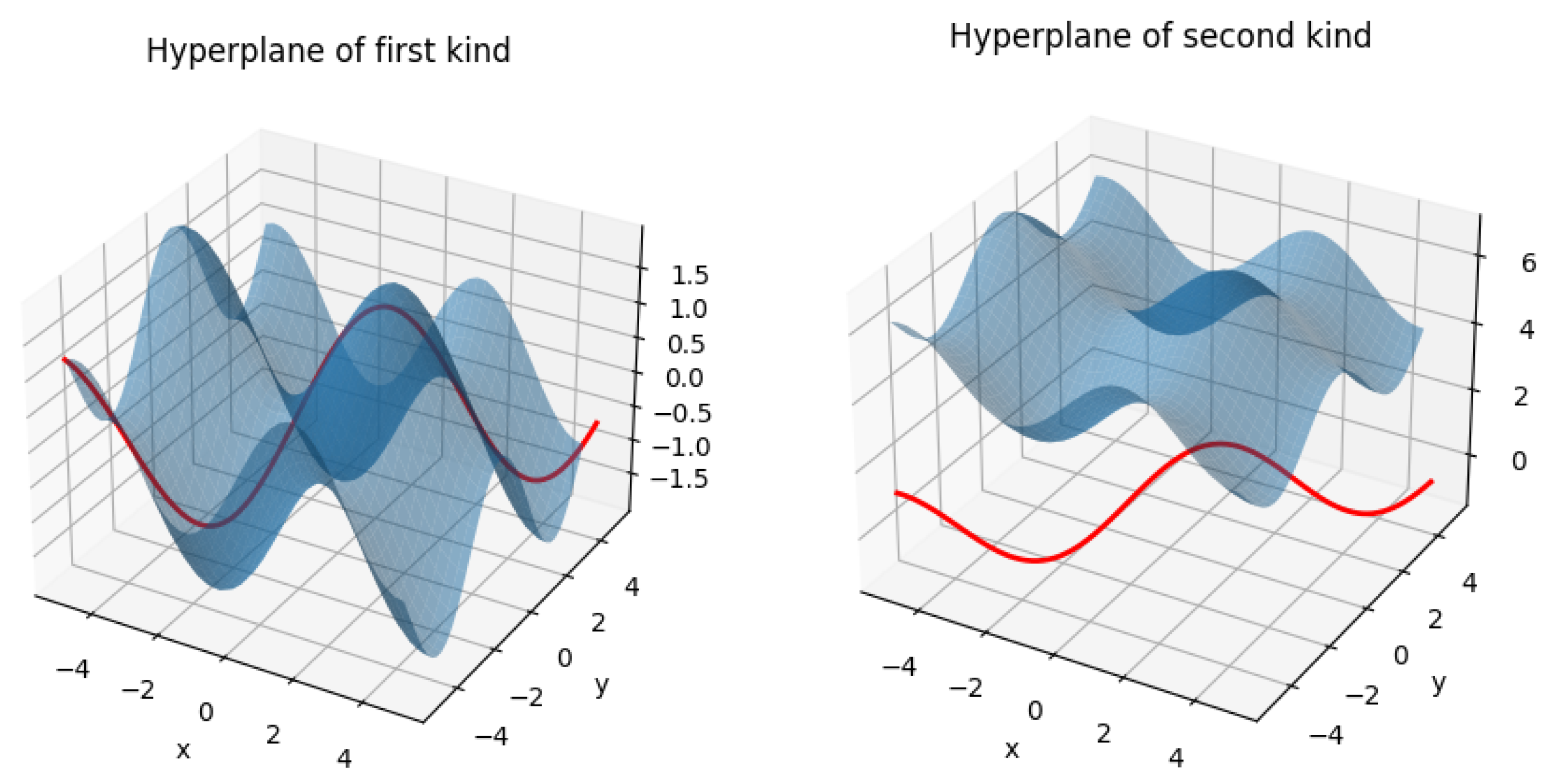
Example 4 

(Hyperplane of second kind). A “hyperplane of the second kind" in Finsler geometry is a hyperplane (represented by a surface) that does not intersect with a given curve or surface in the three-dimensional Finsler space.

In Figure 2, the first image shows a hyperplane intersecting with a curve, and this intersection is classified as a “hyperplane of the first kind”. In the second image, the surface is shifted upward by adding 5 to the z-values, preventing any intersection with the curve. This is referred to as the “hyperplane of the second kind”.

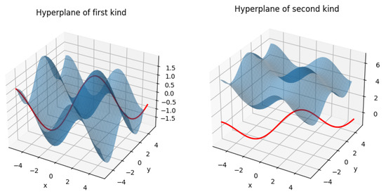
Figure 2. Examples of first- and second-kind hyperplane in 3D.

Example 5 

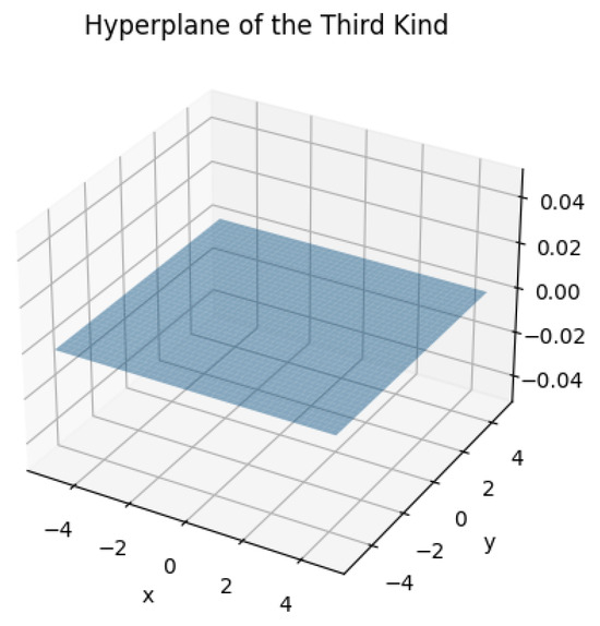
(Hyperplane of third kind). We consider a flat plane embedded in 3D space. This plane has zero curvature, and its normal vector remains constant. This serves as a simplified analogy for a hyperplane of the third kind in Finsler geometry, where the conditions of vanishing curvature and tensor create a similar “flatness" within the Finsler space (Figure 3).

Figure 3. Example of hyperplane of third kind.

Thus “hyperplane of the third kind” is essentially “flat” with respect to the ambient Finsler space.

In this paper, we introduce and analyze a novel $(\alpha ,\beta )$-metric defined as $\mathcal{G}(\alpha ,\beta )=(\alpha +\beta )e^{{\displaystyle \frac{\beta }{(\alpha +\beta )}}}$. We refer to this metric as the Rander’s-type exponential $(\alpha ,\beta )$-metric due to its structural similarity to Rander’s metric combined with an exponential factor. This metric represents a natural extension of the classical Rander’s metric and the exponential metric, combining their features in a way that opens up new avenues for geometric exploration. Our primary focus is on investigating the intrinsic properties of this Finsler space, particularly the conditions under which its hypersurfaces exhibit characteristics of hyperplanes of the first, second, and third kind. In Theorem 3, we derive the necessary and sufficient conditions for the hypersurfaces of the Rander’s-type exponential $(\alpha ,\beta )$-metric to be classified as hyperplanes of the first kind. These conditions are expressed in terms of the geometric invariants of the Finsler space and provide a clear characterization of the hypersurfaces in this category. Similarly, in Theorem 4, we establish the conditions under which the hypersurfaces exhibit properties of hyperplanes of the second kind. These conditions involve a deeper analysis of the interplay between the Riemannian part $\alpha$ and the 1-form $\beta$ in the metric. Finally, in Theorem 5, we address the case of hyperplanes of the third kind, identifying the specific geometric constraints that must be satisfied for the hypersurfaces to fall into this classification.

In addition to the classification of hypersurfaces, we also investigate the reducibility of the Cartan tensor $\mathcal{C}$ for these hypersurfaces. The Cartan tensor is a fundamental object in Finsler geometry, encoding information about the anisotropy of the Finsler metric. Its reducibility, or the extent to which it can be decomposed into simpler components, provides valuable insights into the geometric structure of the Finsler space. In Propositions 1–3, we examine the reducibility of the Cartan tensor in various forms, focusing on the hypersurfaces associated with the Rander’s-type exponential $(\alpha ,\beta )$-metric. These propositions reveal the conditions under which the Cartan tensor can be reduced to simpler forms, shedding light on the geometric behavior of the hypersurfaces and their relationship to the underlying metric.

Through this detailed analysis, we aim to contribute to the broader understanding of Finslerian hypersurfaces and their geometric properties, particularly in the context of the newly introduced Rander’s-type exponential $(\alpha ,\beta )$-metric. Our results not only extend the existing theory of Finslerian hypersurfaces but also provide new tools for exploring the geometric and physical implications of $(\alpha ,\beta )$-metrics. By uncovering the intrinsic properties of this metric and its hypersurfaces, we hope to inspire further research into the rich and diverse world of Finsler geometry.

2. Preliminaries

In this study, we investigate an n-dimensional Finsler space represented as ${\mathcal{U}}^n=\{{\mathcal{M}}^n,\mathcal{G}(\alpha ,\beta )\}$. Here, ${\mathcal{U}}^n$ consists of an n-dimensional differentiable manifold ${\mathcal{M}}^n$ coupled with a fundamental function $\mathcal{G}$ that takes on a Rander’s-type exponential form within a unique Finsler space metric, expressed as

$$\mathcal{G}(\alpha ,\beta )=(\alpha +\beta )e^{{\displaystyle \frac{\beta }{(\alpha +\beta )}}}$$

(1)

Taking partial derivatives of Equation (1) with respect to $\alpha$ and $\beta$ yields

$${\mathcal{G}}_{\alpha }={\displaystyle \frac{\alpha }{(\alpha +\beta )}}{e}^{{\displaystyle \frac{\beta }{(\alpha +\beta )}}},{\mathcal{G}}_{\beta }={\displaystyle \frac{(2\alpha +\beta )}{(\alpha +\beta )}}{e}^{{\displaystyle \frac{\beta }{(\alpha +\beta )}}}$$

$${\mathcal{G}}_{\alpha \alpha }={\displaystyle \frac{{\beta }^2}{{(\alpha +\beta )}^3}}{e}^{{\displaystyle \frac{\beta }{(\alpha +\beta )}}}{\mathcal{G}}_{\beta \beta }={\displaystyle \frac{{\alpha }^2}{{(\alpha +\beta )}^3}}{e}^{{\displaystyle \frac{\beta }{(\alpha +\beta )}}}$$

$${\mathcal{G}}_{\alpha \beta }=-{\displaystyle \frac{\alpha \beta }{{(\alpha +\beta )}^3}}{e}^{{\displaystyle \frac{\beta }{(\alpha +\beta )}}}$$

where ${\mathcal{G}}_{\alpha }={\displaystyle \frac{\partial \mathcal{G}}{\partial \alpha }},{\mathcal{G}}_{\beta }={\displaystyle \frac{\partial \mathcal{G}}{\partial \beta }},{\mathcal{G}}_{\alpha \alpha }={\displaystyle \frac{\partial \mathcal{G}\alpha }{\partial \alpha }},{\mathcal{G}}_{\beta \beta }={\displaystyle \frac{\partial {\mathcal{G}}_{\beta }}{\partial \beta }},{\mathcal{G}}_{\alpha \beta }={\displaystyle \frac{\partial {\mathcal{G}}_{\alpha }}{\partial \beta }}$.

In the Finsler space ${\mathcal{U}}^n=\{{\mathcal{M}}^n,\mathcal{G}(\alpha ,\beta )\}$, the normalized support element $l_i=\dot{{\partial }_i\mathcal{G}}$ and the angular metric tensor ${\mathtt{h}}_{ij}$ are defined as, per reference [21],

$$l_i={\alpha }^{-1}{\mathcal{G}}_{\alpha }{\mathtt{Y}}_i+{\mathcal{G}}_{\beta }{\mathtt{b}}_i$$

$${\mathtt{h}}_{ij}=\mathtt{p}{\mathtt{a}}_{ij}+{\mathtt{q}}_0{\mathtt{b}}_i{\mathtt{b}}_j+{\mathtt{q}}_{-1}({\mathtt{b}}_i{\mathtt{Y}}_j+{\mathtt{b}}_j{\mathtt{Y}}_i)+{\mathtt{q}}_{-2}{\mathtt{Y}}_i{\mathtt{Y}}_j$$

where ${\mathtt{Y}}_i={\mathtt{a}}_{ij}{\mathtt{y}}^j$. For the fundamental metric Function (1) above, the constants are

$$\begin{array}{c}\hfill \mathtt{p}=e^{{\displaystyle \frac{2\beta }{\alpha +\beta )}}},\\ \hfill {\mathtt{q}}_0={\displaystyle \frac{{\alpha }^2}{{(\alpha +\beta )}^2}}{e}^{{\displaystyle \frac{2\beta }{(\alpha +\beta )}}},\\ \hfill {\mathtt{q}}_{-1}=-{\displaystyle \frac{\beta }{{(\alpha +\beta )}^2}}{e}^{{\displaystyle \frac{2\beta }{(\alpha +\beta )}}},\\ \hfill {\mathtt{q}}_{-2}=-{\displaystyle \frac{(\alpha +2\beta )}{\alpha {(\alpha +\beta )}^2}}{e}^{{\displaystyle \frac{2\beta }{(\alpha +\beta )}}}\end{array}$$

(2)

The fundamental metric tensor ${\mathtt{g}}_{ij}={\displaystyle \frac{1}{2}}\dot{{\partial }_i}\dot{{\partial }_j}{\mathcal{G}}^2$ and its corresponding reciprocal tensor ${\mathtt{g}}^{ij}$ for $\mathcal{G}=\mathcal{G}(\alpha ,\beta )$ can be found in reference [21].

$${\mathtt{g}}_{ij}=\mathtt{p}{\mathtt{a}}_{ij}+{\mathtt{p}}_0{\mathtt{b}}_i{\mathtt{b}}_j+{\mathtt{p}}_{-1}({\mathtt{b}}_i{\mathtt{Y}}_j+{\mathtt{b}}_j{\mathtt{Y}}_i)+{\mathtt{p}}_{-2}{\mathtt{Y}}_i{\mathtt{Y}}_j$$

(3)

where

$$\begin{array}{c}\hfill {\mathtt{p}}_0={\displaystyle \frac{\{{\alpha }^2+{(2\alpha +\beta )}^2\}}{{(\alpha +\beta )}^2}}{e}^{{\displaystyle \frac{2\beta }{(\alpha +\beta )}}},\\ \hfill {\mathtt{p}}_{-1}={\displaystyle \frac{2\alpha }{{(\alpha +\beta )}^2}}{e}^{{\displaystyle \frac{2\beta }{(\alpha +\beta )}}}\\ \hfill {\mathtt{p}}_{-2}=-{\displaystyle \frac{2\beta }{\alpha {(\alpha +\beta )}^2}}{e}^{{\displaystyle \frac{2\beta }{(\alpha +\beta )}}}\end{array}$$

(4)

The reciprocal tensor ${\mathtt{g}}^{ij}$ of ${\mathtt{g}}_{ij}$ is given by

$${\mathtt{g}}^{ij}={\mathtt{p}}^{-1}{\mathtt{a}}^{ij}-{\mathtt{s}}_0{\mathtt{b}}^i{\mathtt{b}}^j-{\mathtt{s}}_{-1}({\mathtt{b}}^i{\mathtt{y}}^j+{\mathtt{b}}^j{\mathtt{y}}^i)-s{\mathtt{s}}_{-2}{\mathtt{y}}^i{\mathtt{y}}^j$$

(5)

where ${\mathtt{b}}^i={\mathtt{a}}^{ij}{\mathtt{b}}_{j}and{\mathtt{b}}^2={\mathtt{a}}_{ij}{\mathtt{b}}^i{\mathtt{b}}^j$

$$\begin{array}{c}\hfill {\mathtt{s}}_0={\displaystyle \frac{1}{\tau \mathtt{p}}}\{\mathtt{p}{\mathtt{p}}_0+({\mathtt{p}}_0{\mathtt{p}}_{-2}-{\mathtt{p}}_{-1}^2){\alpha }^2\},\\ \hfill {\mathtt{s}}_{-1}={\displaystyle \frac{1}{\tau \mathtt{p}}}\{\mathtt{p}{\mathtt{p}}_{-1}+({\mathtt{p}}_0{\mathtt{p}}_{-2}-{\mathtt{p}}_{-1}^2)\beta \},\\ \hfill {\mathtt{s}}_{-2}={\displaystyle \frac{1}{\tau \mathtt{p}}}\{\mathtt{p}{\mathtt{p}}_{-2}+({\mathtt{p}}_0{\mathtt{p}}_{-2}-{\mathtt{p}}_{-1}^2){\mathtt{b}}^2\},\\ \hfill \tau =\mathtt{p}(\mathtt{p}+{\mathtt{p}}_0{\mathtt{b}}^2+{\mathtt{p}}_{-1}\beta )+({\mathtt{p}}_0{\mathtt{p}}_{-2}-{\mathtt{p}}_{-1}^2)({\alpha }^2{\mathtt{b}}^2-{\beta }^2)\end{array}$$

(6)

The hv-torsion tensor ${\mathcal{C}}_{ijk}={\displaystyle \frac{1}{2}}\dot{{\partial }_k}{\mathtt{g}}_{ij}$ is provided in reference [10].

$$\begin{array}{c}\hfill 2\mathtt{p}{\mathcal{C}}_{ijk}={\mathtt{p}}_{-1}({\mathtt{h}}_{ij}{\mathtt{m}}_k+{\mathtt{h}}_{jk}{\mathtt{m}}_i+{\mathtt{h}}_{ki}{\mathtt{m}}_j)+{\gamma }_1{\mathtt{m}}_i{\mathtt{m}}_j{\mathtt{m}}_k\end{array}$$

(7)

where

$${\gamma }_1=\mathtt{p}{\displaystyle \frac{\partial {\mathtt{p}}_0}{\partial \beta }}-3{\mathtt{p}}_{-1}{\mathtt{q}}_0,{\mathtt{m}}_i={\mathtt{b}}_i-{\alpha }^{-2}\beta {\mathtt{Y}}_i$$

(8)

Here, ${\mathtt{m}}_i$ represents a non-zero covariant vector that is orthogonal to the support element ${\mathtt{y}}^i$.

Given the components ${\{}_{jk}^i\}$ representing the Christoffel symbols of the associated Riemannian space $R^n$, and using ${▽}_k$ to represent the covariant derivative with respect to ${\mathtt{x}}^k$ determined by these Christoffel symbols, we now introduce the following definition:

$$2{\mathtt{E}}_{ij}={\mathtt{b}}_{ij}+{\mathtt{b}}_{ji},2{\mathcal{U}}_{ij}={\mathtt{b}}_{ij}-{\mathtt{b}}_{ji}$$

(9)

where ${\mathtt{b}}_{ij}={▽}_j{\mathtt{b}}_i$.

The Cartan connection of ${\mathcal{U}}^n$, represented as $C\mathsf{\Gamma }=({\mathsf{\Gamma }}_{jk}^{*i},{\mathsf{\Gamma }}_{0k}^{*i},{\mathsf{\Gamma }}_{jk}^i)$, defines the special Finsler space. The difference tensor $D_{jk}^i={\mathsf{\Gamma }}_{jk}^{*i}-{\{}_{jk}^i\}$ is given by

$$\begin{array}{c}\hfill D_{jk}^i={\mathcal{B}}^i{\mathtt{E}}_{jk}+{\mathcal{U}}_k^i{B}_j+{\mathcal{U}}_j^i{B}_k+{\mathcal{B}}_j^i{\mathtt{b}}_{0k}+{\mathcal{B}}_k^i{\mathtt{b}}_{0j}-{\mathtt{b}}_{0m}{\mathtt{g}}^{im}{B}_{jk}\\ \hfill -{\mathcal{C}}_{jm}^i{A}_k^m-{\mathcal{C}}_{km}^i{A}_j^m+{\mathcal{C}}_{jkm}{A}_s^m{\mathtt{g}}^{is}+{\lambda }^s({\mathcal{C}}_{jm}^i{\mathcal{C}}_{sk}^m+\\ \hfill {\mathcal{C}}_{km}^i{\mathcal{C}}_{sj}^m-{\mathcal{C}}_{jk}^m{\mathcal{C}}_{ms}^i)\end{array}$$

(10)

where

$$\begin{array}{c}\hfill B_k=p_0{\mathtt{b}}_k+p_{-1}{\mathtt{Y}}_k,{\mathcal{B}}^i={\mathtt{g}}^{ij}{B}_j,{\mathcal{U}}_i^k={\mathtt{g}}^{kj}{\mathcal{U}}_{ji}\\ \hfill B_{ij}={\displaystyle \frac{\{p_{-1}({\mathtt{a}}_{ij}-{\alpha }^{-2}{\mathtt{Y}}_i{\mathtt{Y}}_j)+\frac{\partial p_0}{\partial \beta }{\mathtt{m}}_i{\mathtt{m}}_j\}}{2}},{\mathcal{B}}_i^k={\mathtt{g}}^{kj}{B}_{ji}\\ \hfill A_k^m={\mathcal{B}}_k^m{\mathtt{E}}_{00}+{\mathcal{B}}^m{\mathtt{E}}_{k0}+B_k{\mathcal{U}}_0^m+B_0{\mathcal{U}}_k^m\\ \hfill {\lambda }^m={\mathcal{B}}^m{\mathtt{E}}_{00}+2B_0{\mathcal{U}}_0^m,B_0=B_i{\mathtt{y}}^i\end{array}$$

(11)

In this context, the symbol ‘$0$’ represents contraction with ${\mathtt{y}}^i$, excluding the elements ${\mathtt{p}}_0$, ${\mathtt{q}}_0$, and ${\mathtt{s}}_0$.

3. Cartan Connection for the Hypersurface of a Finsler Space

If ${\mathcal{U}}^{n-1}$ represents a hypersurface of ${\mathcal{U}}^n$ defined by ${\mathtt{x}}^i={\mathtt{x}}^i\left({\mathtt{u}}^{\alpha }\right)$, with $\{\alpha =1,2,3\dots (n-1\left)\right\}$, and if the supporting element ${\mathtt{y}}^i$ of ${\mathcal{U}}^n$ is tangent to $F^{n-1}$ [21], then

$${\mathtt{y}}^i={\mathcal{B}}_{\alpha }^i\left(u\right){\mathtt{v}}^{\alpha }$$

(12)

The metric tensor, the hv-tensor, a unit normal vector, the angular metric tensor, and the connection between projection factors and their inverses for a Finslerian hypersurface $F^{n-1}$ [21] at a point $\left({\mathtt{u}}^{\alpha }\right)$ are detailed as follows:

$${\mathtt{g}}_{\alpha \beta }={\mathtt{g}}_{ij}{\mathcal{B}}_{\alpha }^i{\mathcal{B}}_{\beta }^j,{\mathcal{C}}_{\alpha \beta \gamma }={\mathcal{C}}_{ijk}{\mathcal{B}}_{\alpha }^i{\mathcal{B}}_{\beta }^j{\mathcal{B}}_{\gamma }^k,$$

$${\mathtt{g}}_{ij}\{x(u,v),y(u,v)\}{\mathcal{B}}_{\alpha }^i{\mathcal{N}}^j=0,{\mathtt{g}}_{ij}\{x(u,v),y(u,v)\}{\mathcal{N}}^i{\mathcal{N}}^j=1$$

.

$$\begin{array}{c}\hfill {\mathtt{h}}_{\alpha \beta }={\mathtt{h}}_{ij}{\mathcal{B}}_{\alpha }^i{\mathcal{B}}_{\beta }^j,{\mathtt{h}}_{ij}{\mathcal{B}}_{\alpha }^i{\mathcal{N}}^j=0,{\mathtt{h}}_{ij}{\mathcal{N}}^i{\mathcal{N}}^j=1.\end{array}$$

(13)

$${\mathcal{B}}_i^{\alpha }={\mathtt{g}}^{\alpha \beta }{\mathtt{g}}_{ij}{\mathcal{B}}_{\beta }^j,{\mathcal{B}}_{\alpha }^i{\mathcal{B}}_i^{\beta }={\delta }_{\alpha }^{\beta },{\mathcal{B}}_i^{\alpha }{\mathcal{N}}^i=0,{\mathcal{B}}_{\alpha }^i{\mathcal{N}}_i=0.$$

$${\mathcal{N}}_i={\mathtt{g}}_{ij}{\mathcal{N}}^j,{\mathcal{B}}_i^k={\mathtt{g}}^{kj}{\mathcal{B}}_{ji},{\mathcal{B}}_{\alpha }^i{\mathcal{B}}_j^{\alpha }+{\mathcal{N}}^i{\mathcal{N}}_j={\delta }_j^i.$$

The Cartan connection $IC\mathsf{\Gamma }=({\mathsf{\Gamma }}_{\beta \gamma }^{*\alpha },G_{\beta }^{\alpha },{\mathcal{C}}_{\beta \gamma }^{\alpha })$ associated with the Finslerian hypersurface $F^{n-1}$ is expressed as

$${\mathsf{\Gamma }}_{\beta \gamma }^{*\alpha }={\mathcal{B}}_i^{\alpha }({\mathcal{B}}_{\beta \gamma }^i+{\mathsf{\Gamma }}_{jk}^{*i}{\mathcal{B}}_{\beta }^j{\mathcal{B}}_{\gamma }^k)+M_{\beta }^{\alpha }{\mathtt{h}}_{\gamma }.$$

$$G_{\beta }^{\alpha }={\mathcal{B}}_i^{\alpha }({\mathcal{B}}_{0\beta }^i+{\mathsf{\Gamma }}_{0j}^{*i}{\mathcal{B}}_{\beta }^j),{\mathcal{C}}_{\beta \gamma }^{\alpha }={\mathcal{B}}_i^{\alpha }{\mathcal{C}}_{jk}^i{\mathcal{B}}_{\beta }^j{\mathcal{B}}_{\gamma }^k,$$

where

$${\mathtt{M}}_{\beta \gamma }={\mathcal{N}}_i{\mathcal{C}}_{jk}^i{\mathcal{B}}_{\beta }^j{\mathcal{B}}_{\gamma }^k,M_{\beta }^{\alpha }={\mathtt{g}}^{\alpha \gamma }{\mathtt{M}}_{\beta \gamma },{\mathcal{H}}_{\beta }={\mathcal{N}}_i({\mathcal{B}}_{0\beta }^i+{\mathsf{\Gamma }}_{oj}^{*i}{\mathcal{B}}_{\beta }^j),$$

and

$${\mathcal{B}}_{\beta \gamma }^i={\displaystyle \frac{\partial {\mathcal{B}}_{\beta }^i}{\partial {\mathtt{u}}^{\gamma }}},{\mathcal{B}}_{0\beta }^i={\mathcal{B}}_{\alpha \beta }^i{\mathtt{v}}^{\alpha }.$$

Note: The tensorial quantities ${\mathtt{M}}_{\alpha \beta }$ and ${\mathcal{H}}_{\alpha }$ are identified as the second fundamental v-tensor and the normal curvature vector, respectively.

Moreover, the second fundamental h-tensor ${\mathcal{H}}_{\beta \gamma }$ can be represented as, per [21],

$${\mathcal{H}}_{\beta \gamma }={\mathcal{N}}_i({\mathcal{B}}_{\beta \gamma }^i+{\mathsf{\Gamma }}_{jk}^{*i}{\mathcal{B}}_{\beta }^j{\mathcal{B}}_{\gamma }^k)+{\mathtt{M}}_{\beta }{\mathcal{H}}_{\gamma },$$

(14)

In this context, ${\mathtt{M}}_{\beta }={\mathcal{N}}_i{\mathcal{C}}_{jk}^i{\mathcal{B}}_{\beta }^j{\mathcal{N}}^k.$ Given the above expression, it is evident that the tensorial quantity ${\mathcal{H}}_{\beta \gamma }$ is non-symmetric, leading to

$${\mathcal{H}}_{\beta \gamma }-{\mathcal{H}}_{\gamma \beta }={\mathtt{M}}_{\beta }{\mathcal{H}}_{\gamma }-{\mathtt{M}}_{\gamma }{\mathcal{H}}_{\beta }.$$

(15)

The covariant derivatives of the projection factor ${\mathcal{B}}_{\alpha }^i$ with respect to the h- and v-directions of $IC\mathsf{\Gamma }$ can now be articulated as

$${\mathcal{B}}_{\alpha |\beta }^i={\mathcal{H}}_{\alpha \beta }{\mathcal{N}}^i,{\mathcal{B}}_{\alpha }^i{|}_{\beta }={\mathtt{M}}_{\alpha \beta }{\mathcal{N}}^i.$$

When we contract ${\mathcal{H}}_{\beta \gamma }$ and ${\mathcal{H}}_{\gamma \beta }$ with ${\mathtt{v}}^{\beta }$, the result is

$${\mathcal{H}}_{0\gamma }={\mathcal{H}}_{\gamma },{\mathcal{H}}_{\gamma 0}={\mathcal{H}}_{\gamma }+{\mathtt{M}}_{\gamma }{\mathcal{H}}_0,$$

(16)

Hence, the crucial findings for the Finslerian hypersurface [21] that we will utilize in our current study are as follows.

Lemma 1. 

The normal curvature tensor becomes zero in all cases if and only if the normal curvature vector vanishes on a Finslerian hypersurface ${\mathcal{U}}^{(n-1)}$.

Lemma 2. 

In a scenario where ${\mathcal{U}}^n$ symbolizes a Finsler space and ${\mathcal{U}}^{(n-1)}$ signifies its hypersurface, the hypersurface ${\mathcal{U}}^{(n-1)}$ is classified as a hyperplane of the first kind solely when the normal curvature vector completely disappears.

Lemma 3. 

Given a Finsler space denoted by ${\mathcal{U}}^n$ and its corresponding hypersurface ${\mathcal{U}}^{(n-1)}$, the hypersurface ${\mathcal{U}}^{(n-1)}$ is categorized as a hyperplane of the second kind only under the condition that both the normal curvature vector and the second fundamental h-tensor vanish completely.

Lemma 4. 

In the context where ${\mathcal{U}}^n$ stands for a Finsler space and ${\mathcal{U}}^{(n-1)}$ denotes its hypersurface, the hypersurface ${\mathcal{U}}^{(n-1)}$ is classified as a hyperplane of the third kind if and only if the normal curvature vector, the second fundamental h-tensor, and the v-tensor vanish identically.

4. Hypersurface ${\mathcal{U}}^{(\mathit{n}-\mathbf{1})}\left(\mathit{c}\right)$ of a Finsler Space with Rander’s-Type Exponential Form of $(\mathit{\alpha },\mathit{\beta })$-Metric

In the context of a Finsler space featuring a Rander’s-type exponential $(\alpha ,\beta )$-metric expressed as $\mathcal{G}(\alpha ,\beta )=(\alpha +\beta )e^{{\displaystyle \frac{\beta }{(\alpha +\beta )}}}$, where $\alpha =\sqrt{\mathtt{a}ij\left(x\right){\mathtt{y}}^i{\mathtt{y}}^j}$ denotes a Riemannian metric and the vector field ${\mathtt{b}}_i\left(x\right)={\displaystyle \frac{\partial b}{\partial {\mathtt{x}}^i}}$ signifies the gradient of a scalar function $b\left(x\right)$, we now explore a hypersurface ${\mathcal{U}}^{(n-1)}\left(c\right)$ determined by the equation $b\left(x\right)=c$, where c stands for a constant [10].

Obtained from the parametric representation ${\mathtt{x}}^i={\mathtt{x}}^i\left({\mathtt{u}}^{\alpha }\right)$ of $F^{n-1}\left(c\right)$, we derive

$${\displaystyle \frac{\partial b\left(x\right)}{\partial {\mathtt{u}}^{\alpha }}}=0$$

$${\displaystyle \frac{\partial b\left(x\right)}{\partial {\mathtt{x}}^i}}{\displaystyle \frac{\partial {\mathtt{x}}^i}{\partial {\mathtt{u}}^{\alpha }}}=0$$

$${\mathtt{b}}_i{\mathcal{B}}_{\alpha }^i=0$$

The preceding demonstration illustrates that ${\mathtt{b}}_i\left(x\right)$ represents the covariant components of a normal vector field of the hypersurface ${\mathcal{U}}^{n-1}\left(c\right)$. Moreover, we have

$${\mathtt{b}}_i{\mathcal{B}}_{\alpha }^i=0and{\mathtt{b}}_i{\mathtt{y}}^i=0i.e\beta =0$$

(17)

and the induced metric $\mathcal{G}(u,v)$ of ${\mathcal{U}}^{n-1}\left(c\right)$ is given by

$$\mathcal{G}(u,v)={\mathtt{a}}_{\alpha \beta }{\mathtt{v}}^{\alpha }{\mathtt{v}}^{\beta },{\mathtt{a}}_{\alpha \beta }={\mathtt{a}}_{ij}{\mathcal{B}}_{\alpha }^i{\mathcal{B}}_{\beta }^j$$

(18)

which is a Riemannian metric.

Substituting $\beta =0$ into Equations (2), (4) and (6) yields

$$\begin{array}{c}\hfill p=1,q_0=1,q_{-1}=0q_{-2}=-{\alpha }^{-2}\\ \hfill p_0=5p_{-1}=2{\alpha }^{-1}{p}_{-2}=0\tau =1+{\mathtt{b}}^2,\\ \hfill s_0={\displaystyle \frac{1}{1+{\mathtt{b}}^2}}{s}_{-1}={\displaystyle \frac{2}{\alpha (1+{\mathtt{b}}^2)}}{s}_{-2}=-{\displaystyle \frac{4{\mathtt{b}}^2}{{\alpha }^2(1+{\mathtt{b}}^2)}}\end{array}$$

(19)

From Equation (5) we obtain

$${\mathtt{g}}^{ij}={\mathtt{a}}^{ij}-{\displaystyle \frac{1}{1+{\mathtt{b}}^2}}{\mathtt{b}}^{i}bj-{\displaystyle \frac{2}{\alpha (1+{\mathtt{b}}^2)}}({\mathtt{b}}^i{\mathtt{y}}^j+{\mathtt{b}}^j{\mathtt{y}}^i)+{\displaystyle \frac{4{\mathtt{b}}^2}{{\alpha }^2(1+{\mathtt{b}}^2)}}{\mathtt{y}}^i{\mathtt{y}}^j$$

(20)

Therefore, traversing the Finslerian hypersurface ${\mathcal{U}}^{n-1}\left(c\right)$ using Equations (20) and (17) results in

$${\mathtt{g}}^{ij}{\mathtt{b}}_i{\mathtt{b}}_j={\displaystyle \frac{{\mathtt{b}}^2}{(1+{\mathtt{b}}^2)}}$$

Thus, we have

$${\mathtt{b}}_i\left(x\left(u\right)\right)=\sqrt{{\displaystyle \frac{{\mathtt{b}}^2}{(1+{\mathtt{b}}^2)}}}{\mathcal{N}}_i,{\mathtt{b}}^2={\mathtt{a}}^{ij}{\mathtt{b}}_i{\mathtt{b}}_j$$

(21)

where b is the length of the vector ${\mathtt{b}}^i$.

Once more, by utilizing Equations (20) and (21), we obtain

$${\mathtt{b}}^i={\mathtt{a}}^{ij}{\mathtt{b}}_j=b\sqrt{1+{\mathtt{b}}^2}{\mathcal{N}}^i+{\displaystyle \frac{2{\mathtt{b}}^2{\mathtt{y}}^i}{\alpha }}$$

(22)

Thus, we have the following theorem.

Theorem 1. 

The Riemannian metric induced on a Finsler hypersurface ${\mathcal{U}}^{(n-1)}\left(c\right)$ within a Finsler space ${\mathcal{U}}^{\left(n\right)}\left(c\right)$, characterized by the Rander’s-type exponential metric described in Equation (1), is delineated in Equation (18). Moreover, the scalar function $b\left(x\right)$ is defined by Equations (21) and (22).

The angular metric tensor ${\mathtt{h}}_{ij}$ and the fundamental metric tensor ${\mathtt{g}}_{ij}$ of ${\mathcal{U}}^n$ can be expressed as

$${\mathtt{h}}_{ij}={\mathtt{a}}_{ij}+{\mathtt{b}}_i{\mathtt{b}}_j-{\displaystyle \frac{1}{{\alpha }^2}}{\mathtt{Y}}_i{\mathtt{Y}}_{j}and{\mathtt{g}}_{ij}={\mathtt{a}}_{ij}+5{\mathtt{b}}_i{\mathtt{b}}_j+{\displaystyle \frac{2}{\alpha }}({\mathtt{b}}_i{\mathtt{Y}}_j+{\mathtt{b}}_j{\mathtt{Y}}_i)$$

(23)

By combining Equations (17), (23) and (13), it can be deduced that, if ${\mathtt{h}}_{\alpha \beta }^{\left(a\right)}$ represents the angular metric tensor of the Riemannian ${\mathtt{a}}_{ij}\left(x\right)$, then, along $\dots {\mathcal{U}}_{\left(c\right)}^{n-1}$, ${\mathtt{h}}_{\alpha \beta }={\mathtt{h}}_{\alpha \beta }^{\left(a\right)}$.

Thus, along ${\mathcal{U}}_{\left(c\right)}^{n-1},{\displaystyle \frac{\partial p_0}{\partial \beta }}={\displaystyle \frac{4}{\alpha }}$.

Deriving from Equation (8), we obtain

$${\gamma }_1=-{\displaystyle \frac{2}{\alpha }},{\mathtt{m}}_i={\mathtt{b}}_i$$

Then, the hv-torsion tensor becomes

$$\begin{array}{c}\hfill {\mathcal{C}}_{ijk}={\displaystyle \frac{1}{\alpha }}({\mathtt{h}}_{ij}{\mathtt{b}}_k+{\mathtt{h}}_{jk}{\mathtt{b}}_i+{\mathtt{h}}_{ki}{\mathtt{b}}_j)-{\displaystyle \frac{1}{\alpha }}{\mathtt{b}}_i{\mathtt{b}}_j{\mathtt{b}}_k\end{array}$$

(24)

In the Rander’s-type exponential form of the $(\alpha ,\beta )$-metric of a Finsler hypersurface ${\mathcal{U}}_{\left(c\right)}^{(n-1)}$, it follows from Equations (13), (14), (16), (17) and (24) that we obtain

$${\mathtt{M}}_{\alpha \beta }={\displaystyle \frac{1}{\alpha }}\sqrt{{\displaystyle \frac{{\mathtt{b}}^2}{(1+{\mathtt{b}}^2)}}}{\mathtt{h}}_{\alpha \beta }and{\mathtt{M}}_{\alpha }=0$$

(25)

Hence, based on Equation (14), it can be concluded that ${\mathcal{H}}_{\alpha \beta }$ is symmetric, leading to the following theorem.

Theorem 2. 

The v-tensor, representing the second fundamental form for the hypersurface ${\mathcal{U}}^{(n-1)}\left(c\right)$ within a Finsler space characterized by the Rander’s-type exponential metric described in Equation (1), is given by Equation (25). Simultaneously, the h-tensor ${\mathcal{H}}_{\alpha \beta }$ is identified as symmetric.

Now, from Equation (17), we have ${\mathtt{b}}_i{\mathcal{B}}_{\alpha }^i=0$. Then, we have

$${\mathtt{b}}_{i|\beta }{\mathcal{B}}_{\alpha }^i+{\mathtt{b}}_i{\mathcal{B}}_{\alpha |\beta }^i=0$$

Consequently, by utilizing Equation (16) and the expression ${\mathtt{b}}_{i|\beta }={\mathtt{b}}_{i|j}{\mathcal{B}}_{\beta }^j+{\mathtt{b}}_i{|}_j{\mathcal{N}}^j{\mathcal{H}}_{\beta }$, we obtain

$${\mathtt{b}}_{i|j}{\mathcal{B}}_{\alpha }^i{\mathcal{B}}_{\beta }^j+{\mathtt{b}}_{i|j}{\mathcal{B}}_{\alpha }^i{\mathcal{N}}^j{\mathcal{H}}_{\beta }+{\mathtt{b}}_i{\mathcal{H}}_{\alpha \beta }{\mathcal{N}}^i=0$$

(26)

Since ${\mathtt{b}}_i{|}_j=-{\mathtt{b}}_h{\mathcal{C}}_{ij}^h$, we obtain

$${\mathtt{b}}_{i|j}{\mathcal{B}}_{\alpha }^i{\mathcal{N}}^j=0$$

Thus, deriving from Equation (26), we have

$$\sqrt{{\displaystyle \frac{{\mathtt{b}}^2}{(1+{\mathtt{b}}^2)}}}{\mathcal{H}}_{\alpha \beta }+{\mathtt{b}}_{i|j}{\mathcal{B}}_{\alpha }^i{\mathcal{B}}_{\beta }^j=0$$

(27)

Since ${\mathtt{b}}_{i|j}$ is symmetric, upon contracting Equation (27) with ${\mathtt{v}}^{\beta }$ and applying Equation (12), we obtain

$$\sqrt{{\displaystyle \frac{{\mathtt{b}}^2}{(1+{\mathtt{b}}^2)}}}{\mathcal{H}}_{\alpha }+{\mathtt{b}}_{i|j}{\mathcal{B}}_{\alpha }^i{\mathtt{y}}^j=0$$

(28)

Once more, contracting Equation (28) with ${\mathtt{v}}^{\alpha }$ and employing Equation (12), we arrive at

$$\sqrt{{\displaystyle \frac{{\mathtt{b}}^2}{(1+{\mathtt{b}}^2)}}}{\mathcal{H}}_0+{\mathtt{b}}_{i|j}{\mathtt{y}}^i{\mathtt{y}}^j=0$$

(29)

From Lemmas 1 and 2, along with Equation (29), it becomes evident that a Finslerian hypersurface ${\mathcal{U}}^{(n-1)}\left(c\right)$ within a Finsler space featuring Rander’s-type exponential metric as given in Equation (1) is a first-kind hyperplane if ${\mathtt{b}}_{i|j}{\mathtt{y}}^i{\mathtt{y}}^j=0$.

Given that ${\mathtt{b}}_{i|j}$ represents the covariant derivative concerning $C\mathsf{\Gamma }$ within the Finsler space ${\mathcal{U}}^n$ defined over ${\mathtt{y}}^i$, whereas ${\mathtt{b}}_{ij}={▽}_j{\mathtt{b}}_i$ denotes the covariant derivative concerning the Riemannian connection ${\{}_{jk}^i\}$, it follows that ${\mathtt{b}}_{ij}$ is independent of ${\mathtt{y}}^i$. Consequently, we are inclined to examine the disparity ${\mathtt{b}}_{i|j}-{\mathtt{b}}_{ij}$, where ${\mathtt{b}}_{ij}={▽}_j{\mathtt{b}}_i$.

Given that ${\mathtt{b}}_i$ constitutes a gradient vector, we can deduce from Equation (9) that

$${\mathtt{E}}_{ij}={\mathtt{b}}_{ij}{\mathcal{U}}_{ij}=0and{\mathcal{U}}_j^i=0$$

Leveraging the aforementioned fact and Equation (10), the difference tensor $D_{jk}^i={\mathsf{\Gamma }}_{jk}^{*i}-{\{}_{jk}^i\}$ can be articulated as

$$\begin{array}{c}\hfill D_{jk}^i={\mathcal{B}}^i{\mathtt{b}}_{jk}+{\mathcal{B}}_j^i{\mathtt{b}}_{0k}+{\mathbf{B}}_k^i{\mathtt{b}}_{0j}-{\mathtt{b}}_{0m}{\mathtt{g}}^{im}{\mathcal{B}}_{jk}-{\mathcal{C}}_{jm}^i{A}_k^m-\\ \hfill {\mathcal{C}}_{km}^i{A}_j^m+{\mathcal{C}}_{jkm}{A}_s^m{\mathtt{g}}^{is}+{\lambda }^s({\mathcal{C}}_{jm}^i{\mathcal{C}}_{sk}^m+\\ \hfill {\mathcal{C}}_{km}^i{\mathcal{C}}_{sj}^m-{\mathcal{C}}_{jk}^m{\mathcal{C}}_{ms}^i)\end{array}$$

(30)

where

$$\begin{array}{c}\hfill {\mathcal{B}}_i=5{\mathtt{b}}_i+2{\alpha }^{-1}{\mathtt{Y}}_i,{\mathcal{B}}^i={\displaystyle \frac{5}{(1+{\mathtt{b}}^2)}}{\mathtt{b}}^i+{\displaystyle \frac{2(1-{\mathtt{b}}^2)}{\alpha (1+{\mathtt{b}}^2)}}{\mathtt{y}}^i,\\ \hfill {\mathcal{B}}_i{\mathcal{B}}^i={\displaystyle \frac{4+21{\mathtt{b}}^2}{1+{\mathtt{b}}^2}},{\lambda }^m={\mathcal{B}}^m{\mathtt{b}}_{00},{\mathcal{B}}_{ij}={\displaystyle \frac{1}{\alpha }}({\mathtt{a}}_{ij}-{\displaystyle \frac{{\mathtt{Y}}_i{\mathtt{Y}}_j}{{\alpha }^2}})+{\displaystyle \frac{2}{\alpha }}{\mathtt{b}}_i{\mathtt{b}}_j,\\ \hfill {\mathcal{B}}_j^i={\displaystyle \frac{1}{\alpha }}\{({\delta }_j^i-{\alpha }^{-2}{\mathtt{y}}^i{\mathtt{Y}}_j)+{\displaystyle \frac{2}{(1+{\mathtt{b}}^2)}}{\mathtt{b}}^i{\mathtt{b}}_j-{\displaystyle \frac{4{\mathtt{b}}^2}{\alpha (1+{\mathtt{b}}^2)}}{\mathtt{b}}_j{\mathtt{y}}^i\},\\ \hfill A_k^m={\mathcal{B}}_k^m{\mathtt{b}}_{00}+{\mathcal{B}}^m{\mathtt{b}}_{k0}\end{array}$$

(31)

Considering Equations (19) and (20), the connection in Equation (11) transforms into ${\mathcal{B}}_0^i=0,{\mathcal{B}}_{i0}=0$, owing to Equation (31), resulting in $A_0^m={\mathcal{B}}^m{\mathtt{b}}_{00}$.

Contracting Equation (30) with ${\mathtt{y}}^k$ now yields

$$D_{j0}^i={\mathcal{B}}^i{\mathtt{b}}_{j0}+{\mathcal{B}}_j^i{\mathtt{b}}_{00}-{\mathcal{B}}^m{\mathcal{C}}_{jm}^i{\mathtt{b}}_{00}$$

Once more, contracting the previous equation with respect to ${\mathtt{y}}^j$ gives

$$D_{00}^i={\mathcal{B}}^i{\mathtt{b}}_{00}=\{{\displaystyle \frac{5}{(1+{\mathtt{b}}^2)}}{\mathtt{b}}^i+{\displaystyle \frac{2(1-{\mathtt{b}}^2)}{\alpha (1+{\mathtt{b}}^2)}}{\mathtt{y}}^i\}{\mathtt{b}}_{00}$$

Considering Equation (17) in the context of ${\mathcal{U}}_{\left(c\right)}^{(n-1)}$, we obtain

$${\mathtt{b}}_i{D}_{j0}^i={\displaystyle \frac{5{\mathtt{b}}^2}{(1+{\mathtt{b}}^2)}}{\mathtt{b}}_{j0}+{\displaystyle \frac{1+3{\mathtt{b}}^2}{\alpha (1+{\mathtt{b}}^2)}}{\mathtt{b}}_j{\mathtt{b}}_{00}-{\displaystyle \frac{5}{1+{\mathtt{b}}^2}}{\mathtt{b}}_i{\mathtt{b}}^m{\mathcal{C}}_{jm}^i{\mathtt{b}}_{00}$$

(32)

Contracting Equation (32) with ${\mathtt{y}}^j$, we have

$${\mathtt{b}}_i{D}_{00}^i={\displaystyle \frac{5{\mathtt{b}}^2}{1+{\mathtt{b}}^2}}{\mathtt{b}}_{00}$$

(33)

Given Equations (21), (22) and (25), and ${\mathtt{M}}_{\alpha }=0$, we obtain

$${\mathtt{b}}_i{\mathtt{b}}^m{\mathcal{C}}_{jm}^i{\mathcal{B}}_{\alpha }^j={\displaystyle \frac{{\mathtt{b}}^2}{(1+{\mathtt{b}}^2)}}{\mathtt{M}}_{\alpha }=0$$

Therefore, with the relation ${\mathtt{b}}_{i|j}={\mathtt{b}}_{ij}-{\mathtt{b}}_r{D}_{ij}^r$, Equations (32) and (33) yield

$${\mathtt{b}}_{i|j}{\mathtt{y}}^i{\mathtt{y}}^j={\mathtt{b}}_{00}-{\mathtt{b}}_r{D}_{00}^r={\displaystyle \frac{1-4{\mathtt{b}}^2}{1+{\mathtt{b}}^2}}{\mathtt{b}}_{00}$$

As a result, Equations (28) and (29) can be expressed as

$$\begin{array}{c}\hfill \sqrt{{\displaystyle \frac{{\mathtt{b}}^2}{1+{\mathtt{b}}^2}}}{\mathcal{H}}_{\alpha }+{\displaystyle \frac{1-4{\mathtt{b}}^2}{1+{\mathtt{b}}^2}}{\mathtt{b}}_{i0}{\mathcal{B}}_{\alpha }^i=0,\\ \hfill \sqrt{{\displaystyle \frac{{\mathtt{b}}^2}{1+{\mathtt{b}}^2}}}{\mathcal{H}}_0+{\displaystyle \frac{1-4{\mathtt{b}}^2}{1+{\mathtt{b}}^2}}{\mathtt{b}}_{00}=0\end{array}$$

(34)

Therefore, the condition ${\mathcal{H}}_0=0$ is equivalent to ${\mathtt{b}}_{00}=0$. Utilizing the fact that $\beta ={\mathtt{b}}_i{\mathtt{y}}^i=0$, the condition ${\mathtt{b}}_{00}=0$ can be restated as ${\mathtt{b}}_{ij}{\mathtt{y}}^i{\mathtt{y}}^j={\mathtt{b}}_i{\mathtt{y}}^i{\mathtt{b}}_j{\mathtt{y}}^j$ for a certain $c_j\left(x\right)$. Hence, we can express this as

$$2{\mathtt{b}}_{ij}={\mathtt{b}}_i{c}_j+{\mathtt{b}}_j{c}_i$$

(35)

Combining Equations (17) and (35), we obtain

$${\mathtt{b}}_{00}=0,{\mathtt{b}}_{ij}{\mathcal{B}}_{\alpha }^i{\mathcal{B}}_{\beta }^j=0,{\mathtt{b}}_{ij}{\mathcal{B}}_{\alpha }^i{\mathtt{y}}^j=0$$

Hence, from Equation (34), we obtain ${\mathcal{H}}_{\alpha }=0$; again, from Equations (31) and (35), we obtain ${\mathtt{b}}_{i0}{\mathtt{b}}^i={\displaystyle \frac{c_0{\mathtt{b}}^2}{2}},{\lambda }^m=0,A_j^i{\mathcal{B}}_{\beta }^j=0$, and ${\mathcal{B}}_{ij}{\mathcal{B}}_{\alpha }^i{\mathcal{B}}_{\beta }^j={\displaystyle \frac{1}{\alpha }}{\mathtt{h}}_{\alpha \beta }$.

Now, employing Equations (20), (21), (22), (25) and (30), we arrive at

$${\mathtt{b}}_r{D}_{ij}^r{\mathcal{B}}_{\alpha }^i{\mathcal{B}}_{\beta }^j=-{\displaystyle \frac{c_0{\mathtt{b}}^4}{2\alpha (1+{\mathtt{b}}^2)}}{\mathtt{h}}_{\alpha \beta }$$

(36)

Therefore, Equation (27) simplifies to

$${\mathcal{H}}_{\alpha \beta }+{\displaystyle \frac{c_0{\mathtt{b}}^3}{2\alpha {(1+{\mathtt{b}}^2)}^{3/2}}}{\mathtt{h}}_{\alpha \beta }=0$$

(37)

Therefore, the hypersurface $F_{\left(c\right)}^{n-1}$ exhibits umbilic properties.

Theorem 3. 

The necessary and sufficient condition for the hypersurface ${\mathcal{U}}^{(n-1)}\left(c\right)$ in a Finsler space ${\mathcal{U}}^{\left(n\right)}\left(c\right)$ with a Rander’s-type exponential-form metric given by Equation (1) to be a hyperplane of the first kind is precisely defined in Equation (35).

The following is evident from Equation (35).

Corollary 1. 

The second fundamental h-tensor for a Finsler hypersurface ${\mathcal{U}}^{(n-1)}\left(c\right)$ of a Finsler space ${\mathcal{U}}^{\left(n\right)}\left(c\right)$ equipped with a Rander’s-type exponential-form metric defined in Equation (1) is directly related to its angular metric tensor.

According to Lemma 3, the hypersurface ${\mathcal{U}}^{(n-1)}\left(c\right)$ qualifies as a hyperplane of the second kind when and only when ${\mathcal{H}}_{\alpha }=0$ and ${\mathcal{H}}_{\alpha \beta }=0$. Consequently, deducing from Equation (36), we obtain

$$c_0=c_i\left(x\right){\mathtt{y}}^i=0$$

Thus, there exists a function $\psi \left(x\right)$ such that

$$c_i\left(x\right)=\psi \left(x\right){\mathtt{b}}_i\left(x\right)$$

Therefore, from Equation (35), we obtain

$$2{\mathtt{b}}_{ij}={\mathtt{b}}_i\left(x\right)\psi \left(x\right){\mathtt{b}}_j\left(x\right)+{\mathtt{b}}_j\left(x\right)\psi \left(x\right){\mathtt{b}}_i\left(x\right)$$

This can be expressed as

$${\mathtt{b}}_{ij}=\psi \left(x\right){\mathtt{b}}_i{\mathtt{b}}_j$$

Theorem 4. 

The necessary and sufficient condition for the hypersurface ${\mathcal{U}}^{(n-1)}\left(c\right)$ of a Finsler space ${\mathcal{U}}^{\left(n\right)}\left(c\right)$ equipped with a Rander’s-type exponential-form metric defined in Equation (1) to be classified as a hyperplane of the second kind is delineated in Equation (37).

Once more, Lemma 4, in conjunction with Equation (25) and ${\mathtt{M}}_{\alpha }=0$, indicates that ${\mathcal{U}}^{n-1}\left(c\right)$ does not form a hyperplane of the third kind. Therefore, the following holds.

Theorem 5. 

The hypersurface ${\mathcal{U}}^{(n-1)}\left(c\right)$ within a Finsler space ${\mathcal{U}}^{\left(n\right)}\left(c\right)$, distinguished by a Rander’s-type exponential metric as specified in Equation (1), is incapable of being a hyperplane of the third kind.

5. Some Important Results of Hypersurfaces ${\mathcal{U}}^{(\mathit{n}-\mathbf{1})}\left(\mathit{c}\right)$ of a Finsler Space ${\mathcal{U}}^{\mathit{n}}\left(\mathit{c}\right)$ with Rander’s-Type Exponential Form of $(\mathit{\alpha },\mathit{\beta })$-Metric

The hv-torsion tensor ${\mathcal{C}}_{ijk}$ of ${\mathcal{U}}^{(n-1)}\left(c\right)$ with a Rander’s-type exponential metric of $(\alpha ,\beta )$, expressed in Equation (24), is given by

$${\mathcal{C}}_{ijk}={\displaystyle \frac{1}{\alpha }}({\mathtt{h}}_{ij}{\mathtt{b}}_k+{\mathtt{h}}_{jk}{\mathtt{b}}_i+{\mathtt{h}}_{ki}{\mathtt{b}}_j)-{\displaystyle \frac{1}{\alpha }}{\mathtt{b}}_i{\mathtt{b}}_j{\mathtt{b}}_k$$

Contracting by ${\mathtt{g}}^{jk}$, we have

$${\mathcal{C}}_i={\mathcal{C}}_{ijk}{\mathtt{g}}^{jk}={\displaystyle \frac{(2+3{\mathtt{b}}^2)}{\alpha (1+{\mathtt{b}}^2)}}{\mathtt{b}}_i$$

This indicates that

$${\mathtt{b}}_i={\displaystyle \frac{\alpha (1+{\mathtt{b}}^2)}{(2+3{\mathtt{b}}^2)}}{\mathcal{C}}_i$$

(38)

Therefore, when expressed as Equation (24),

$${\mathcal{C}}_{ijk}={\displaystyle \frac{(1+{\mathtt{b}}^2)}{(2+3{\mathtt{b}}^2)}}({\mathtt{h}}_{ij}{\mathcal{C}}_k+{\mathtt{h}}_{jk}{\mathcal{C}}_i+{\mathtt{h}}_{ki}{\mathcal{C}}_j)-{\displaystyle \frac{{\alpha }^2{(1+{\mathtt{b}}^2)}^3}{{(2+3{\mathtt{b}}^2)}^3}}{\mathcal{C}}_i{\mathcal{C}}_j{\mathcal{C}}_k$$

(39)

Definition 2. 

A Finsler Space ${\mathcal{U}}^n$ is called semi-C-reducible, if the (h) hv-tortion tensor ${\mathcal{C}}_{ijk}$ is written in the form

$${\mathcal{C}}_{ijk}={\displaystyle \frac{p}{(n+1)}}({\mathtt{h}}_{ij}{\mathcal{C}}_k+{\mathtt{h}}_{jk}{\mathcal{C}}_i+{\mathtt{h}}_{ki}{\mathcal{C}}_j)+{\displaystyle \frac{q}{{\mathcal{C}}^2}}{\mathcal{C}}_i{\mathcal{C}}_j{\mathcal{C}}_k.$$

(40)

Now, by combining Equations (39) and (40), we obtain

$$p={\displaystyle \frac{(n+1)(1+{\mathtt{b}}^2)}{(2+3{\mathtt{b}}^2)}}andq={\displaystyle \frac{-{\alpha }^2{\mathcal{C}}^2{(1+{\mathtt{b}}^2)}^3}{(2+3{\mathtt{b}}^2)}}$$

(41)

Thus, we arrive at the following proposition.

Proposition 1. 

The Finslerian hypersurface ${\mathcal{U}}^{(n-1)}\left(c\right)$ of Finsler space ${\mathcal{U}}^n$ equipped with a Rander’s-type exponential-form metric defined in Equation (1) is always a semi-$\mathcal{C}$-reducible Finsler space if Equation (41) satisfied.

Moreover, by contracting Equation (24) with ${\mathcal{B}}_{\alpha }^i$ and utilizing Equation (17), we can derive

$${\mathcal{C}}_{ijk}{\mathcal{B}}_{\alpha }^i={\displaystyle \frac{1}{\alpha }}({\mathtt{h}}_{ij}{\mathtt{b}}_k{\mathcal{B}}_{\alpha }^i+{\mathtt{h}}_{ki}{\mathtt{b}}_j{\mathcal{B}}_{\alpha }^i)$$

(42)

By contracting Equation (42) with ${\mathcal{B}}_{\beta }^j$ and applying Equation (17), we obtain

$${\mathcal{C}}_{ijk}{\mathcal{B}}_{\alpha }^i{\mathcal{B}}_{\beta }^j={\displaystyle \frac{1}{\alpha }}{\mathtt{h}}_{ij}{\mathtt{b}}_k{\mathcal{B}}_{\alpha }^i{\mathcal{B}}_{\beta }^j$$

This suggests that

$${\mathcal{C}}_{ijk}{\mathcal{B}}_{\alpha }^i{\mathcal{B}}_{\beta }^j={\displaystyle \frac{1}{\alpha }}{\mathtt{h}}_{\alpha \beta }{\mathtt{b}}_k$$

(43)

By contracting Equation (43) and applying Equation (17), we find

$${\mathcal{C}}_{ijk}{\mathcal{B}}_{\alpha }^i{\mathcal{B}}_{\beta }^j{\mathcal{B}}_{\gamma }^k={\mathcal{C}}_{\alpha \beta \gamma }=0$$

(44)

Proposition 2. 

The Finslerian hypersurface ${\mathcal{U}}^{(n-1)}\left(c\right)$ of Finsler space ${\mathcal{U}}^n$ equipped with a Rander’s-type exponential-form metric defined in Equation (1) is a $\mathcal{C}$-reducible Finsler space if Equation (44) satisfied.

Definition 3. 

A Finsler space ${\mathcal{U}}^n$ is called $\mathcal{C}$2-like if the (h) hv-tortion tensor ${\mathcal{C}}_{ijk}$ is written in the form

$${\mathcal{C}}_{ijk}={\displaystyle \frac{1}{{\mathcal{C}}^2}}{\mathcal{C}}_i{\mathcal{C}}_j{\mathcal{C}}_k$$

The main scalar I [22] of a two-dimensional Finsler space is defined as

$$L{C}_{ijk}=I{m}_i{m}_j{m}_k$$

Since $m_i=b_i$, then we have

$$L{C}_{ijk}=I{b}_i{b}_j{b}_k$$

Contracting $g^{jk}$, we have

$$L{C}_i={\displaystyle \frac{I{b}^2}{(1+b^2)}}{b}_i$$

(45)

Now, the main scalar I of a two-dimensional Finsler space is

$$C_{ijl}={\displaystyle \frac{L^2{(1+b^2)}^3}{I^3{b}^6}}{C}_i{C}_j{C}_k$$

(46)

Therefore, utilizing the definition above and Equation (46), we find

$$\mathcal{C}={\displaystyle \frac{I^{\frac{3}{2}}{\mathtt{b}}^3}{L{(1+{\mathtt{b}}^2)}^{\frac{3}{2}}}}$$

(47)

Proposition 3. 

The Finslerian hypersurface ${\mathcal{U}}^{(n-1)}\left(c\right)$ in a two-dimensional Finsler space ${\mathcal{U}}^n$, which is endowed with Rander’s-type exponential-form metric as defined in Equation (1), will consistently represent a $\mathcal{C}2$-like Finsler space given that Equation (47) holds true.

6. Conclusions

Following an in-depth exploration of a distinct Finsler space defined by a Rander’s-type exponential-form metric with the expression $\mathcal{G}(\alpha ,\beta )=(\alpha +\beta )e^{{\displaystyle \frac{\beta }{(\alpha +\beta )}}}$, where $\alpha$ represents the Riemannian metric and $\beta$ denotes the 1-form metric, this study has delved into the intrinsic properties of this specialized geometric space.

The research has primarily focused on investigating the behavior of hypersurfaces within this Finsler space and their resemblance to hyperplanes categorized into the first, second, and third kinds. By scrutinizing the conditions under which these hypersurfaces exhibit such characteristics, we have unveiled significant insights into the interplay between the metric structure and the geometric properties of the space.

Furthermore, our study has examined the reducibility of the Cartan tensor $\mathcal{C}$ for these hypersurfaces in diverse forms, unveiling further layers of complexity within the geometric framework.

By shedding light on the nuanced relationship between the metric structure and the geometric features of Finsler spaces, this research contributes to a deeper understanding of the behavior of these spaces under specific conditions. The findings presented in this study pave the way for further exploration and research in the realm of Finsler geometry, offering a promising avenue for uncovering additional intriguing facets and applications within this field.

References

- Chaubey, V.K.; Mishra, A. Hypersurface of a Finsler Space with Special (α, β)-metric. J. Contemp. Math. Anal. 2017, 52, 1–7. [Google Scholar]
- Li, Y.; Bin-Asfour, M.; Albalawi, K.S.; Guediri, M. Spacelike Hypersurfaces in de Sitter Space. Axioms 2025, 14, 155. [Google Scholar] [CrossRef]
- Li, Y.; Bhattacharyya, S.; Azami, S.; Hui, S. Li-Yau type estimation of a semilinear parabolic system along geometric flow. J. Inequal. Appl. 2024, 131, 2024. [Google Scholar] [CrossRef]
- Li, Y.; Gupta, M.K.; Sharma, S.; Chaubey, S.K. On Ricci Curvature of a Homogeneous Generalized Matsumoto Finsler Space. Mathematics 2023, 11, 3365. [Google Scholar] [CrossRef]
- Kitayama, M. On Finslerian hypersurfaces given by β-change. Balk. J. Geom. Its Appl. 2002, 7, 49–55. [Google Scholar]
- Lee, I.Y.; Park, H.Y.; Lee, Y.D. On a hypersurface of a special Finsler spaces with a metric . Korean Math. Sci. 2001, 8, 93–101. [Google Scholar]
- Narasimhamurthy, S.; Kumar, P.; Bagewadi, C.S. C-Conformal metric transformations on Finslerian hypersurface. J. Indones. Math. Soc. 2011, 17, 59–66. [Google Scholar]
- Pandey, P.N.; Yadav, G.P. Hypersurface of a Finsler space with Randers change of special (α, β)-Metric. Bull. Transilv. Univ. Bras. III Math. Inform. Phys. 2018, 11, 195–206. [Google Scholar]
- Shankar, G.; Ravindra. On a hypersurface of a Finsler space with the special (α, β)-metric . J. Indian Math. Soc. 2013, 80, 329–339. [Google Scholar]
- Singh, U.P.; Kumari, B. On a hypersurface of a Matsumoto space. Indian J. Pure Appl. Math. 2001, 32, 521–531. [Google Scholar]
- Tripathi, B.K. Hypersurfaces of a Finsler Space with Deformed Berwal-Infinite Series Metric. TWMS J. Appl. Eng. Math. 2020, 10, 296–304. [Google Scholar]
- Tiwari, S.K.; Rai, A. Finslerian Hypersurface and Generalized β-Conformal Change of Finsler Metric. Kyungpook Math. J. 2018, 58, 781–788. [Google Scholar]
- Matsumoto, M. Theory of Finsler spaces with (α, β)-metric. Rep. Math. Phys. 1992, 31, 43–83. [Google Scholar] [CrossRef]
- Cheng, X.; Shen, Z.; Tian, Y. A class of Einstein (α, β)-metrics. Israel J. Math. 2012, 192, 221–249. [Google Scholar] [CrossRef]
- Gupta, M.K.; Gupta, A.K. Hypersurface of a Finsler space subjected to an h-exponential change of metric. Int. J. Geom. Methods Mod. Phys. 2016, 13, 1650129. [Google Scholar] [CrossRef]
- Gupta, M.K.; Sharma, S. On h-Randers exponential change of finsler metric. S. East Asian Math. Math. Sci. 2023, 19, 345–358. [Google Scholar]
- Kushwaha, R.S.; Shankar, G. On the L-duality of a Finsler space with exponential metric . Acta Univ. Sapientiae Math. 2018, 10, 167–177. [Google Scholar]
- Tripathi, B.K.; Patel, D. Berwald and Douglas spaces of a Finsler space with an exponential form of (α, β)-metric. Korean J. Math. 2024, 32, 661–671. [Google Scholar]
- Tayebi, A.; Nankali, A.; Najafi, B. On the Class of Einstein Exponential-Type Finsler Metrics. J. Math. Phys. Anal. Geom. 2018, 14, 100–114. [Google Scholar]
- Yu, Y. Projectively flat arctangent Finsler metric. J. Zhejiang Univ. Sci. A 2006, 7, 2097–2103. [Google Scholar] [CrossRef]
- Matsumoto, M. The induced and intrinsic Finsler connections of a hypersurface and Finslerian projective geometry. J. Math. Kyoto Univ. 1985, 25, 107–144. [Google Scholar]
- Matsumoto, M. Foundations of Finsler Geometry and Special Finsler Spaces; Kaiseisha Press: Saikawa, Japan, 1986. [Google Scholar]
Disclaimer/Publisher’s Note: The statements, opinions and data contained in all publications are solely those of the individual author(s) and contributor(s) and not of MDPI and/or the editor(s). MDPI and/or the editor(s) disclaim responsibility for any injury to people or property resulting from any ideas, methods, instructions or products referred to in the content. |
© 2025 by the authors. Licensee MDPI, Basel, Switzerland. This article is an open access article distributed under the terms and conditions of the Creative Commons Attribution (CC BY) license (https://creativecommons.org/licenses/by/4.0/).