Abstract
In this study, the geometric properties of curves in multiplicative equiaffine space are investigated using multiplicative calculus. Fundamental geometric concepts such as multiplicative arc length, multiplicative equiaffine curvature, and torsion are introduced. This study derives the multiplicative Frenet frame and associated Frenet equations, providing a systematic framework for describing the geometric behavior of multiplicative equiaffine curves. Additionally, curves with constant multiplicative curvature and torsion are characterized and supported with illustrative examples.
Keywords:
affine space; equiaffine space curves; multiplicative calculus; multiplicative derivative; multiplicative integral MSC:
53A04; 53A15; 11A05
1. Introduction
The foundational principles of classical analysis, a pivotal element of modern mathematical theory, were laid out by Leibniz and Newton in the late 17th century, primarily focusing on the notation of differential and integral calculus. Rooted in trigonometry, algebra, and analytic geometry, classical analysis incorporates concepts like limits, differentiation, integration, and series expansions. These operations, often regarded as fundamental as those of basic arithmetic, have earned classical analysis the alternative name “summational analysis”. Its versatility has led to widespread use across various disciplines that require precise mathematical modeling and optimization.
However, classical analysis faces limitations in certain contexts, prompting the development of alternative methodologies. Among these, Volterra proposed a novel analytical approach in 1887 called Volterra-type or multiplicative analysis, which prioritizes multiplication over addition as its core operation [1]. In this paradigm, multiplication and division replace addition and subtraction, introducing a new structural framework for mathematical modeling. Expanding on Volterra’s foundation, Grossman and Katz, between 1972 and 1983, developed what is now recognized as non-Newtonian analysis. This framework introduced novel concepts and definitions, revolutionizing mathematical operations across diverse domains [2,3]. These methods, encompassing geometric, bigeometric, and anageometric analysis, offer innovative tools for problems unsolvable by classical techniques.
Multiplicative analysis, as a counterpart to classical analysis, has gained substantial attention and has encouraged further research. Numerous studies, including [4,5,6,7,8], have significantly contributed to its advancement. Recent works in differential geometry also integrate multiplicative analysis. For instance, Georgiev’s contributions [9,10,11], particularly [10], are considered foundational texts in multiplicative geometry, establishing new definitions and theorems linking geometric structures with multiplicative principles. These studies emphasize the interplay between multiplicative geometry and other mathematical disciplines, broadening its scope and applications.
Advances in geometric analysis include Nurkan et al. application of geometric calculus to derive Gram–Schmidt vectors [12]. Similarly, ref. [13] examined spherical indicatrices and helices in non-Newtonian Euclidean spaces, providing fresh characterizations and examples. Aydın et al. classified and visualized rectifying curves within multiplicative Euclidean space using multiplicative spherical curves [14], while [15] extended these concepts to tube surfaces with multiplicative quaternions. Moreover, several intriguing studies in differential geometry have focused on curves. Broscăţeanu et al. [16] analyzed the infinitesimal bending of rectifying curves, Burlacu and Mihai [17] investigated applications of curve theory in road design, and Jianu et al. [18] explored a surface associated with the Catalan triangle.
Further investigations into non-Newtonian geometry include Has, Yılmaz, and Yıldırım’s exploration of Lorentz–Minkowski space through non-Newtonian approaches [19], and Özdemir and Ceyhan’s study on multiplicative hyperbolic split quaternions and their role in hyperbolic rotation matrices [20]. Has and Yılmaz also analyzed non-Newtonian conics through multiplicative analytic geometry [21]. Additionally, Es’s research [22] utilized homothetic multiplicative calculus to derive kinematic expressions for plane motion. Expanding on these, Has and Yılmaz examined magnetic curves within multiplicative Riemannian manifolds using non-Newtonian methods [23]. Moreover, Aydın has studied the multiplicative rectifying submanifolds of multiplicative Euclidean space and made important contributions to this area [24]. Ceyhan has worked on a non-Newtonian approach to the geometric phase through optical fibers via multiplicative quaternions [25].
In the realm of affine geometry, extensive research has illuminated the properties of affine spaces. Works like [26,27,28,29] provide comprehensive discussions on both foundational and advanced aspects of affine geometry, bridging classical and contemporary perspectives.
This paper is organized as follows. It first introduces the key concepts of multiplicative calculus. Subsequently, the essential elements of equiaffine geometry relevant to the analysis are discussed. Finally, the curvature of a multiplicative plane curve is computed.
2. Preliminaries
This section delves into two fundamental topics. The initial part discusses the foundational aspects of equiaffine plane curves, emphasizing the determinant in the affine plane and the concept of equiaffine arc-length. The latter part introduces the framework of multiplicative analysis, examining multiplicative operations and structures such as addition, multiplication, and derivatives in the multiplicative context. Furthermore, the multiplicative determinant is presented as a logarithmic counterpart to the classical determinant.
2.1. Basics of Equiaffine Space Curves
Equiaffine spaces are a subspace of affine spaces, possessing a fixed volume form, which provides them with additional geometric structure. Equiaffine geometry was considered in the paper due to its intrinsic properties that provide a natural framework for analyzing curves in an affine space without relying on an external Euclidean metric. Unlike classical differential geometry, which depends on metric-based notions of distance and angle, equiaffine geometry allows for the study of curves and surfaces using volume-preserving transformations. This makes it particularly suitable for applications in multiplicative calculus, where traditional metric structures are replaced by multiplicative analogs. By integrating equiaffine concepts with multiplicative calculus, the paper aims to develop a systematic approach to defining arc length, curvature, and torsion in a manner that is invariant under multiplicative affine transformations. Now, this section provides an overview of the key principles of equiaffine space curves, avoiding in-depth explanations.
Let be the affine space with the determinant
where , , and .
Let represent a regular curve in . Typically, for equiaffine regular curves, the condition of non-degeneracy for every is assumed, where
Given this, the equiaffine arc length of , measured from (), is given as
Let
A regular curve is parameterized by the equiaffine arc length if it satisfies
for all s.
The set is referred to as the equiaffine Frenet frame of . When we take the derivative of (5) with respect to the parameter s, it is apparent that
where the set is linearly dependent for every , given by
Therefore, this implies the existence of smooth functions and on J such that
where
and
The functions and are called equiaffine curvature and equiaffine torsion of the curve , respectively. The equiaffine curvature and equiaffine torsion are the equiaffine invariants in .
Let be a non-degenerate smooth curve in parameterized by equiaffine arc length s. As a result, the equiaffine equations of Frenet type are presented in matrix form as
2.2. Basics of Multiplicative Analysis
This section introduces the fundamental definitions and key principles of multiplicative analysis, drawing inspiration from the contributions of Georgiev [9,10,11]. Subsequently, the discussion transitions to multiplicative equiaffine space curves.
Let , where we define the operations of multiplicative addition, multiplication, subtraction, and division as follows:
These operations define the multiplicative structure . Each in is called a multiplicative number, where . The multiplicative zero and unit are and , respectively.
For , the power of a multiplicative number x is defined as (repeated k times), which simplifies to .
The multiplicative sine and cosine functions are defined as:
and
Similarly, the multiplicative hyperbolic sine and cosine functions are given by
and
Let and f be a first-order continuously differentiable function. The first-order multiplicative derivative of f, denoted by , is defined as
where represents the classical derivative of f.
From now on, the multiplicative derivative given in Equation (20) will also be denoted by .
For and , the multiplicative indefinite integral and the multiplicative Cauchy integral are defined as
and
Finally, for three vectors , , and the multiplicative determinant is defined as
which can be expressed in logarithmic terms as
This serves as the multiplicative analogue of the classical determinant in .
3. Multiplicative Equiaffine Space Curves
In this section, we extend the theory of multiplicative equiaffine space curves by introducing the concept of multiplicative affine space and the multiplicative determinant, which serves as a generalization for volume computation. Additionally, we define key notions such as multiplicative linear independence, the multiplicative equiaffine group, and the multiplicative arc length. The discussion further includes the development of the multiplicative Frenet apparatus and the corresponding Frenet equations, which characterize the curvature and frame transformations of these curves.
The multiplicative affine space is defined as a three-dimensional affine space with a multiplicative structure replacing the conventional additive framework. Within this space, a constant volume form is maintained, acting as a generalized determinant to compute the “volume” formed by three vectors. This volume form is expressed multiplicatively as follows:
where , , and are vectors in .
Proposition 1.
In , for vectors , , and
equality is satisfied.
Proof.
Let us assume that
Now, consider , , and as matrices with the vectors as columns
Then, the determinant of the matrix formed by , , and denoted as , is given by
or
Now, let us multiplicatively differentiate this last expression, then
is obtained. Using the multiplicative derivative rule, we have
Therefore, we have proved that
completing the proof. □
Definition 1.
A set of vectors in is said to be multiplicatively linearly independent if the equation
holds only when . Otherwise, if there exist , not all equal to 1, such that Equation (35) holds, then , , and are said to be multiplicatively linearly dependent.
. The multiplicative equiaffine group of is produced by the combined action of the multiplicative rotation group and the multiplicative translation group. A representation of a multiplicative equiaffine transformation of can be expressed in the form
where . Note that the transformation given in Equation (36) preserves the volume of a parallelepiped and hence is called a volume-preserving multiplicative affine transformation.
Definition 2.
Let , where , is a multiplicative non-degenerate smooth parametric curve in . This means that
for any t.
Definition 3.
The multiplicative equiaffine arc length function ρ for the multiplicative equiaffine curve φ in is defined as
where is the multiplicative determinant of the first, second, and third multiplicative derivatives of the curve φ. The parameter ρ is the multiplicative equiaffine arc length parameter.
Proposition 2.
Let φ be a multiplicative non-degenerate smooth parametric curve in parameterized by the multiplicative equiaffine arc length Then, we have
Proof.
Using the chain rule, we write
or
If we take the multiplicative derivative of (39), then
Again, take the multiplicative derivative of (40), then
Thus, we have
According to the Mean Value Theorem in analysis, since
from (38), we get
This completes the proof. □
Definition 4.
Let φ be a multiplicative non-degenerate smooth curve in parameterized by the multiplicative equiaffine arc length s. The multiplicative equiaffine Frenet equations are given in matrix form as
where the functions and are called the multiplicative equiaffine curvature and multiplicative equiaffine torsion of the curve , respectively.
Therefore, this implies the existence of smooth functions and such that
where
and
The multiplicative equiaffine curvature and torsion are multiplicative equiaffine invariants in .
Theorem 1.
Let φ be a curve in parameterized by multiplicative equiaffine arc length. Then the curve φ and have the same multiplicative equiaffine curvature and torsion, where and .
Proof.
Let be a curve other than and let it be represented as follows:
If the derivatives are taken in the multiplicative sense, the following equalities are obtained:
Moreover, from the properties of the multiplicative determinant, we obtain the following expressions:
This last equation implies that is parameterized by multiplicative equiaffine arc length.
If Definition 4 is considered, the following equalities are found between the curvatures and torsions of these two curves:
and
The proof is thus completed. □
Now, based on the above explanations, we can provide the following three examples in the multiplicative equiaffine space.
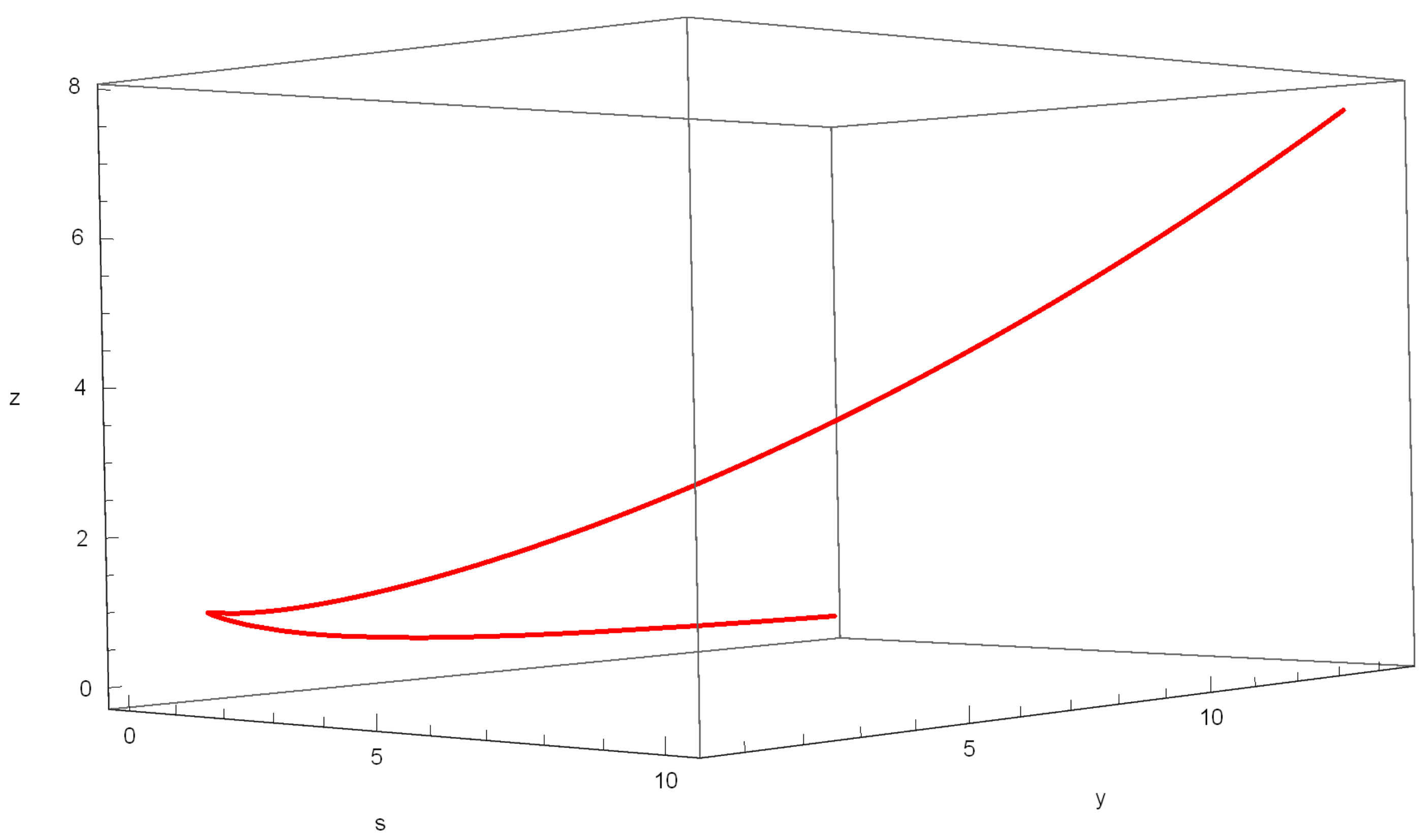
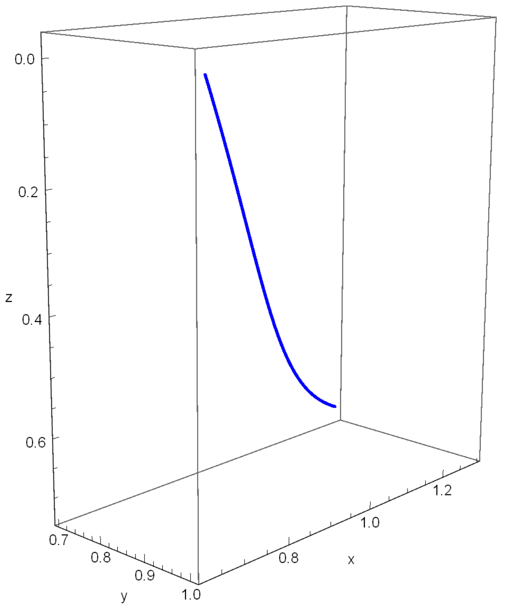
First, consider the curve in the multiplicative equiaffine space, given by multiplicative operations as
or by classical operations as
The curvatures and of this curve are identically equal to or 1. The graph of this curve can be seen in Figure 1.
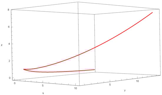
Figure 1.
Graph of Equation (54).
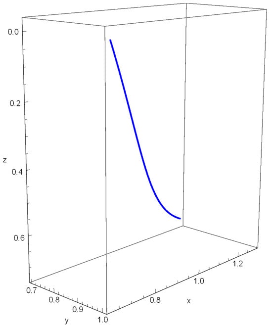
Figure 2.
Graph of Equation (56).
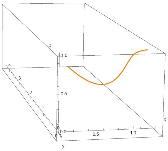
Figure 3.
Graph of Equation (58).
4. Conclusions
This study introduces a comprehensive framework for analyzing curves in multiplicative equiaffine space by integrating concepts from multiplicative calculus and equiaffine differential geometry. Key contributions include the definitions of multiplicative equiaffine arc length, curvature, and torsion, alongside the development of the multiplicative Frenet apparatus and corresponding Frenet equations. Through these tools, the study systematically classifies space curves with constant multiplicative curvature and torsion, providing new insights into the geometric behavior of these curves.
The presented examples demonstrate how multiplicative calculus extends classical geometric concepts, showcasing its potential to generalize and enhance traditional methodologies. These advancements contribute not only to the theoretical development of affine geometry but also highlight potential applications in fields such as physics, engineering, and mathematical modeling, particularly in scenarios involving exponential growth, scaling phenomena, or non-Newtonian frameworks.
Future research could explore the broader applicability of this framework, examining its integration with other geometric and physical systems and its potential to address complex real-world problems.
Author Contributions
Conceptualization, M.O.; Methodology, M.O.; Validation, A.O.O.; Formal analysis, M.O.; Investigation, A.O.O.; Writing—original draft, M.O. and A.O.O.; Writing—review & editing, A.O.O. All authors have read and agreed to the published version of the manuscript.
Funding
This work was not supported by any funding agency.
Data Availability Statement
No new data were created or analyzed in this study. Data sharing is not applicable to this article.
Conflicts of Interest
The authors declare that they have no conflicts of interest.
References
- Volterra, V.; Hostinsky, B. Operations Infinitesimales Lineares; Herman: Paris, France, 1938. [Google Scholar]
- Grossman, M.; Katz, R. Non-Newtonian Calculus, 1st ed.; Lee Press: Pigeon Cove, MA, USA, 1972. [Google Scholar]
- Grossman, M. Bigeometric Calculus: A System with a Scale-Free Derivative; Archimedes Foundation: Rockport, MA, USA, 1983. [Google Scholar]
- Stanley, D. A multiplicative calculus. Primus 1999, 9, 310–326. [Google Scholar] [CrossRef]
- Bashirov, A.; Riza, M. On complex multiplicative differentiation. TWMS Appl. Eng. Math. 2011, 1, 75–85. [Google Scholar]
- Yazici, M.; Selvitopi, H. Numerical methods for the multiplicative partial differential equations. Open Math. 2017, 15, 1344–1350. [Google Scholar] [CrossRef]
- Yalçın, N.; Celik, E. Solution of multiplicative homogeneous linear differential equations with constant exponentials. New Trends Math. Sci. 2018, 6, 58–67. [Google Scholar] [CrossRef]
- Goktas, S.; Kemaloglu, H.; Yilmaz, E. Multiplicative conformable fractional Dirac system. Turk. J. Math. 2022, 46, 973–990. [Google Scholar] [CrossRef]
- Georgiev, S.G.; Zennir, K. Multiplicative Differential Calculus, 1st ed.; Chapman and Hall/CRC: New York, NY, USA, 2022. [Google Scholar]
- Georgiev, S.G. Multiplicative Differential Geometry, 1st ed.; Chapman and Hall/CRC: New York, NY, USA, 2022. [Google Scholar]
- Georgiev, S.G.; Zennir, K.; Boukarou, A. Multiplicative Analytic Geometry, 1st ed.; Chapman and Hall/CRC: New York, NY, USA, 2022. [Google Scholar]
- Nurkan, S.K.; Gurgil, I.; Karacan, M.K. Vector properties of geometric calculus. Math. Methods Appl. Sci. 2023, 46, 17672–17691. [Google Scholar] [CrossRef]
- Has, A.; Yılmaz, B. On non-Newtonian helices in multiplicative Euclidean space E*3. arXiv 2024, arXiv:2403.11282. [Google Scholar] [CrossRef]
- Aydin, M.E.; Has, A.; Yılmaz, B. A non-Newtonian approach in differential geometry of curves: Multiplicative rectifying curves. Bull. Korean Math. Soc. 2024, 61, 849–866. [Google Scholar] [CrossRef]
- Ceyhan, H.; Özdemir, Z.; Gök, İ. Multiplicative generalized tube surfaces with multiplicative quaternions algebra. Math. Methods Appl. Sci. 2024, 47, 9157–9168. [Google Scholar] [CrossRef]
- Broscăţeanu, Ş.C.; Mihai, A.; Olteanu, A. A Note on the Infinitesimal Bending of a Rectifying Curve. Symmetry 2024, 16, 1361. [Google Scholar] [CrossRef]
- Burlacu, A.; Mihai, A. Applications of Differential Geometry of Curves in Roads Design. Rom. J. Transp. Infrastruct. 2023, 12, 1–13. [Google Scholar] [CrossRef]
- Jianu, M.; Achimescu, S.; Dăuş, L.; Mierluş-Mazilu, I.; Mihai, A.; Tudor, D. On a Surface Associated to the Catalan Triangle. Axioms 2022, 11, 685. [Google Scholar] [CrossRef]
- Has, A.; Yılmaz, B.; Yıldırım, H. A non-Newtonian perspective on multiplicative Lorentz-Minkowski space L*3. Math. Methods Appl. Sci. 2024, 47, 13875–13888. [Google Scholar] [CrossRef]
- Özdemir, Z.; Ceyhan, H. Multiplicative hyperbolic split quaternions and generating geometric hyperbolical rotation matrices. Appl. Math. Comput. 2024, 479, 128862. [Google Scholar] [CrossRef]
- Has, A.; Yılmaz, B. A non-Newtonian conics in multiplicative analytic geometry. Turk. J. Math. 2024, 48, 976–994. [Google Scholar] [CrossRef]
- Es, H. Plane kinematics in homothetic multiplicative calculus. J. Univers. Math. 2024, 7, 37–47. [Google Scholar] [CrossRef]
- Has, A.; Yılmaz, B. A non-Newtonian magnetic curves in multiplicative Riemann manifolds. Phys. Scr. 2024, 99, 045238. [Google Scholar] [CrossRef]
- Aydin, M.E.; Has, A.; Yılmaz, B. Multiplicative rectifying submanifolds of multiplicative Euclidean space. Math. Methods Appl. Sci. 2025, 48, 329–339. [Google Scholar] [CrossRef]
- Ceyhan, H.; Özdemir, Z.; Kaya, S.N.; Gürgil, İ. A non-newtonian approach to geometric phase through optic fiber via multiplicative quaternions. Rev. Mex. FíSica 2024, 70, 061301. [Google Scholar] [CrossRef]
- Aydin, M.E.; Mihai, A.; Yokus, A. Applications of fractional calculus in equiaffine geometry: Plane curves with fractional order. Math. Methods Appl. Sci. 2020, 44, 13659–13669. [Google Scholar] [CrossRef]
- Davis, D. Generic affine differential geometry of curves in Rn. Proc. R. Soc. Edinb. 2006, 136, 1195–1205. [Google Scholar] [CrossRef]
- Guggenheimer, H.W. Differential Geometry; McGraw-Hill: New York, NY, USA, 1963. [Google Scholar]
- Nomizu, K.; Sasaki, T. Affine Differential Geometry: Geometry of Affine Immersions; Cambridge Tracts in Mathematics; Cambridge University Press: Cambridge, UK, 1994; Volume 111. [Google Scholar]

Disclaimer/Publisher’s Note: The statements, opinions and data contained in all publications are solely those of the individual author(s) and contributor(s) and not of MDPI and/or the editor(s). MDPI and/or the editor(s) disclaim responsibility for any injury to people or property resulting from any ideas, methods, instructions or products referred to in the content. |
© 2025 by the authors. Licensee MDPI, Basel, Switzerland. This article is an open access article distributed under the terms and conditions of the Creative Commons Attribution (CC BY) license (https://creativecommons.org/licenses/by/4.0/).