DIA-TSK: A Dynamic Incremental Adaptive Takagi–Sugeno–Kang Fuzzy Classifier

Abstract

In order to continuously adapt to dynamic data distributions, existing incremental and online learning methods adopt bagging or boosting structures, in which some sub-classifiers are abandoned when the data distribution varies significantly in the learning process. As such, these ensemble classifiers may fail to reach the global optimum. Furthermore, the training of static sub-classifiers, which are dropped when concept drift emerges, leads to unnecessary computational costs. To solve these issues, this study proposes a novel training method consisting of a single dynamic classifier—named the dynamic incremental adaptive Takagi–Sugeno–Kang fuzzy classifier (DIA-TSK)—which leverages the superior non-linear modeling capabilities and interpretability of the TSK fuzzy system. DIA-TSK utilizes a multi-dimensional incremental learning strategy that is capable of dynamically learning from new data in real time while maintaining global optimal solutions across various online application scenarios. DIA-TSK incorporates two distinct learning paradigms: online learning (O-DIA-TSK) and batch incremental learning (B-DIA-TSK). These modules can work separately or collaborate synergistically to achieve rapid, precise and resource-efficient incremental learning. With the implementation of O-DIA-TSK, we significantly reduce the computational complexity in incremental processes, effectively addressing real-time learning requirements for high-frequency dynamic data streams. Moreover, the novel incremental update mechanism of O-DIA-TSK dynamically adjusts its parameters to ensure progressive optimization, enhancing both real-time performance and learning accuracy. For large-scale data sets, DIA-TSK evolves into B-DIA-TSK, which implements batch updates for multiple samples based on the Woodbury matrix identity. This extension substantially improves computational efficiency and robustness during incremental learning, making it particularly suitable for high-dimensional and complex data sets. Extensive comparative experiments demonstrate that the DIA-TSK approaches significantly outperform existing incremental learning methods across multiple dynamic data sets, exhibiting notable advantages in terms of computational efficiency, classification accuracy and memory management. In the experimental comparison, O-DIA-TSK and B-DIA-TSK reach significant superiority in classification performance with respect to comparative methods, with up to 33.3% and 55.8% reductions in training time, respectively, demonstrating the advantage of DIA-TSK in classification tasks using dynamic data.

1. Introduction

Takagi–Sugeno–Kang (TSK) fuzzy classifiers have achieved unique and superior performance in addressing complex non-linear systems and fuzzy data problems [1,2,3]. This is primarily attributed to their high flexibility and adaptability, enabling them to handle diverse tasks such as prediction, control, classification and optimization. Due to their exceptional global approximation capabilities and remarkable interpretability, TSK fuzzy classifiers have been widely adopted in pattern recognition, data mining, industrial control, medical informatics and other application domains [4]. To meet various practical demands, researchers have developed numerous innovative methods for constructing standalone TSK fuzzy classifiers, such as ANFIS [5,6], GA-based TSK fuzzy classifiers [7], interval type-2 fuzzy systems [8], neuro-fuzzy hybrid TSK classifiers [9] and transfer learning-based TSK classifiers [10]. However, despite these advancements, conventional TSK fuzzy classifiers exhibit inherent limitations when confronted with dynamic incremental changes and large-scale data sets. Specifically, when processing massive, complex and online incremental data, TSK fuzzy classifiers suffer from slow learning speeds, excessive computational resource consumption and sub-optimal performance due to inadequate dynamic parameter updating mechanisms [11].

Researchers have developed three primary incremental learning approaches to adapt classification models to dynamic data sets without complete re-training: sample incremental learning integrates new instances through weight adjustments while mitigating catastrophic forgetting; feature incremental learning dynamically incorporates emerging attributes via dimensional expansion techniques, maintaining cross-feature consistency in evolving environments; and online active learning selects high-informative instances from data streams to optimize the efficiency of annotation and detect concept drift. Specific explanations of these three methods are provided below.

Sample incremental learning emphasizes the efficient integration of new samples into existing models without compromising accuracy or stability. This approach is particularly vital for handling large-scale data, significantly reducing training costs and time. Hu et al. proposed a feature extension and reconstruction method employing scalable feature extractors and optimal transport-based domain mapping, which demonstrated enhanced generalization ability in fault diagnosis applications [12]. However, this approach still relies on relatively static pre-trained feature extractor structures that struggle with truly real-time structural adjustments when confronted with highly dynamic data streams. Hua et al. developed an incremental framework incorporating hybrid data over/down-sampling (HDOD) techniques, achieving performance improvements of 0.47% to 0.71% in gesture classification tasks [13]. Nevertheless, this method addresses concept drift through the use of fixed convolutional network structures and pre-determined sampling strategies, limiting its adaptability to rapidly evolving data distributions. Feng et al. introduced a broad network gradient boosting system with triple incremental capabilities, implemented through an additive architecture optimized via greedy strategies [14]. While avoiding tedious backpropagation, its cascade structure essentially combines static networks whose complexity grows linearly over time, potentially exceeding resource constraints in practical applications. Zheng et al. proposed an incremental learning method for flight dynamics models combining Gaussian process regression with convergence analysis and sample management algorithms [15]; however, this approach still faces computational complexity challenges relating to the use of Gaussian processes on large-scale data sets and difficulties in real-time kernel parameter adjustments in high-dimensional spaces.

Feature incremental learning seeks to extend models through incrementally incorporating new features, enabling their adaptation to shifting data distributions and complexities without the need for full re-training. Despite notable progress in handling large-scale data and fuzzy systems, existing incremental learning methods still face challenges. Primarily, numerous approaches exhibit excessive computational complexity and resource utilization during extensive data updates, rendering them inadequate for real-time online learning applications [16]. Additionally, while weight adjustment and selective sampling strategies enhance accuracy metrics, traditional feature selection algorithms for streaming data often fail to address distribution shifts in non-stationary scenarios, which can significantly degrade their performance when the underlying distributions in data streams change, as has been demonstrated by Wu et al. in their work on incremental Markov boundary learning [17]. Furthermore, existing learning paradigms face critical issues related to sampling bias and representativeness, particularly within dynamic environments characterized by concept drift [18]. Finally, the rigid parameter update mechanisms implemented in many sophisticated systems impede their effective real-time adaptation to extensive data sets [19]. These limitations underscore the imperative for substantial refinements in learning efficiency, generalization capabilities, interpretability frameworks and adaptive mechanisms [20,21].

Online active learning aims to select the most informative instances from continuous data streams for labeling, thereby adapting to evolving data distributions with minimal supervision costs. Despite continuous research progress, existing methods still face critical challenges. According to Guo et al. [22], these techniques struggle to efficiently distinguish outliers from genuine concept drift under limited labeling budgets, resulting in performance degradation. This stems from the model structure’s limited adaptability to dynamic changes, particularly in scenarios characterized by imperfect data. Malialis et al. [23] noted that while existing methods can process individual data arriving in real-time, they still face difficulties in handling non-stationary data while maintaining limited memory occupation. Their proposed ActiSiamese algorithm attempts to address this problem through a novel density-based active learning strategy that evaluates similarity in latent space. Xue et al. [24] demonstrated the limitations of traditional algorithms when processing complex decision scenarios, especially when coordinating resources across different time scales. Conventional methods exhibit high computational complexity, making them unsuitable for real-time applications. Concurrently, in another study, Guo et al. [25] emphasized that existing methods typically assume that all data labels are available in concept drift environments—which is unrealistic in practical applications—causing models to struggle with timely adaptation to distribution changes. Fan et al. [26] further pointed out that traditional methods lack effective incremental learning mechanisms when confronted with continuous unlabeled data chunks and high labeling costs. Their developed two-stage active learning strategy combines diversity and uncertainty queries to enhance the adaptability of models.

The aforementioned existing methods encounter the following challenges:

(1)

The static structures of the existing method have difficulty changing flexibly when facing dynamic data streams. Although some online learning and incremental leaning methods manage to adapt to dynamic data scenarios through assembling static sub-classifiers (which are then dropped when the data distribution alters), they still intrinsically work in a static and not dynamic way.

(2)

Due to their static structure, existing methods can hardly reach the global optimum for the changing dynamic data in real time. Therefore, there inevitably remains a significant margin between the classification performance of these methods and the separability of the data distribution.

(3)

As existing methods utilize a static mechanism, updating their structure may cause unacceptable computational burden in practice, leading these methods to lose their real-time capability (which is widely required in various application scenarios).

In summary, the existing online learning and incremental learning methods cannot keep pace with the drift of dynamic data in real time.

In order to overcome the challenges faced by the existing online learning and incremental learning methods, this study proposes a novel dynamic incremental adaptive TSK fuzzy classifier (DIA-TSK) incorporating two incremental learning strategies: online learning (O-DIA-TSK) and batch incremental learning (B-DIA-TSK). Through synergizing these approaches, DIA-TSK demonstrates superior computational efficiency, flexibility and predictive accuracy in dynamic data environments, particularly for online learning, batch incremental tasks and large-scale data streams. The main contributions of this work are summarized as follows:

(1)

DIA-TSK works through a pure dynamic mechanism, automatically adjusting the model parameters in real time under changing data distributions. This ensures that the classifier consistently maintains optimal performance across evolving data environments.

(2)

DIA-TSK employs a single, dynamically adaptive classifier, instead of the unified frameworks used in existing online learning and incremental learning method implemented with bagging or boosting approaches. This innovative method continuously adjusts the parameters and structure of the classifier in response to new data. The single-classifier architecture enables more efficient computation, faster adaptation to evolving distributions and a stronger theoretical guarantee of optimality.

(3)

DIA-TSK delivers superior performance through its dynamic architecture that continuously optimizes parameters via efficient matrix transformations. This mathematical approach reduces the computational complexity from cubic to quadratic, enabling genuine online incremental learning with minimal overhead. This exceptional efficiency allows for real-time processing of streaming data and immediate adaptation to distribution changes, making DIA-TSK ideal for time-sensitive application environments.

(4)

Extensive experiments demonstrate that DIA-TSK outperforms state-of-the-art online learning and incremental learning methods across multiple dynamic data sets. In both online and batch mode incremental forms, DIA-TSK achieves significant advantages in classification efficiency and prediction accuracy.

The remainder of this paper is organized as follows: Section 2 briefly reviews classical TSK fuzzy classifiers. Section 3 details the proposed DIA-TSK framework, including its two variants and applicable scenarios. Section 4 presents the experimental results, comparing DIA-TSK with baseline methods on 15 benchmark data sets. Conclusions are drawn in Section 5.

2. Zero-Order TSK Fuzzy Classifier

Due to their interoperability and concise structure, zero-order TSK fuzzy classifiers have been the focus of intensive research; therefore, a zero-order TSK fuzzy classifier was adopted as the basis of DIA-TSK. The zero-order TSK fuzzy classifier is an intelligent system based on fuzzy rules, utilizing the principles of fuzzy logic to perform classification on input data. This classifier is composed of a series of fuzzy rules, each corresponding to a specific fuzzy region in the input space. The general form of these fuzzy rules is represented by Equation (1) [27,28]:

$$IF x_1 is A_1^k\wedge x_2 is A_2^k\wedge \cdots \wedge x_d is A_d^k, THEN y^k=a^k,k=1,2,\cdots ,K.$$

(1)

In this expression, $A_j^k$ represents the fuzzy set of the $j$^th feature in the $k$^th fuzzy rule [3], $K$ denotes the total number of fuzzy rules, and $a^k$ is the output value of the $k$^th fuzzy rule. To derive a specific classification result from these fuzzy rules, a process of defuzzification is required. The final output $y$ of the model is calculated using the weighted summation Equation (2) [29]:

$$y=\sum _{k=1}^K {\displaystyle \frac{g^k\left(\mathbf{x}\right)}{{\sum }_{k^{\prime }=1}^K g^{k^{\prime }}}}{a}^k,$$

(2)

where $g^k\left(\mathbf{x}\right)$ is the fuzzy membership function of the sample $\mathbf{x}$ with respect to the $k$^th fuzzy rule, calculated using Equation (3) [30,31]:

$$g^k\left(\mathbf{x}\right)=\prod _{j=1}^d {\psi }_j^k\left(x_j\right),$$

(3)

in which the Gaussian function described in Equation (4) is adopted as the fuzzy member function to capture the fuzzy characteristics of the data and enhance the model’s adaptability [32]:

$${\psi }_j^k\left(x_j\right)=exp\left(-{\displaystyle \frac{1}{2}}{\left({\displaystyle \frac{x_j-m_j^k}{s_j^k}}\right)}^2\right),$$

(4)

where $m_j^k$ and $s_j^k$ represent the center and standard deviation of the Gaussian function, respectively.

We adopt one-hot encoding to represent different categories. In particular, for a data set containing $C$ classes, the label of each class is represented as a binary sequence of length $C$. In the binary sequence for the $c$^th class, only the $c$^th value is 1, while the rest are 0 [29].

Let $\mathbf{X}={\left[x_{nj}\right]}_{N\times d}$ be the training data set matrix, where each row ${\mathbf{x}}_n=\left(x_{n1},x_{n2},\dots ,x_{nd}\right)$ represents the $n$^th training sample; let $\mathbf{Y}={\left[y_{nc}\right]}_{N\times C}$ be the label matrix of the training data set, where ${\mathbf{y}}_n=\left(y_{n1},y_{n2},\dots ,y_{nc}\right)$ is the label vector of the $n$^th sample; and let $\mathbf{M}={\left[m_{kj}\right]}_{K\times d}$ be the fuzzy rule antecedent matrix, where each row $m_k=\left(m_{k1},m_{k2},\dots ,m_{kd}\right)$ represents the antecedent of the $k$^th fuzzy rule. During the training process, the membership of each training sample to each fuzzy rule is computed using Equations (3) and (4), allowing for the construction of the matrix $\mathbf{G}$:

$$\mathbf{G}={\left[{ g}_k\left({\mathbf{x}}_n\right) \right]}_{N\times K}, n=1,2,\dots ,N, k=1,2,\dots ,K,$$

(5)

$${ g}_k\left({\mathbf{x}}_n\right)=\prod _{j=1}^d {\psi }_j^k\left(x_{nj}\right),$$

(6)

$${\psi }_j^k\left(x_{nj}\right)=exp\left(-{\displaystyle \frac{1}{2}}{\left({\displaystyle \frac{x_{nj}-m_j^k}{s_j^k}}\right)}^2\right).$$

(7)

This leads to the following linear system for the fuzzy rule consequent matrix $A={\left[a_{kc}\right]}_{K\times C}$:

$$\mathbf{G}\mathbf{A}=\mathbf{Y}.$$

(8)

As ${\mathbf{G}}^T\mathbf{G}$ is a $K\times K$ positive definite matrix, it is invertible. Therefore, the optimal solution to this equation is given by

$$A={\left({\mathbf{G}}^T\mathbf{G}\right)}^{-1}{\mathbf{G}}^T\mathbf{Y}.$$

(9)

To obtain the output vector corresponding to a test sample x from the trained TSK fuzzy classifier, we compute

$$\mathbf{y}={\left[{ g}_k\left(\mathbf{x}\right) \right]}_{1\times K}\mathbf{A}.$$

(10)

The label of the test sample $\mathbf{x}$ is determined by the category corresponding to the largest element in $\mathbf{y}$.

In order to explain the interpretability of the TSK fuzzy classifier and its associated fuzzy rules t, a set of fuzzy rules in the healthcare context are introduced as follows, in which BP, BS and IL denote “Blood Pressure”, “Blood Sugar” and “Intervention Level”, respectively.

• IF BP is “Normal” AND BS is “Normal”, THEN IL is “No Intervention Required”;
• IF BP is “Normal” AND BS is “Slightly Elevated”, THEN IL is “Mild Intervention”;
• IF BP is “High” AND BS is “Normal”, THEN IL is “Moderate Intervention”;
• IF BP is “High” AND BS is “High”, THEN IL is “Severe Intervention”.

Each fuzzy rule represents a judgment rule or knowledge that determines the level of medical intervention. The semantics “Slightly”, “Normal” and “High” will be, respectively, quantified as 0, 0.5 and 1, and the semantics “No Intervention Required”, “Mild Intervention”, “Moderate Intervention” and “Severe Intervention” will be, respectively, quantified as 0, 1, 2 and 3. Then, the four fuzzy rules can be described as follows:

• IF BP is 0.5 AND BS is 0.5, THEN IL is 0;
• IF BP is 0.5 AND BS is 0, THEN IL is 1;
• IF BP is 1 AND BS is 0.5, THEN IL is 2;
• IF BP is 1 AND BS is 1, THEN IL is 3.

Each sample x input into the TSK fuzzy classifier will generate one fuzzy membership function for each of the fuzzy rules: in this case, $g^1\left(x\right)$, $g^2\left(x\right)$, $g^3\left(x\right)$ and $g^4\left(x\right)$. The output of the TSK fuzzy classifier will be calculated as $y={\sum }_{k=1}^4 a^k{g}^k\left(x\right)$, in which $a^k$ denotes the quantified THEN part of the kth fuzzy rule. The value of y indicates the predicted intervention level of sample x. Thus, it can be seen that the meaning of the data in the working mode of the TSK fuzzy classifier can be understood, which guarantees their interpretability.

However, the problem of how to update the THEN part of the fuzzy rules in real time as the classifier learns new training data remains unsolved.

3. DIA-TSK

In traditional TSK fuzzy classifiers, the addition of new samples is typically limited to statically supplementing new fuzzy rules, which then remain unchanged after supplementation. This approach fails to fully utilize the dynamic information carried by the new samples, resulting in the model’s inability to adapt to new data distributions. Moreover, traditional models often require complete re-training or, at least, computationally expensive partial parameter updates when receiving new data, which significantly reduces the system’s response speed and processing efficiency in applications characterized by large data scales or frequent updates. To address this issue, the proposed incremental TSK fuzzy classifier significantly improves the situation through adopting a dynamic parameter adjustment strategy. This strategy integrates new data directly through efficient computational methods, achieving immediate updating of the consequent parameters. This method not only reduces the demand for computational resources but also significantly shortens the update cycle, enabling the model to quickly adapt to new data inputs, thereby gaining advantages in terms of classification accuracy and computational efficiency in data streams and online scenarios.

This study proposes a novel incremental learning fuzzy classifier, namely, the DIA-TSK. This classifier is specifically designed to adapt to new samples through updating the parameters of existing fuzzy rules, avoiding the need for re-training of the entire model as in traditional methods. The core characteristics of DIA-TSK are its structural flexibility and the efficiency of its update mechanism. This method can learn one or a batch of new samples at a time, or it can eliminate the influence of already-learned abnormal samples from the existing structure. These two different scenarios lead to the definition of the online dynamic incremental adaptive TSK fuzzy classifier (O-DIA-TSK) and the batch dynamic incremental adaptive TSK fuzzy classifier (B-DIA-TSK). In O-DIA-TSK, the model learns only one sample at a time, achieving fine-grained adjustments; meanwhile, in B-DIA-TSK, the model learns multiple samples at once, improving the efficiency of model updates. The consideration of these two scenarios enhances the model’s adaptability and flexibility, enabling it to better cope with dynamic data changes. The advantage of adopting an incremental learning strategy is its ability to efficiently handle dynamically changing data streams, significantly reducing the model re-training costs caused by data updates and enhancing the model’s immediate response capability. Moreover, incremental learning helps to reduce the model’s memory footprint, as it avoids re-learning the entire data set with each update of the data. In summary, DIA-TSK provides a flexible and efficient model with a dynamic real-time update strategy for dynamic data environments utilizing an incremental learning mechanism.

In detail, when a zero-order TSK fuzzy classifier with $K$ fuzzy rules is trained on a data set $X=\{x_n\mid n=1,2,\dots ,N\}$, $N\times K$ fuzzy membership functions are derived; that is, $g_k\left({\mathbf{x}}_n\right),k=1,2,\dots ,K,n=1,2,\dots ,N$. These fuzzy membership functions determine a matrix $\mathbf{G}=\left[g_k\right({\mathbf{x}}_n){]}_{N\times K}$. According to the definition of the TSK fuzzy classifier, as detailed in Section 2, the consequent parameters of the $K$ fuzzy rules can be derived as $\mathbf{A}={\left({\mathbf{G}}^T\mathbf{G}\right)}^{-1}{\mathbf{G}}^T\mathbf{Y}$, in which the calculation of the inverse of ${\mathbf{G}}^T\mathbf{G}$ requires significant computation. If another new data set $X^{\prime }$ consisting of $N^{\prime }$ samples is added to the training data set, some new fuzzy memberships are derived, namely, $g_k\left({\mathbf{x}}_n^{\prime }\right),k=1,2,\dots ,K,n=N+1,N+2,\dots ,{N+N}^{\prime }$. The ${(N+N}^{\prime })\times K$ fuzzy membership functions compose a larger matrix ${\mathbf{G}}^{\mathbf{\prime }}=\left[\begin{array}{c}\mathbf{G}\\ \mathbf{g}\end{array}\right]={\left[\begin{array}{c}{g}_k\left({\mathbf{x}}_n\right)\\ g_k\left({\mathbf{x}}_n^{\prime }\right)\end{array}\right]}_{(N+N^{\prime })\times K}$. For existing training methods of TSK fuzzy classifiers, which work in a static manner, a complete re-training process is needed to derive the consequent parameters of the K fuzzy rules. This process has such a high computational burden that existing TSK fuzzy classifiers cannot operate effectively in real-time. Different from the existing TSK fuzzy classifiers working in a static manner, DIA-TSK derives the optimum of the consequent part matrix $A$’ of the K fuzzy rules subject to $\mathbf{G}\mathbf{\prime }\mathbf{A}=\mathbf{Y}$. In DIA-TSK, G’ is described as the expansion of $\mathbf{G}$—that is, ${\mathbf{G}}^{\prime }=\left[\begin{array}{c}\mathbf{G}\\ \mathbf{g}\end{array}\right]={\left[\begin{array}{c}{g}_k\left({\mathbf{x}}_n\right)\\ g_k\left({\mathbf{x}}_n^{\prime }\right)\end{array}\right]}_{(N+N^{\prime })\times K}$, in which $g=\left[g_k\right({\mathbf{x}}_n^{\prime }){]}_{N^{\prime }\times K}$—and the expected new consequent part matrix ${\mathbf{A}}^{\prime }$ is calculated as ${\mathbf{A}}^{\prime }=\mathbf{A}+\Delta \mathbf{A}$. With the existing ${\left({\mathbf{G}}^T\mathbf{G}\right)}^{-1}$, DIA-TSK succeeds in deriving $\Delta \mathbf{A}$ analytically with low computational cost.

Take the trained TSK fuzzy classifier for the prediction of medical intervention level on an input sample given at the end of Section 2 as an example. After DIA-TSK processing, the fuzzy rules may be adjusted as follows:

• IF BP is 0.5 AND BS is 0.5, THEN IL is 0.1;
• IF BP is 0.5 AND BS is 0, THEN IL is 0.9;
• IF BP is 1 AND BS is 0.5, THEN IL is 2.2;
• IF BP is 1 AND BS is 1, THEN IL is 3.0.

These are the optimal rules to describe the new training data set.

3.1. Online Dynamic Incremental Adaptive TSK Fuzzy Classifier (O-DIA-TSK)

The O-DIA-TSK classifier adopts an online dynamic incremental learning strategy to learn new individual samples in real time. In the initial training process, O-DIA-TSK uses the initial training data set $X_0$ to train a TSK fuzzy classifier ${TSK}_0$ containing $K$ fuzzy rules, obtaining the antecedent matrix ${\mathbf{G}}_0={\left[{ g}_k\left({\mathbf{x}}_n\right) \right]}_{N\times K}$, ${\left({\mathbf{G}}_0^T{\mathbf{G}}_0\right)}^{-1}$ and the fuzzy rule consequent matrix ${\mathbf{A}}_0$. Using Equations (11) and (12), the membership function vectors ${\underset{\_}{\mathbf{g}}}_1={\left[{ g}_k\left({\underset{\_}{\mathbf{x}}}_1\right) \right]}_{1\times K}$ for the $K$ fuzzy rules are calculated for a new training sample $\left({\underset{\_}{\mathbf{x}}}_1 {\underset{\_}{\mathbf{y}}}_1\right)$ as follows:

$${ g}_k\left({\underset{\_}{\mathbf{x}}}_1\right)=\prod _{j=1}^d {\psi }_j^k\left({\underset{\_}{x}}_{nj}\right),$$

(11)

$${\psi }_j^k\left({\underset{\_}{x}}_{nj}\right)=exp\left(-{\displaystyle \frac{1}{2}}{\left({\displaystyle \frac{{\underset{\_}{x}}_{nj}-m_j^k}{s_j^k}}\right)}^2\right).$$

(12)

Then, the optimal TSK fuzzy classifier ${TSK}_1$, which shares the same fuzzy rule antecedents as ${TSK}_0$, is trained using the extended training data set ${\mathbf{X}}_1={\mathbf{X}}_0\cup \left\{{\underset{\_}{\mathbf{x}}}_1\right\}$. The consequent matrix ${\mathbf{A}}_1$ is obtained as the least-squares solution of Equation (13):

$${\mathbf{G}}_1{\mathbf{A}}_1={\mathbf{Y}}_1.$$

(13)

where

$${\mathbf{G}}_1={\left[{\mathbf{G}}_0;{\underset{\_}{\mathbf{g}}}_1\right]}_{(N+1)\times K}, {\mathbf{Y}}_1={\left[{\mathbf{Y}}_0;{\underset{\_}{\mathbf{y}}}_1\right]}_{(N+1)\times C}.$$

(14)

In order to reduce the computational complexity by leveraging the fuzzy rule consequents of the already trained TSK fuzzy classifier, let

$${\mathbf{A}}_1={\mathbf{A}}_0+\Delta {\mathbf{A}}_1.$$

(15)

Thus, Equation (13) can be further represented as

$$\left[\begin{array}{c}{\mathbf{G}}_0\\ {\underset{\_}{\mathbf{g}}}_1\end{array}\right]\left({\mathbf{A}}_0+\Delta {\mathbf{A}}_1\right)=\left[\begin{array}{c}{\mathbf{Y}}_0\\ {\underset{\_}{\mathbf{y}}}_1\end{array}\right].$$

(16)

The optimal solution of this equation is

$$\begin{array}{ll}\Delta {\mathbf{A}}_1& =({{\mathbf{G}}_1^T{\mathbf{G}}_1)}^{-1}{\mathbf{G}}_1^T\left({\mathbf{Y}}_1-{\mathbf{G}}_1{\mathbf{A}}_0\right)\\ & =({{\mathbf{G}}_1^T{\mathbf{G}}_1)}^{-1}{\mathbf{G}}_1^T\left({\mathbf{Y}}_1-{\mathbf{G}}_1{\mathbf{A}}_0\right)\\ & =({{\mathbf{G}}_1^T{\mathbf{G}}_1)}^{-1}\left[{\mathbf{G}}_0^T{\mathbf{Y}}_1-{\mathbf{G}}_0^T{\mathbf{G}}_0{\mathbf{A}}_0+{\mathbf{g}}_1^T\left({\underset{\_}{\mathbf{y}}}_1-{\underset{\_}{\mathbf{g}}}_1{\mathbf{A}}_0\right)\right].\end{array}$$

(17)

In Equation (17) above, ${\mathbf{G}}_0^T{\mathbf{Y}}_1$ and ${\mathbf{G}}_0^T{\mathbf{G}}_0$ have already been computed during the training of ${TSK}_0$ and the computational cost of the vector ${\mathbf{g}}_1^T\left({\underset{\_}{\mathbf{y}}}_1-{\underset{\_}{\mathbf{g}}}_1{\mathbf{A}}_0\right)$ is minimal. As the number of training samples increases, the computation of $({{\mathbf{G}}_1^T{\mathbf{G}}_1)}^{-1}$ grows cubically. To reduce the computational cost, the Sherman–Morrison formula is applied to transform $({{\mathbf{G}}_1^T{\mathbf{G}}_1)}^{-1}$, as shown in Equation (18), which simplifies its computation:

$$({{\mathbf{G}}_1^T{\mathbf{G}}_1)}^{-1}={\left({\mathbf{G}}_0^T{\mathbf{G}}_0\right)}^{-1}-{\displaystyle \frac{{\left({\mathbf{G}}_0^T{\mathbf{G}}_0\right)}^{-1}{\mathbf{g}}_1^T{\underset{\_}{\mathbf{g}}}_1{\left({\mathbf{G}}_0^T{\mathbf{G}}_0\right)}^{-1}}{1+{\underset{\_}{\mathbf{g}}}_1{\left({\mathbf{G}}_0^T{\mathbf{G}}_0\right)}^{-1}{\mathbf{g}}_1^T}}.$$

(18)

Notably, the most computationally expensive term ${\left({\mathbf{G}}_0^T{\mathbf{G}}_0\right)}^{-1}$ has already been computed during the training of ${TSK}_0$.

In general, for the t^th newly added training sample, the classifier ${TSK}_t$ is trained. The membership for the new training sample $\left({\underset{\_}{\mathbf{x}}}_t,{\underset{\_}{\mathbf{y}}}_t\right)$ with respect to the $K$ fuzzy rules is calculated as a row vector of membership functions, denoted as ${\underset{\_}{\mathbf{g}}}_t={\left[g_k\left({\underset{\_}{\mathbf{x}}}_t\right)\right]}_{1\times K}$, using Equations (19) and (20):

$${ g}_k\left({\underset{\_}{\mathbf{x}}}_t\right)=\prod _{j=1}^d {\psi }_j^k\left({\underset{\_}{x}}_{tj}\right),$$

(19)

$${\psi }_j^k\left({\underset{\_}{x}}_{tj}\right)=exp\left(-{\displaystyle \frac{1}{2}}{\left({\displaystyle \frac{{\underset{\_}{x}}_{tj}-m_j^k}{s_j^k}}\right)}^2\right).$$

(20)

Thus, using the updated training data set ${\mathbf{X}}_t={\mathbf{X}}_{t-1}\cup \left\{{\underset{\_}{\mathbf{x}}}_t\right\}$, the optimal TSK fuzzy classifier ${TSK}_t$ that shares the same fuzzy rules as ${TSK}_0,{TSK}_1,\cdots ,{TSK}_{t-1}$ is determined by solving the least-squares problem for the consequent matrix A_t based on the following equation. Then, the consequent matrix A_t is obtained as the least-squares solution of Equation (21):

$${\mathbf{G}}_t{\mathbf{A}}_t={\mathbf{Y}}_t,$$

(21)

where

$${\mathbf{G}}_t={\left[{\mathbf{G}}_{t-1};{\underset{\_}{\mathbf{g}}}_t\right]}_{(N+1)\times K}, {\mathbf{Y}}_t={\left[{\mathbf{Y}}_{t-1};{\underset{\_}{\mathbf{y}}}_t\right]}_{(N+1)\times C}.$$

(22)

Let

$${\mathbf{A}}_t={\mathbf{A}}_{t-1}+\Delta {\mathbf{A}}_t.$$

(23)

Thus, Equation (18) can be further represented as

$${\mathbf{G}}_t\left({\mathbf{A}}_{t-1}+\Delta {\mathbf{A}}_t\right)={\mathbf{Y}}_t.$$

(24)

The optimal solution of this equation is

$$\Delta {\mathbf{A}}_t=({{\mathbf{G}}_t^T{\mathbf{G}}_t)}^{-1}\left[{\mathbf{G}}_{t-1}^T{\mathbf{Y}}_t-{\mathbf{G}}_{t-1}^T{\mathbf{G}}_{t-1}{\mathbf{A}}_{t-1}+{\mathbf{g}}_t^T\left({\underset{\_}{\mathbf{y}}}_t-{\underset{\_}{\mathbf{g}}}_t{\mathbf{A}}_{t-1}\right)\right].$$

(25)

As the O-DIA-TSK method produces a standard TSK fuzzy classifier, the testing process is the same as that for a regular TSK fuzzy classifier. Specifically, when the testing data set X is input into TSK_t, the output is given by Equation (26):

$${\tilde{\mathbf{Y}}}_t={\tilde{\mathbf{G}}}_t{\mathbf{A}}_t,$$

(26)

where ${\tilde{\mathbf{G}}}_t={\left[{\mathbf{g}}_k\left({\mathbf{x}}_n\right)\right]}_{N\times K}$. The class of each test sample is determined by the column of the row in ${\tilde{\mathbf{Y}}}_t$ that has the maximum element.

The proposed O-DIA-TSK method dynamically increases ${\mathbf{G}}_t^T{\mathbf{G}}_t$ with one row and one column by adding the membership functions for the new training sample to the fuzzy rules, thus effectively reducing the time complexity. It is applicable in two typical scenarios: first, when new data streams continuously add new samples for online learning, and second, when the data complexity changes, dynamically adding individual samples to improve the prediction accuracy, thereby adapting to more complex and dynamic data environments.

The specific training process of the model is shown in Algorithm 1.

Algorithm 1: The training process of the O-DIA-TSK fuzzy classifier.

Input  Training set $\mathbf{D}=\left\{{\mathbf{x}}_1,{\mathbf{x}}_2,\dots ,{\mathbf{x}}_N\right\}$, where ${\mathbf{x}}_n\in {\mathbb{R}}^d$, $N$ denotes the number of training samples and $d$ is the dimension of the samples. Corresponding class labels $\mathbf{Y}=[{\mathbf{y}}_1,{\mathbf{y}}_2,\dots ,{\mathbf{y}}_N{]}^T$, where ${\mathbf{y}}_n$ is represented as a one-hot binary encoded vector. The initial number of fuzzy rules $K_0$ for the TSK classifier, width $s$ of the Gaussian membership function and the number of incremental learning rounds $T$. Output  Consequent parameters ${\mathbf{A}}_0=\left[{\mathit{a}}_1;{\mathit{a}}_2;\dots ;{\mathit{a}}_{K_0}\right]$ of the initial classifier. Predicted ${\overline{\mathbf{Y}}}_T$ and updated consequent parameters ${\mathbf{A}}_T=$$[{\mathit{a}}_1^T;{\mathit{a}}_2^T;\dots ;{\mathit{a}}_{K_0}^T$] after $T$ rounds of incremental learning. Initial TSK Classifier Training Process Step 1. Compute Gaussian membership functions using the input data $\mathbf{X}=[{\mathbf{x}}_1,{\mathbf{x}}_2,\dots ,{\mathbf{x}}_N]$

$${\psi }_j^k\left({\underset{\_}{x}}_{nj}\right)=exp\left(-{\displaystyle \frac{1}{2}}{\left({\displaystyle \frac{{\underset{\_}{x}}_{nj}-m_j^k}{s_j^k}}\right)}^2\right),$$ (27)

where $x_j$ is the $j$th feature of sample x, $m_j^k\in$ {0, 0.25, 0.5, 0.75, 1} and $k=1,2,\dots ,K_0$. The membership of each sample for all initial fuzzy rules is calculated as

$$g\left({\mathbf{x}}_n\right)={\displaystyle \sum _{k=1}^K} {\displaystyle \frac{{\prod }_{j=1}^d {\mu }_{kj}\left(x_{nj}\right)}{{\sum }_{k^{\prime }=1}^K {\prod }_{j=1}^d {\mu }_{k^{\prime }j}\left(x_j\right)}}.$$ (28)

Construct the antecedent matrix of the initial $K_0$ fuzzy rules

$${\mathbf{G}}_0={\left[{\mathbf{g}}_{k_0}\left({\mathbf{x}}_n\right)\right]}_{N\times K_0},$$ (29)

forming an overdetermined linear system for the consequent parameter matrix ${\mathbf{A}}_0$

$${\mathbf{G}}_0{\mathbf{A}}_0=\mathbf{Y}.$$ (30)

Step 2. Obtain the analytical solution for the consequent parameters [24]

$${\mathbf{A}}_0={\left({{\mathbf{G}}_0}^{{\rm T}}{\mathbf{G}}_0\right)}^{-1}{{\mathbf{G}}_0}^{{\rm T}}\mathbf{Y}.$$ (31)

Step 3. Compute the output of the classifier as

$${\overline{\mathbf{Y}}}_0={\mathbf{G}}_0 {\mathbf{A}}_0.$$ (32)

Output ${\overline{\mathbf{Y}}}_0$ and ${\mathbf{A}}_0$. Incremental Training Process Step 4. for $t=1$ to $T$do           Step 4.1. Generate the membership row vector ${\underset{\_}{\mathbf{g}}}_t=\left[{\mathbf{g}}_k\right({\underset{\_}{\mathbf{x}}}_t){]}_{1\times K}$ for the new sample, $({\underset{\_}{\mathbf{x}}}_t,{\underset{\_}{y}}_t)$, following Step 1.           Step 4.2. Update the antecedent matrix ${\mathbf{G}}_t={\left[\begin{array}{c}{\mathbf{G}}_{t-1}\\ {\underset{\_}{\mathbf{g}}}_t\end{array}\right]}_{(N+t)\times K}.$           Step 4.3. Compute the adjustment to the consequent parameters

$$\Delta {\mathbf{A}}_t=({{\mathbf{G}}_t^T{\mathbf{G}}_t)}^{-1}\left[{\mathbf{G}}_{t-1}^T{\mathbf{Y}}_t-{\mathbf{G}}_{t-1}^T{\mathbf{G}}_{t-1}{\mathbf{A}}_{t-1}+{\mathbf{g}}_t^T\left({\underset{\_}{\mathbf{y}}}_t-{\underset{\_}{\mathbf{g}}}_t{\mathbf{A}}_{t-1}\right)\right].$$ (33)

Step 4.4. Update the consequent parameters

$${\mathbf{A}}_t={\mathbf{A}}_{t-1}+\Delta {\mathbf{A}}_t.$$ (34)

Step 5. After $T$ iterations, compute the final predictions

$${\overline{\mathbf{Y}}}_T={\mathbf{G}}_T{\mathbf{a}}_T.$$ (35)

Output ${\overline{\mathbf{Y}}}_T$ and ${\mathbf{A}}_T$. Main Procedure Step 6. Train the initial TSK fuzzy classifier and output G0 and A0. Step 7. If the training accuracy is unsatisfactory, invoke the incremental training process to output           ${\overline{\mathbf{Y}}}_T$ and ${\mathbf{A}}_T$.

3.2. Batch Dynamic Incremental Adaptive TSK Fuzzy Classifier (B-DIA-TSK)

In the context of new data arriving in batch mode, DIA-TSK naturally evolves into the B-DIA-TSK. The primary advantages of this approach are as follows. First, the batch update algorithm processes a group of new samples simultaneously, significantly reducing the total computational time. Compared with O-DIA-TSK, which is updated with single samples, batch updating more efficiently utilizes matrix parallel computation, enhancing the overall processing speed. Specifically, B-DIA-TSK employs the Woodbury matrix identity to optimize the computation of the pseudo-inverse matrix of the fuzzy rule membership matrix in the data set, which leads to a reduction in computational complexity, making it independent of the number of new samples. Second, by processing multiple samples in a single computation, the algorithm is able to perform multiple update steps simultaneously, reducing the potential for error propagation and accumulation, thus helping to maintain the stability of the model. Moreover, the batch updating algorithm is more efficient in utilizing memory and computational resources.

Initially, during the training process, B-DIA-TSK uses the initial training data set $R^0=\left\{\left(x_n,y_n \right):1\le n\le N\right\}$ to train the TSK fuzzy classifier ${TSK}_0$, which contains $K$ fuzzy rules. This results in the membership matrix ${\mathbf{G}}_0={\left[{\mathbf{g}}_k\left({\mathbf{x}}_n\right)\right]}_{N\times K}$ and the fuzzy rule consequent matrix $A_0$. Using Equations (36) and (37), the fuzzy rule membership matrix for the new training set ${\underset{\_}{R}}^1=\left\{\left({\underset{\_}{\mathbf{x}}}_n^1,{\underset{\_}{\mathbf{y}}}_n^1 \right):1\le n\le N^1\right\}$ is computed using

$${ g}_k\left({\underset{\_}{\mathbf{x}}}_n^1\right)=\prod _{j=1}^d {\psi }_j^k\left({\underset{\_}{x}}_{nj}^1\right),$$

(36)

$${\psi }_j^k\left({\underset{\_}{x}}_{nj}^1\right)=exp\left(-{\displaystyle \frac{1}{2}}{\left({\displaystyle \frac{{\underset{\_}{x}}_{nj}^1-m_j^k}{s_j^k}}\right)}^2\right).$$

(37)

The optimal TSK fuzzy classifier ${TSK}_1$ is trained using the extended training data set $R_1=R_0\cup {\underset{\_}{R}}_1$, while sharing the same fuzzy rule antecedents as ${TSK}_0$. Its consequent matrix ${\mathbf{A}}_1$ is solved as follows.

$${\mathbf{G}}_1{\mathbf{A}}_1={\mathbf{Y}}_1,$$

(38)

where

$${\mathbf{G}}_1={\left[{\mathbf{G}}_0;{\underset{\_}{\mathbf{G}}}_1\right]}_{(N+N_1)\times K}, {\mathbf{Y}}_1={\left[{\mathbf{Y}}_0;{\underset{\_}{\mathbf{Y}}}_1\right]}_{(N+N_1)\times C}.$$

(39)

To reduce the computational complexity of this process using the fuzzy rule consequents of the previously trained TSK classifier, we define

$${\mathbf{A}}_1={\mathbf{A}}_0+\Delta {\mathbf{A}}_1.$$

(40)

Thus, Equation (38) can be rewritten as

$$\left[\begin{array}{c}{\mathbf{G}}_0\\ {\underset{\_}{\mathbf{G}}}_1\end{array}\right]\left({\mathbf{A}}_0+\Delta {\mathbf{A}}_1\right)=\left[\begin{array}{c}{\mathbf{Y}}_0\\ {\mathbf{Y}}_1\end{array}\right].$$

(41)

The optimal solution to this equation is

$$\Delta {\mathbf{A}}_1={\left({\mathbf{G}}_1^T{\mathbf{G}}_1\right)}^{-1}{\mathbf{G}}_1^T\left({\mathbf{Y}}_1-{\mathbf{G}}_1{\mathbf{A}}_0\right).$$

(42)

Equation (42) can be expanded as shown in Equation (43):

$$\begin{array}{ll}\Delta {\mathbf{A}}_1& =({{\mathbf{G}}_1^{\mathit{T}}{\mathbf{G}}_1)}^{-1}{\mathbf{G}}_1^{\mathit{T}}\left({\mathbf{Y}}_1-{\mathbf{G}}_1{\mathbf{A}}_0\right)\\ & =({{\mathbf{G}}_1^{\mathit{T}}{\mathbf{G}}_1)}^{-1}{\mathbf{G}}_1^{\mathit{T}}\left({\mathbf{Y}}_1-{\mathbf{G}}_1{\mathbf{A}}_0\right)\\ & =({{\mathbf{G}}_1^T{\mathbf{G}}_1)}^{-1}\left[{\mathbf{G}}_0^T{\mathbf{Y}}_1-{\mathbf{G}}_0^T{\mathbf{G}}_0{\mathbf{A}}_0+{\underset{\_}{\mathbf{G}}}_1^T\left({\underset{\_}{\mathbf{Y}}}_1-{\underset{\_}{\mathbf{G}}}_1{\mathbf{A}}_0\right)\right].\end{array}$$

(43)

In Equation (43), ${\mathbf{G}}_0^T{\mathbf{Y}}_1$ and ${\mathbf{G}}_0^T{\mathbf{G}}_0$ were computed during the training of ${TSK}_0$. As the number of new samples is relatively small, the matrix ${\underset{\_}{\mathbf{G}}}_T^T\left({\underset{\_}{\mathbf{Y}}}_1-{\underset{\_}{\mathbf{G}}}_1{A}_0\right)$ has a small computational cost. As the number of new samples increases, the computation of $({{\mathbf{G}}_1^T{\mathbf{G}}_1)}^{-1}$ grows cubically. Through applying the Woodbury matrix identity, we can express $({{\mathbf{G}}_1^T{\mathbf{G}}_1)}^{-1}$ as in Equation (44):

$$\begin{array}{c}({{\mathbf{G}}_1^T{\mathbf{G}}_1)}^{-1}=({\mathbf{G}}_0^T{\mathbf{G}}_0+{\underset{\_}{\mathbf{G}}}_1^T{\underset{\_}{\mathbf{G}}}_1{)}^{-1}\\ =({\mathbf{G}}_0^T{\mathbf{G}}_0{)}^{-1}-({\mathbf{G}}_0^T{\mathbf{G}}_0{)}^{-1}{\underset{\_}{\mathbf{G}}}_1^T(\mathbf{I}+{\underset{\_}{\mathbf{G}}}_1({\mathbf{G}}_0^T{\mathbf{G}}_0{)}^{-1}{\underset{\_}{\mathbf{G}}}_1^T{)}^{-1}{\underset{\_}{\mathbf{G}}}_1({\mathbf{G}}_0^T{\mathbf{G}}_0{)}^{-1}.\end{array}$$

(44)

The most computationally intensive term, $({\mathbf{G}}_0^T{\mathbf{G}}_0{)}^{-1}$, is already available from the training of ${TSK}_0$.

In general, for the $t$^th batch of newly added training data, the classifier ${TSK}_T$ is trained. Using Equations (45) and (46), the membership matrix ${\underset{\_}{\mathbf{G}}}_T={\left[{\mathbf{g}}_k\left({\mathbf{x}}_n^T\right)\right]}_{N^T\times K}$ for each sample in the new training set ${\underset{\_}{R}}^T=\left\{\left({\underset{\_}{\mathbf{x}}}_n^T,{\underset{\_}{\mathbf{y}}}_n^T \right):1\le n\le N^T\right\}$ with respect to the $K$ fuzzy rules is calculated.

$${ g}_k\left({\underset{\_}{\mathbf{x}}}_n^T\right)=\prod _{j=1}^d {\psi }_j^k\left({\underset{\_}{x}}_{nj}^T\right),$$

(45)

$${\psi }_j^k\left({\underset{\_}{x}}_{nj}^T\right)=exp\left(-{\displaystyle \frac{1}{2}}{\left({\displaystyle \frac{{\underset{\_}{x}}_{nj}^T-m_j^k}{s_j^k}}\right)}^2\right).$$

(46)

The optimal TSK fuzzy classifier ${TSK}_T$, which shares the same fuzzy rule antecedents as ${TSK}_0,{TSK}_1,\dots ,{TSK}_{T-1}$, is trained using the extended data set $R_T$. The consequent matrix ${\mathbf{A}}_T$ can be derived by solving the following linear equations in Equation (47).

$${\mathbf{G}}_T{\mathbf{A}}_T={\mathbf{Y}}_T,$$

(47)

where

$${\mathbf{G}}_T={\left[{\mathbf{G}}_{T-1};{\underset{\_}{\mathbf{G}}}_T\right]}_{(N+{\sum }_{t=1}^T N_t)\times K}, {\mathbf{Y}}_T={\left[{\mathbf{Y}}_{T-1};{\underset{\_}{\mathbf{Y}}}_T\right]}_{(N+{\sum }_{t=1}^T N_t)\times C}.$$

(48)

We define ${\mathbf{A}}_T={\mathbf{A}}_{T-1}+\Delta {\mathbf{A}}_T$, such that Equation (47) becomes

$${\mathbf{G}}_T\left({\mathbf{A}}_{T-1}+\Delta {\mathbf{A}}_T\right)={\mathbf{Y}}_T.$$

(49)

The optimal solution to Equation (49) is

$$\Delta {\mathbf{A}}_T=({{\mathbf{G}}_T^T{\mathbf{G}}_T)}^{-1}\left[{\mathbf{G}}_{T-1}^T{\mathbf{Y}}_T-{\mathbf{G}}_{T-1}^T{\mathbf{G}}_{T-1}{\mathbf{A}}_{T-1}+{\underset{\_}{\mathbf{G}}}_T^T\left({\underset{\_}{\mathbf{Y}}}_T-{\underset{\_}{\mathbf{G}}}_T{\mathbf{A}}_{T-1}\right)\right],$$

(50)

where

$$\begin{array}{cc}\hfill ({{\mathbf{G}}_T^T{\mathbf{G}}_T)}^{-1}& =({\mathbf{G}}_{T-1}^T{\mathbf{G}}_{T-1}{)}^{-1}-({\mathbf{G}}_{T-1}^T{\mathbf{G}}_{T-1}{)}^{-1}{\underset{\_}{\mathbf{G}}}_T^T(I\hfill \\ & +{\underset{\_}{\mathbf{G}}}_T\left({\mathbf{G}}_{T-1}^T{\mathbf{G}}_{T-1}{)}^{-1}{\underset{\_}{\mathbf{G}}}_T^T{)}^{-1}{\underset{\_}{\mathbf{G}}}_T\right({\mathbf{G}}_{T-1}^T{\mathbf{G}}_{T-1}{)}^{-1}.\hfill \end{array}$$

(51)

As B-DIA-TSK produces a standard TSK fuzzy classifier, the testing process follows the same procedure as for any ordinary TSK fuzzy classifier. The testing data set $X$ is input into ${TSK}_T$, producing the output $\tilde{\mathbf{Y}}$ as follows:

$$\tilde{\mathbf{Y}}={\tilde{\mathbf{G}}}_T{\mathbf{A}}_T,$$

(52)

where ${\tilde{\mathbf{G}}}_T={\left[{\mathbf{g}}_k\left({\mathbf{x}}_n^v\right) \right]}_{N\times K}$ is the membership matrix for the testing samples with respect to the fuzzy rules and ${\mathbf{x}}_n^v$ is a testing sample. The class of the testing sample corresponds to the column with the maximum value in each row of ${\tilde{\mathbf{Y}}}_T$.

Algorithm 2 describes the B-DIA-TSK training process.

Algorithm 2: The training process of the B-DIA-TSK fuzzy classifier.

Input  Training set $\mathbf{D}=\left\{{\mathbf{x}}_1,{\mathbf{x}}_2,\dots ,{\mathbf{x}}_N\right\}$, where ${\mathbf{x}}_n\in {\mathbb{R}}^d$, $N$ denotes the number of training samples and $d$ is the dimension of the samples. Corresponding class labels $\mathbf{Y}=[{\mathbf{y}}_1,{\mathbf{y}}_2,\dots ,{\mathbf{y}}_N{]}^T$, where ${\mathbf{y}}_n$ is represented as a one-hot binary encoded vector. The initial number of fuzzy rules $K_0$ for the TSK classifier, width $s$ of the Gaussian membership function and the number of incremental learning rounds $T$. Output  Consequent parameters ${\mathbf{A}}_0=\left[{\mathit{a}}_1;{\mathit{a}}_2;\dots ;{\mathit{a}}_{K_0}\right]$ of the initial classifier. Predicted ${\overline{\mathbf{Y}}}_T$ and updated consequent parameters ${\mathbf{A}}_T=$$[{\mathit{a}}_1^T;{\mathit{a}}_2^T;\dots ;{\mathit{a}}_{K_0}^T$] after $T$ rounds of incremental learning. Initial TSK Classifier Training Process Step 1. Compute Gaussian membership functions using the input data $\mathbf{X}=\left[{\mathbf{x}}_1,{\mathbf{x}}_2,\dots ,{\mathbf{x}}_N\right]$:

$${\psi }_j^k\left(x_j\right)=exp\left(-{\displaystyle \frac{1}{2}}{\left({\displaystyle \frac{x_j-m_j^k}{s_j^k}}\right)}^2\right),$$ (53)

where $x_j$ is the $j$th feature of the sample, $m_j^k\in$ {0, 0.25, 0.5, 0.75, 1} and $k=1,2,\dots ,K_0$. The membership of each sample under all initial fuzzy rules is calculated as

$$g\left({\mathbf{x}}_n\right)={\displaystyle \sum _{k=1}^K} {\displaystyle \frac{{\prod }_{j=1}^d {\mu }_{kj}\left(x_{nj}\right)}{{\sum }_{k^{\prime }=1}^K {\prod }_{j=1}^d {\mu }_{k^{\prime }j}\left(x_j\right)}}.$$ (54)

This yields the antecedent matrix of the initial $K_0$ fuzzy rules

$${\mathbf{G}}_0={\left[{\mathbf{g}}_{k_0}\left({\mathbf{x}}_n\right)\right]}_{N\times K_0}.$$ (55)

forming an overdetermined linear system for the consequent parameters ${\mathbf{A}}_0$

$${\mathbf{G}}_0{\mathbf{A}}_0=\mathbf{Y}.$$ (56)

Step 2. Obtain the analytical solution for the consequent parameters [24]

$${\mathbf{A}}_0={\left({\mathbf{G}}_0^T{\mathbf{G}}_0\right)}^{-1}{\mathbf{G}}_0^T\mathbf{Y}.$$ (57)

Step 3. Predict using the obtained parameters

$${\overline{\mathbf{Y}}}_0={\mathbf{G}}_0 {\mathbf{A}}_{0.}$$ (58)

Output ${\overline{\mathbf{Y}}}_0$ and ${\mathbf{A}}_0$. Incremental Training Process Step 4. for $t=1$ to $T$do           Step 4.1. For each sample in the new training set ${\underset{\_}{R}}^1=\left\{\right({\underset{\_}{\mathbf{x}}}_n^1,{\underset{\_}{\mathbf{y}}}_n^1):1\le n\le N^1\}$, the membership for each fuzzy rule is calculated, resulting in the fuzzy rule membership matrix ${\mathbf{G}}_1=\left[{\mathbf{g}}_k\right({\underset{\_}{\mathbf{x}}}_n^1){]}_{N_1\times K}$.           Step 4.2. Update the total fuzzy rule premise matrix after this round of incremental learning:

$${\mathbf{G}}_T=[{\mathbf{G}}_{T-1};{\mathbf{G}}_T{]}_{\left(N+{\sum }_{t=1}^T N_t\right)\times K.}$$ (59)

Step 4.3. With the learning from the current round of incremental data, compute the change in the consequent parameters of the previous fuzzy rules and the addition of new fuzzy rules

$$\Delta {\mathbf{A}}_T=({{\mathbf{G}}_T^T{\mathbf{G}}_T)}^{-1}\left[{\mathbf{G}}_{T-1}^T{\mathbf{Y}}_T-{\mathbf{G}}_{T-1}^T{\mathbf{G}}_{T-1}{\mathbf{A}}_{T-1}+{\underset{\_}{\mathbf{G}}}_T^T\left({\underset{\_}{\mathbf{Y}}}_T-{\underset{\_}{\mathbf{G}}}_T{\mathbf{A}}_{T-1}\right)\right].$$ (60)

where the term $({\mathbf{G}}_T^T{\mathbf{G}}_T{)}^{-1}$ is computed recursively as

$({{\mathbf{G}}_T^T{\mathbf{G}}_T)}^{-1}=({\mathbf{G}}_{T-1}^T{\mathbf{G}}_{T-1}{)}^{-1}-\left({\mathbf{G}}_{T-1}^T{\mathbf{G}}_{T-1}{)}^{-1}{\underset{\_}{\mathbf{G}}}_T^T\right(\mathbf{I}+{\underset{\_}{\mathbf{G}}}_T\left({\mathbf{G}}_{T-1}^T{\mathbf{G}}_{T-1}{)}^{-1}{\underset{\_}{\mathbf{G}}}_T^T{)}^{-1}{\underset{\_}{\mathbf{G}}}_T\right({\mathbf{G}}_{T-1}^T{\mathbf{G}}_{T-1}{)}^{-1}.$

Step 4.4 The consequent parameters of the fuzzy rules are updated for the current round:

$${\mathbf{A}}_t={\mathbf{A}}_{t-1}+\Delta {\mathbf{A}}_t.$$ (61)

Step 5. After completing the incremental learning process, the final consequent parameters ${\mathbf{a}}_T=[a_1,a_2,\dots ,a_{K_0}{]}^T$ are obtained. The predicted output for the final sample is computed as

$\begin{array}{c}{\overline{\mathbf{Y}}}_T={\mathbf{G}}_T{\mathbf{a}}_T.\end{array}$

Output ${\overline{\mathbf{Y}}}_T$ and ${\mathbf{A}}_T$. Main Procedure Step 6. Train the initial TSK classifier and output ${\mathbf{G}}_0$ and ${\mathbf{A}}_0$. Step 7. If training accuracy is unsatisfactory, invoke the incremental training process to output           ${\overline{\mathbf{Y}}}_T$ and ${\mathbf{A}}_T$.

The fuzzy classification rules in O-DIA-TSK and B-DIA-TSK are continuously optimized, ensuring global optimality even in scenarios characterized by complex, dynamic data. As such, they are well suited for online learning and data stream scenarios. O-DIA-TSK and B-DIA-TSK can be employed for scenarios in which the samples are incremented one by one and in batch mode, respectively. Notably, while the consequent parameters in the fuzzy rules are updated in a similar way, the training processes of O-DIA-TSK and B-DIA-TSK are conducted in different ways. In the incremental training process of DIA-TSK, the consequent parameters are adjusted to describe the distribution of incremental samples, but the implications of the fuzzy rules always remain unchanged. DIA-TSK can smartly adjust the consequent parameters of the fuzzy rules to the global optimum to better capture drastic concept drift in a gradual and steady process, thus achieving robust classification performance.

In comparison, in the FM3 model, new fuzzy rules are added, and the consequent parameters are tuned by training an SVM to describe the new data distribution when receiving new incremental samples. The working manner of FM3 causes it to inevitably use the newly added fuzzy rules in a manner that supplements the existing structure; furthermore, the SVM training process is highly time-consuming. OS-ELM adopts a recursive algorithm to adjust the weights of neural networks when new data arrive. Therefore, the incremental training process of OS-ELM is time-consuming and may not reach the global optimum. Neither FM3 nor OS-ELM can effectively operate in a real-time manner. The proposed DIA-TSK can work in real time and obtain superior classification performance due to its analytical solution and global optimal nature. As the amount of incremental data increases, the structure of some comparative methods, such as FM3, will become more complicated, inevitably requiring significantly more training time. The structure of DIA-TSK remains unchanged throughout, and thus the associated time complexity will not increase as the data volume increases.

DIA-TSK can obtain superior classification performance in real-world application scenarios but requires a certain scale of training data initially; otherwise, it is difficult for DIA-TSK to determine the number of fuzzy rules required for description of the data distribution.

3.3. Complexity Analysis

The training process of the proposed O-DIA-TSK consists of two stages: the initial training process and the online learning process. In the initial training process, using an original data set of size $N$, the Gaussian membership of all samples with respect to $K$ fuzzy rules are first calculated, and the antecedent matrix ${\mathbf{G}}_0$ is constructed, which takes approximately $O\left(NdK\right)$ computation. Then, solving for ${\mathbf{G}}_0^T{\mathbf{G}}_0$ and its inverse matrix contribute most to the complexity, which is $O\left(N{K}^2+K^3\right)$, in addition to matrix multiplication with an output dimension of $C$, resulting in $O\left(NKC\right)$. Therefore, the overall time complexity for the initial training process is approximately $O\left(NdK+N{K}^2+K^3+NKC\right)$.

In the online training process, the computation of the Gaussian membership vector ${\underset{\_}{\mathbf{g}}}_t$ generates a time complexity of $O\left(dK\right)$. Subsequently, the inverse matrix in the previous part is updated using the Sherman–Morrison formula, avoiding full $O\left(K^3\right)$ inversion, instead requiring only $O\left(K^2\right)$ matrix multiplication. Finally, the consequent parameters are updated, which requires multiplication with a $K\times K$ matrix, taking approximately $O\left(K^{2}C\right)$. Thus, the total cost for updating with each new sample is estimated to be $O\left(dK+K^{2}C\right)$. If there are $T$ incremental updates, the total complexity for the incremental part is approximately $O\left(T\left(dK+K^{2}C\right)\right)$. Combining the initial and incremental processes, the overall complexity for O-DIA-TSK on all data (initial $N$ samples plus $T$ new samples) is $O\left((T+NC)dK+(TC+N)K^2+K^3\right)$.

In the batch incremental mode, the time complexity of B-DIA-TSK can be divided into two parts, relating to the initial training process and the batch incremental training process. First, in the initial training process, for the original data set $R^0=\left\{\left({\mathbf{x}}_n,y_n\right)\right\}$, the Gaussian membership is calculated, and the antecedent membership matrix ${\mathbf{G}}_0$ is constructed, which has a primary cost of $O\left(NdK\right)$. Then, solving for ${\mathbf{G}}_0^T{\mathbf{G}}_0$ and its inverse matrix requires $O\left(N{K}^2+K^3\right)$ computational effort, along with multiplication for the output dimension $C$, resulting in $O\left(NKC\right)$. Thus, the overall time complexity of the initial training process is $O\left(N(d+C)K+N{K}^2+K^3\right)$. Next, in the batch incremental process, for each new batch of size $N_t$ (denoted as ${\underset{\_}{R}}^t$), the Gaussian membership matrix ${\underset{\_}{\mathbf{G}}}_t$ is calculated, which takes $O\left(N_{t}dK\right)$. Then, using the Woodbury matrix identity, only the computation of ${\underset{\_}{\mathbf{G}}}_t^T{\underset{\_}{\mathbf{G}}}_t$ is needed—requiring $O\left(N_t{K}^2\right)$ computation—and the inversion of a smaller matrix of dimension $min(N_t,K)$ is performed—taking approximately $O\left(min\left(N_t^3,K^3\right)\right)$ computation—which allows for rapid updating of the inverse matrix ${\left({\mathbf{G}}_{t-1}^T{\mathbf{G}}_{t-1}\right)}^{-1}$. Finally, the consequent parameters are updated, requiring $O\left(N_{t}KC+K^{2}C\right)$ matrix multiplications. The total complexity for batch incremental updates across $T$ rounds is ${\sum }_{t=1}^T O\left(N_{t}dK+N_t{K}^2+min\left(N_t^3,K^3\right)+N_{t}KC+K^{2}C\right)$. Thus, the overall time complexity of B-DIA-TSK after the initial training and all incremental operations is $O\left(N(d+C)K+N{K}^2+K^3\right)+{\sum }_{t=1}^T O\left(N_{t}dK+(N_t+C)K^2+min\left(N_t^3,K^3\right)\right)$.

4. Experimental Results

In this study, we evaluated and validated O-DIA-TSK and B-DIA-TSK using data sets from the KEEL and UCI databases. These data sets are widely used for performance testing of incremental learning algorithms due to their diversity and representativeness. We compared the proposed methods with other advanced incremental learning algorithms in order to comprehensively assess their performance advantages. The experimental design includes uniform parameter settings, such as the number of fuzzy rules and the number of incremental learning rounds, and uses performance metrics such as classification accuracy, training time and memory usage to evaluate the performance of the methods, ensuring the fairness and reproducibility of the experimental results. Through this systematic experimental design and rigorous comparative analysis, we aimed to verify the effectiveness and advantages of O-DIA-TSK and B-DIA-TSK in incremental learning tasks. The structure of each subsection is as follows: Section 4.1 introduces the composition and selection criteria of the data sets in order to ensure their diversity and representativeness; Section 4.2 describes the theoretical basis and implementation details of the comparative methods, providing background knowledge; Section 4.3 details the experimental design, explaining the experimental steps and evaluation criteria; Section 4.4 presents the experimental results and analysis, explaining the significance and impact of the results; Section 4.5 presents the practical applications and results of DIA-TSK and its variants, validating their effectiveness in real-world applications; Section 4.6 provides a comprehensive evaluation and summary of all experimental results through statistical analysis.

4.1. Data Sets

To ensure the broad applicability and practicality of the research findings, this study selected 15 data sets sourced from the KEEL, UCI and OpenML databases. The research employed the DIA-TSK approach, including two incremental learning strategies: the online dynamic incremental adaptive TSK fuzzy classifier (O-DIA-TSK) and the batch dynamic incremental adaptive TSK fuzzy classifier (B-DIA-TSK). A comprehensive comparison and analysis were conducted with respect to other incremental learning methods. Specifically, the study incorporated the liver function (bupa) data set from the KEEL database for an in-depth analysis focused on a specific application scenario.

The selected data are representative in key dimensions such as their feature dimensionality, sample size and class diversity and were used with the aim of simulating the challenges that incremental learning models may face in diverse real-world environments. In particular, the feature dimensionalities of these data sets range from 4 to 85, the sample sizes vary from 277 to 14,980 and the number of classes ranges between 2 and 10. The diversity of these data sets provides a solid foundation for evaluating the performance and adaptability of the DIA-TSK method, as well as other similar methods, in terms of handling data of varying scales and complexities.

Table 1. Summary of the 15 data sets used in the experiments.

#	Data Set	No. of Samples	No. of Features	No. of Classes
1	penbased	10,992	16	10
2	blood	748	4	2
3	HTRU2	17,898	8	2
4	thyroid	7200	21	3
5	phoneme	5404	5	2
6	breast	277	9	2
7	EEG-Eye-State	14,980	14	2
8	contraceptive	1473	9	3
9	liver	583	10	2
10	marketing	6876	13	9
11	car	1728	6	4
12	coil2000	9822	85	2
13	diabetes	768	8	2
14	mammographicmasses	961	5	2
15	bupa	345	6	2

details the parameters and characteristics of the selected data sets, highlighting significant differences in their attributes, thereby offering a rich source for comprehensively testing and validating various incremental learning methods, ensuring the reliability and effectiveness of the research findings.

4.2. Experimental Comparative Methods

In order to comprehensively evaluate the effectiveness of the DIA-TSK algorithm, this study conducted a detailed comparison with ten advanced online learning and incremental learning algorithms, including FM3 [33], LASVMG [34], OnlineSVM(Markov) [35], OS-ELM [36], ILDA [37], CICSHL-SVM [38], KB-IELM [39] and MvIDA [40]. Each of these algorithms is highly representative in the context of large-scale data streams, online learning and/or incremental learning and has demonstrated excellent performance in various application scenarios.

FM3 is an incremental learning algorithm based on Takagi–Sugeno-type fuzzy classification models. Through online incremental SVM and marginal gradient descent learning, the FM3 model can progressively adjust the number of fuzzy rules and fuzzy set parameters to ensure high generalization ability during the incremental learning process for each sample. The advantage of FM3 lies in its ability to handle online training problems and prevent over-fitting through marginal selection, thus enhancing the classification performance.

LASVMG is optimized for dynamically changing data distributions, making it more stable and efficient when processing data streams that vary over time. It is particularly effective in handling changes in data distributions and providing more reliable classification results in online learning processes.

OnlineSVM(Markov) introduces a Markov resampling strategy based on a traditional SVM approach, specifically designed for incremental learning of dependent data such as time-series data. Through incorporating a dependency structure into the sampling process, OnlineSVM(Markov) can achieve superior classification results in a shorter time, significantly reducing the misclassification rate during the online learning process, especially when dealing with continuous data streams.

OS-ELM is an incremental extreme learning machine (ELM) algorithm designed for online learning. Through rapidly adjusting the network weights, OS-ELM can continuously update the model in non-stationary environments, ensuring that it responds promptly to changes in data streams. This method is particularly suitable for the processing of real-time data streams and ensures that the classification model always maintains optimal performance.

ILDA is an incremental learning algorithm designed for data streams. Unlike traditional linear discriminant analysis (LDA), ILDA can gradually update the discriminative feature space at various stages of the data stream. Its key advantage lies in its ability to quickly adjust the model when new classes emerge, ensuring robust classification performance in the face of evolving data streams.

CICSHL-SVM combines block incremental learning with loss functions. In the online learning process, CICSHL-SVM gradually optimizes the classifier in an incremental manner. This approach significantly improves classification accuracy and stability when handling large-scale data. Through integrating incremental learning with Laplacian regularization techniques, it aims to enhance the performance of extreme learning machines in online learning. Through the stepwise adjustment of the network weight matrix and regularization parameters, the algorithm effectively reduces over-fitting and maintains model robustness amid the dynamic changes in data streams. This makes it particularly effective in handling data obtained from non-stationary environments.

KB-IELM introduces a knowledge base update mechanism to ensure that the model can quickly adapt to changes when new data arrive. The key feature of KB-IELM is its ability to incorporate new data into the existing knowledge base, thus ensuring continuity and efficiency in the online learning process. This makes it particularly advantageous in real-time data processing applications.

MvIDA is an incremental learning method specifically designed for multi-view data streams. MvIDA can progressively update the discriminative feature space during the incremental learning process across different views, ensuring efficient classification performance after the fusion of multi-view data. Especially in dynamic data streams, MvIDA can still maintain high classification efficiency.

4.3. Experimental Settings and Evaluation Metrics

In this study, we employed the proposed DIA-TSK to enhance the model’s real-time optimization capability across various data environments. The DIA-TSK framework includes both the online dynamic incremental (O-DIA-TSK) and batch dynamic incremental (B-DIA-TSK) classifiers. These classifiers allow for the direct integration of new data and real-time updating of consequent parameters without the need to re-structure the entire model, utilizing efficient computational methods. To ensure optimal selection of model parameters, we utilized grid search techniques to optimize the hyperparameters of the DIA-TSK method and the comparative methods across different experimental data sets.

In order to fairly compare and evaluate the performance of the proposed DIA-TSK and the comparative methods, we randomly exclusively selected 50% and 30% samples from each data set as the initial training set and the incremental training set, respectively, while the remaining 20% samples were used as the testing set. The same initial training, incremental training and testing data sets were input into the proposed DIA-TSK and all of the comparative methods in the same order; in other words, in order to avoid the impacts of different orders of learning samples on the methods, the order of learning samples was kept the same for each method. The experimental procedure involved multiple rounds of incremental learning in order to observe the models’ performance in a continuously updated data environment.

The key parameter settings included the initial number of fuzzy rules ($K_0$), which was set within the range of 5 to 500; the center values of the Gaussian membership function (μ), which were chosen from [0, 0.25, 0.5, 0.75, 1]; the width of the Gaussian function (σ), with a default value of 1; and the number of samples for incremental learning (M), ranging from 1 to 50. Through these detailed parameter settings and optimizations, not only are the re-training costs of the DIA-TSK reduced, but the model’s real-time responsiveness and generalization ability are also significantly enhanced. The specific parameter settings and optimization process are detailed in

Table 2. Parameter settings for the DIA-TSK method.

Parameters	Ranges and Intervals
μ: Center value of the Gaussian membership function	[0, 0.25, 0.5, 0.75, 1]
$K_0$: Initial number of fuzzy rules in the fuzzy classifier	5:5:500
σ: Width of the Gaussian function	Default value: 1
M: Number of samples for incremental learning	2:100
η: Kernel function parameter	Default value: 0.5

.

This experiment compared the DIA-TSK algorithm with ten advanced online learning and incremental learning algorithms, and the parameters of these algorithms were fine-tuned according to the recommendations in the respective original literature. The specific experimental configurations are detailed in

Table 3. Parameter settings of comparative methods.

Approaches	Default Values of Parameters	Ranges and Intervals of Parameters
FM3	C = 1.0, eta = 0.1, beta = 0.1, sigma_c = 0.1	C: [0.1, 1.0, 10.0] eta: [0.01, 0.1, 1.0] beta: [0.1, 0.5, 1.0] sigma_c: [0.1, 0.5, 1.0]
LASVMG	kernel = ’rbf’, C = 1.0, degree = 3, gamma = ’scale’, coef = 0.0, tol = 1 × 10−3, max_iter = −1, max_non_svs = 100	C: [0.1, 1.0, 10.0] gamma: [’scale’, 0.1, 1.0]
OnlineSVM (Markov)	dimension = number of features, lambda_param = 0.01	lambda_param: [0.01, 0.1, 1.0] Markov Order: 1:1:10
OS-ELM	input_size = number of features, hidden_size = 20, output_size = number of classes	hidden_size: [10, 20, 50]
ILDA	n_features = number of features, n_classes = number of classes	-
CICSHL-SVM	C = 1.0, C_plus = 2.0, C_minus = 1.0, kernel = ’rbf’, gamma = 1.0	C: [0.1, 1.0, 10.0] C_plus: [1.0, 2.0] C_minus: [0.5, 1.0] gamma: [0.1, 1.0]
KB-IELM	nu = 1.0, gamma = 0.1	nu: [0.1, 1.0, 10.0] gamma: [0.01, 0.1, 1.0]
MvIDA	C = 1.0, q = 1.2	C: [0.1, 1.0, 10.0] q: [1.1, 1.2, 1.3]

. For FM3 and LASVMG, the penalty parameter $C$ and the kernel function parameter $\gamma$ were determined through grid search, with the search range and step size as specified in Table 3. To ensure fairness in comparison, the parameter tuning for LASVMG followed a similar approach to that of FM3, covering the same parameter search range.

For OnlineSVM(Markov), the standard SVM setup was adopted, with the introduction of the Markov re-sampling strategy. The parameter search strategy is also described in Table 3. In the OS-ELM model, the number of hidden layer neurons was optimized, with the search range from 10 to 50 and a step size of 1, similar to the parameter search method used for $n_{components}$ in the ILDA algorithm. The optimization criteria for all methods were based on the same evaluation metrics as those used for the DIA-TSK. The specific parameter settings are provided in Table 3.

All the experiments were conducted on a laptop equipped with an Intel Core i5-7300HQ CPU and 32 GB of RAM. The system ran the Windows 11 operating system and was configured with a Python 3.10 environment.

4.4. Comparative Experimental Study

To evaluate the performance of the proposed DIA-TSK method in the context of incremental learning, we conducted a systematic experimental study. The experimental data sets were selected from three major databases—OpenML, KEEL and UCI—encompassing a variety of standard data to ensure the breadth and representativeness of the experiments. In the experimental design, we compared 13 methods, including 10 existing methods and the variations in the newly proposed approach. The experiments strictly adhered to pre-defined parameter setting guidelines in order to ensure the reliability and consistency of the results. The experimental results were evaluated across multiple dimensions, including accuracy, time and misclassification rate, and are visually presented in the form of line graphs. Detailed experimental results are shown in Figure 1, in which O-DIA-TSK, as an online learning method, is compared with five competing algorithms; in particular, the figure presents the comparison of accuracy and time performance in the online learning setting. B-DIA-TSK, as a batch incremental learning method, was compared with five competing algorithms. Figure 2 illustrates the differences in accuracy and time performance across different batch incremental sample sizes.

Performance Comparison of O-DIA-TSK and B-DIA-TSK with Other Algorithms

Based on the results presented in Figure 1 and Figure 2, along with the optimal parameter values, both O-DIA-TSK and B-DIA-TSK demonstrated significant advantages over online learning classifiers—such as FM3, LASVMG, OnlineSVM (Markov), OSELM (sequential) and ILDA (sequential)—and batch incremental learning classifiers—such as OSELM (chunk), ILDA (chunk), CICSHL-SVM, KB-IELM and MvIDA—respectively, in terms of accuracy and time efficiency. Furthermore, compared to the other methods, O-DIA-TSK and B-DIA-TSK managed to reduce the training time effectively while maintaining high accuracy. In summary, both O-DIA-TSK and B-DIA-TSK exhibit excellent classification performance and high efficiency in incremental learning tasks, which is beneficial for improving the interpretability of the obtained results.

(1)

O-DIA-TSK employs a dynamic parameter adjustment strategy, enabling the real-time updating of posterior parameters as individual samples are gradually added. This strategy avoids the need for global model re-training, as is typical in traditional TSK fuzzy classifiers, significantly improving the model’s responsiveness and computational efficiency in dynamic data environments.

Compared to conventional online learning algorithms, O-DIA-TSK achieved better prediction results with lower computational resource consumption and shorter update cycles when handling complex data streams, ensuring the stability and accuracy of the model. The classification accuracy of each method in Figure 1 reflects the more significant changes in DIA-TSK when compared to the other methods, as the trend of online sample iteration continues. This means that DIA-TSK is more sensitive to newly added samples. This is because DIA-TSK always ensures that the classifier parameters are optimal for the learned samples, while the comparative methods supplement the classification error of the existing structure with respect to the new samples and newly added parts into the classifier structure. When concept drift occurs, the comparative algorithms—including FM3, LASVMG, OnlineSVM (Markov), ILDA (sequential) and OSELM (sequential)—had difficulty fully describing the new data distribution without successfully detecting concept drift. In particular, when carried out on the data set thyroid, due to concept drift, the classification performance of LASVMG, OnlineSVM (Markov), FM3 and ILDA (sequential) declined significantly, while the proposed O-DIA-TSK still presented superior classification accuracy.

(2)

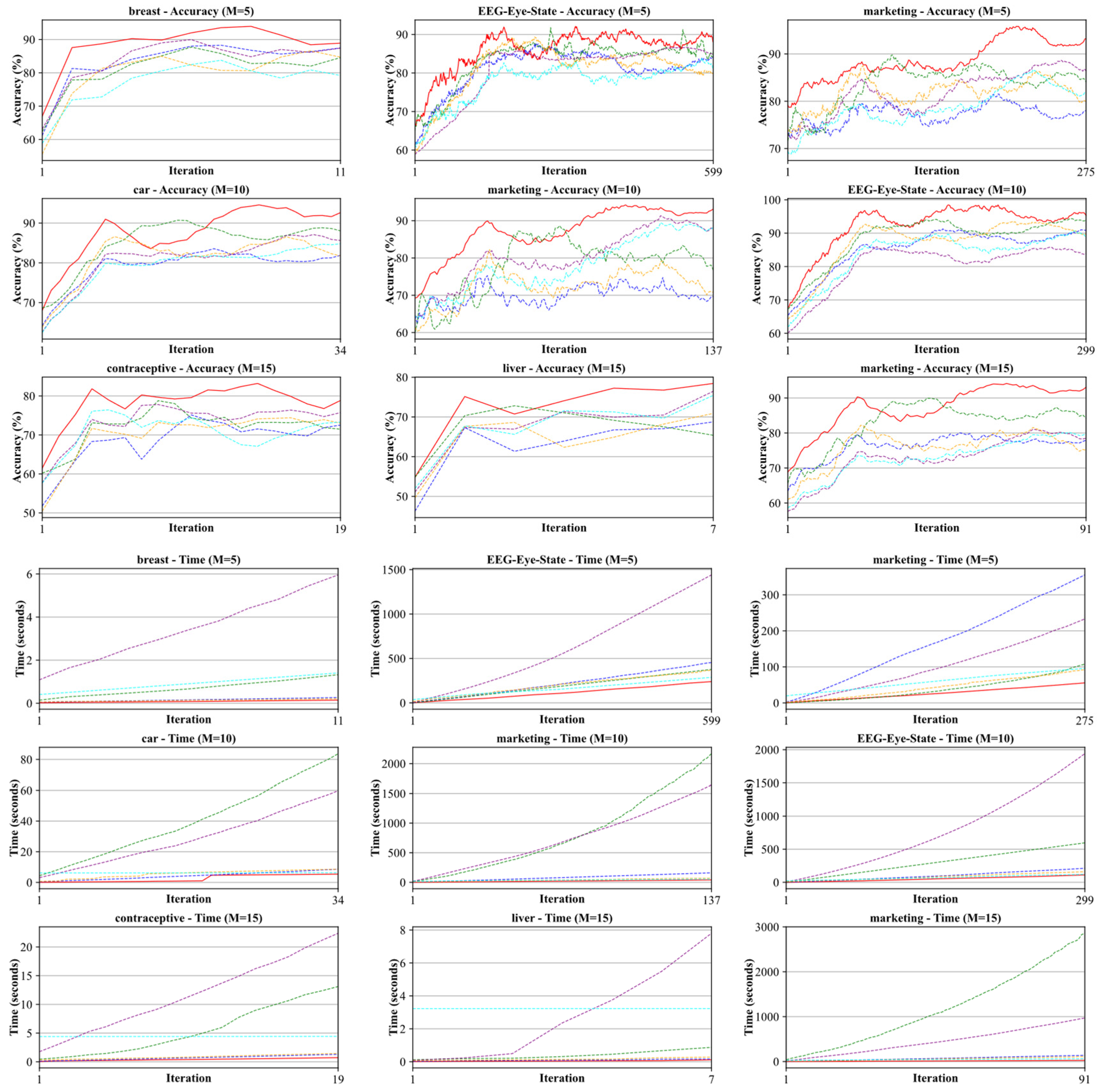
B-DIA-TSK processes multiple samples in batches and utilizes advanced mathematical methods, such as the Woodbury matrix identity and Cholesky decomposition, to optimize the inverse matrix computation process. This optimization significantly reduces the computational time and lowers the potential for error accumulation. This strategy not only improves the model’s computational efficiency when dealing with large-scale data sets but also enhances its stability and accuracy when processing high-dimensional data. Compared to traditional batch incremental learning algorithms, B-DIA-TSK was found to excel in handling large-scale data sets under resource-constrained computational environments, maintaining both efficient computational performance and high model accuracy and robustness. In particular, it demonstrated powerful adaptability and efficient resource utilization in complex data scenarios. From Figure 2, it can be further observed that significant concept drift emerged for the data sets EEG-Eye-Stage, marketing, liver and contraceptive. The classification accuracies of the comparative methods ILDA (chunk), MvIDA, OSELM (chunk), CICSHL-SVM and KB-IELM declined to different extents, while the proposed B-DIA-TSK maintained a significant advantage in terms of classification performance.

In general, O-DIA-TSK and B-DIA-TSK were found to strike an excellent balance between model simplification and high-performance efficiency. They successfully reduce unnecessary time complexity while maintaining the effectiveness and accuracy of the model. This balance ensures greater linguistic interpretability, making the model’s predictions more transparent and understandable. Furthermore, both algorithms exhibit outstanding generalization performance, maintaining stable high performance across different data sets and scenarios while significantly reducing computational costs and resource consumption. This enables O-DIA-TSK and B-DIA-TSK to demonstrate remarkable adaptability and robustness in various complex and dynamic data environments. Even in the event of concept drift, DIA-TSK still maintained a significant advantage in classification performance over the comparative methods. Whether in real-time data analysis, dynamic data processing or resource-limited computational settings, both algorithms effectively address various associated challenges and provide reliable solutions.

To further explore the performance advantages of O-DIA-TSK and B-DIA-TSK in incremental learning tasks, we conducted an additional analysis of the experimental results, presented in Figure 1 and Figure 2. In particular, we statistically calculated the average percentage improvement in time performance for O-DIA-TSK and B-DIA-TSK across the 16 different data sets. The research results are summarized in

Table 4. Computational efficiency and storage optimization comparison between the DIA-TSK framework and established online and incremental learning algorithms.

Method Type	Average Time Improvement (%)	Average Storage Performance Improvement (%)
O-DIA-TSK vs. FM3	32.13	28.64
O-DIA-TSK vs. ILDA (sequential)	30.91	13.40
O-DIA-TSK vs. LASVMG	32.41	82.28
O-DIA-TSK vs. OnlineSVM (Markov)	28.65	43.35
O-DIA-TSK vs. OSELM (sequential)	37.72	70.27
B-DIA-TSK vs. ILDA (chunk)	77.61	50.76
B-DIA-TSK vs. MvIDA	41.47	47.84
B-DIA-TSK vs. OSELM (chunk)	26.27	59.99
B-DIA-TSK vs. CICSHL-SVM	89.48	28.63
B-DIA-TSK vs. KB-IELM	78.27	36.2
B-DIA-TSK vs. O-DIA-TSK	73.21	56.38

, presenting the significant performance advantages exhibited by O-DIA-TSK and B-DIA-TSK in handling complex data environments. Ultimately, the findings further confirm the superior efficiency of O-DIA-TSK and B-DIA-TSK, fully demonstrating the improvements they bring to incremental learning tasks. It can also be observed, from Table 4, that B-DIA-TSK required less training time than O-DIA-TSK. This is because the fuzzy membership of the incremental training samples for the fuzzy rules can be calculated in parallel, as shown in Steps 4.1 and 4.3 in Algorithm 2.

4.5. Application to Real-World Data

In this section, in order to further validate the effectiveness of the O-DIA-TSK and B-DIA-TSK classifiers in handling incremental learning tasks, these methods were applied to the Bupa data set provided by KEEL. This data set contains 345 instances, including 145 instances with liver disease (labeled as 1) and 200 instances without liver disease (labeled as 2). Each instance is characterized by six features, which are representative of those associated with liver function in the medical field.

To compare the incremental learning performance of O-DIA-TSK and B-DIA-TSK, we randomly and exclusively selected 50% of the samples from the data set (i.e., 173 instances) as the initial training set, 30% (i.e., 104 instances) as the incremental training set and the remaining 20% (i.e., 68 instances) as the testing set. All methods learned the training samples in the same order. The experimental procedure involved multiple rounds of incremental learning in order to observe the model’s performance in a continuously updated data environment. The experimental results are shown in Figure 3 and Figure 4.

In this experiment, we applied the O-DIA-TSK and B-DIA-TSK incremental learning models to a real-world engineering data set and conducted a comparative analysis with various existing incremental learning classifiers. The experimental results revealed that these two models exhibit outstanding performance on this data set. First, O-DIA-TSK significantly enhanced the model’s real-time adaptability and classification performance through gradually adding individual samples and dynamically adjusting the prediction accuracy. Compared to traditional online learning methods, such as FM3 and OS-ELM (sequential), O-DIA-TSK not only achieved higher accuracy but also significantly reduced the time complexity. Particularly in scenarios where the data stream continuously increases, O-DIA-TSK demonstrates superior real-time processing capabilities, proving its applicability and efficiency on this data set.

Furthermore, B-DIA-TSK exhibited excellent computational efficiency in handling batch incremental learning tasks on this data set. Through utilization of the Woodbury matrix identity for matrix updates, B-DIA-TSK reduces computational resource consumption while significantly shortening the processing time. The experimental data indicated that B-DIA-TSK outperformed traditional batch incremental learning classifiers, such as OS-ELM (chunk) and ILDA (chunk), in terms of time efficiency when handling complex and dynamic data environments.

In conclusion, both O-DIA-TSK and B-DIA-TSK demonstrated exceptional classification performance on this specific data set. They not only outperformed the traditional incremental learning methods in terms of accuracy and computational efficiency but also further enhanced the model’s generalization ability and adaptability through the use of flexible and efficient model adjustment mechanisms. These results highlight the significant advantages and practical application value of the proposed models on the considered data set.

4.6. Significance Analysis

In this study, we aimed to assess the performance of incremental learning classifiers—including O-DIA-TSK and B-DIA-TSK—across multiple data sets through significance testing. The core purpose of the significance test was to determine whether there were statistically significant differences in the performance of these classifiers across different data sets. To achieve this goal, we employed the Friedman test for initial significance testing, and, upon detecting significant differences, we conducted post hoc tests to further analyze the specific sources of these differences.

To compare the performance of the two classifiers across different data sets, we first ranked their performance on each data set based on their specific evaluation metrics. Specifically, O-DIA-TSK and B-DIA-TSK were evaluated using the average accuracy as a metric. For each classifier on each data set, we calculated its ranking $R_v^u$, where $u$ denotes the classifier number, with $u\in \{1,\dots ,U\}$ and $U$ representing the total number of classifiers; $v$ denotes the data set number, with $v\in \{1,\dots ,V\}$, and $V$ is the total number of data sets; and $R_v^u$ indicates the ranking of classifier $u$ on data set $v$. Based on these ranking data, we used the following statistical formula for the Friedman test statistic $\Omega$ to assess the overall performance differences across all data sets:

$$\Omega ={\displaystyle \frac{12V}{U(U+1)}}\left[\sum _u^U {\underset{\_}{R}}_u^2-{\displaystyle \frac{U{\left(U+1\right)}^2}{4}}\right],\mathrm{}$$

(62)

where ${\underset{\_}{R}}_u$ is the average ranking of classifier $u$ across all data sets, calculated as

$${\underset{\_}{R}}_u=1/V\sum _{v=1}^V R_u^v\mathrm{}.$$

(63)

Once the value of $\Omega$ is obtained, the next step is to calculate the corresponding $p$-value in order to determine whether there are significant differences between the classifiers. When the number of classifiers $U>4$ and the number of data sets $V>15$, the distribution of the Friedman test statistic $\Omega$ approximates a chi-squared distribution with $U-1$ degrees of freedom. The calculation of the $p$-value was carried out as follows:

$$p=P\left({\chi }_{\alpha \left[U-1\right]}^2\ge \Omega \right).$$

(64)

The $p$-value is the result of the significance test, indicating whether the observed result is statistically significant. ${\chi }_{\alpha [U-1]}^2$ is the critical value of the chi-squared distribution with $U-1$ degrees of freedom, and $\alpha$ is typically set to 0.05. If the computed $p$-value is smaller than the pre-defined significance level $\alpha =0.05$, it indicates that there are significant differences in the performance of the classifiers across the data sets. In this case, we rejected the null hypothesis (i.e., assuming no significant difference between classifiers) and concluded that there is a statistically significant difference between the classifiers. When the Friedman test results showed significant differences, we performed further post hoc tests to identify and compare the specific differences between classifiers, including methods such as those of Hochberg, Holm and Hommel, which are used to conduct pairwise comparisons between classifiers in terms of their performance and adjust the $p$-values to address the multiple comparison problem, ensuring the reliability of the results.

The Friedman test results for the B-DIA-TSK and O-DIA-TSK classifiers and their average rankings are presented in

Table 5. Average rankings of the O-DIA-TSK and comparative methods (Friedman).

Method	Ranking
O-DIA-TSK	1
LASVMG	3.25
FM3	3.75
OSELM (sequential)	4
OnlineSVM (Markov)	4.5
ILDA (sequential)	4.5

and

Table 6. Average rankings of the B-DIA-TSK and comparative methods (Friedman).

Method	Ranking
B-DIA-TSK	1
CICSHL-SVM	2.8333
KB-IELM	3.1667
MvIDA	4.1667
OSELM (chunk)	4.6667
ILDA (chunk)	5.1667

.

The $p$-value obtained from the Friedman test was 0, indicating significant differences between the two classifiers compared to other baseline methods. From Table 5, we can observe that the O-DIA-TSK algorithm achieved the lowest average ranking of 1 in the Friedman test, suggesting that its overall performance was superior to that of the other methods. The LASVMG algorithm followed closely, with an average ranking of 3.25, while the FM3 and OSELM (sequential) algorithms ranked 3.75 and 4, respectively. The ILDA (sequential) and OnlineSVM (Markov) algorithms both had average rankings of 4.5, indicating relatively poorer performance. As shown in Table 6, the B-DIA-TSK method achieved an average ranking of 1, significantly outperforming the other methods and indicating its overall superior performance among the algorithms studied.

To further confirm the significant differences between classifiers, this study conducted a Holm–Hommel post hoc test on the Friedman test results and adjusted the multiple hypothesis tests using the Holm–Hommel method. The results of the post hoc tests are shown in

Table 7. Post hoc comparison table for O-DIA-TSK and comparative methods ($\alpha =0.05$, Friedman).

$\mathit{\delta }$	Method	$\mathit{z}=({\mathit{R}}_0-{\mathit{R}}_{\mathit{\delta }})/\mathit{S}\mathit{E}$	p	Holm–Hommel
5	ILDA (sequential)	2.835884	0.0046556	0.01
4	OnlineSVM (Markov)	2.646927	0.0081399	0.0125
3	OSELM (sequential)	2.344797	0.0187357	0.016667
2	FM3	2.079711	0.037525	0.025
1	LASVMG	1.701575	0.088973	0.05

and

Table 8. Post hoc comparison table for B-DIA-TSK and comparative methods ($\alpha =0.05$, Friedman).

$\mathit{\delta }$	Method	$\mathit{z}=({\mathit{R}}_0-{\mathit{R}}_{\mathit{\delta }})/\mathit{S}\mathit{E}$	p	Holm–Hommel
5	ILDA (chunk)	3.857584	0.000115	0.01
4	OSELM (chunk)	3.394674	0.000687	0.0125
3	MvIDA	2.931764	0.00337	0.016667
2	KB-IELM	2.005944	0.004486	0.025
1	CICSHL-SVM	1.697337	0.089633	0.05

, which further validate the significant accuracy differences for O-DIA-TSK and B-DIA-TSK.

According to the results presented in Table 7, the O-DIA-TSK method was significantly superior to the other comparative methods. Post hoc analysis of the Friedman test results revealed statistically significant differences between O-DIA-TSK and other algorithms. Specifically, the $z$-values for ILDA (sequential) and OnlineSVM (Markov) were both 2.645751, with unadjusted $p$-values of 0.008151, corresponding to Holm–Hommel critical values of 0.01 and 0.0125. As the unadjusted $p$-values were smaller than the corresponding Holm–Hommel critical values, the performance differences between these methods and O-DIA-TSK were statistically significant. Similarly, the $z$-value for OSELM (sequential) was 2.267787, with a $p$-value of 0.013342, which is also smaller than its Holm–Hommel critical value of 0.016667, confirming a significant difference. For FM3, the $z$-value was 2.078805, with an unadjusted $p$-value of 0.037635, slightly below the Holm–Hommel critical value of 0.045, thus still indicating a statistically significant difference. These results demonstrate that the O-DIA-TSK method outperformed the ILDA (sequential), OnlineSVM (Markov), OSELM (sequential) and FM3 methods. Although the p-values for OSELM (sequential), FM3 and LASVMG in Table 7 and Table 8 were bigger than the corresponding Holm–Hommel values, the corresponding very low p-values still indicate the competitive nature of O-DIA-TSK. In summary, the O-DIA-TSK method demonstrated superior overall performance compared to most other comparison algorithms, which was rigorously validated in a statistical manner.

As detailed in Table 8, the B-DIA-TSK method also significantly outperformed the other comparative methods. Post hoc analysis of the Friedman test results revealed substantial differences between B-DIA-TSK and the other algorithms. Specifically, the $z$-value for ILDA (chunk) was 3.857584, with a $p$-value of 0.000115 and adjusted Holm–Hommel significance level of 0.01. As the $p$-value is smaller than the significance level, the difference is statistically significant. Similarly, the $p$-values for OSELM (chunk), MvIDA and KB-IELM were 0.000687, 0.00337 and 0.004486, respectively, all smaller than their corresponding Holm–Hommel critical values, indicating statistically significant differences between these methods and B-DIA-TSK. Although the p-value for CICSHL-SVM in Table 8 exceeded the corresponding Holm–Hommel threshold, their notably low magnitude demonstrates the competitive performance of B-DIA-TSK. These results indicate that B-DIA-TSK not only shows significant improvements in performance over most compared methods but also delivered the best overall performance.

For a more comprehensive analysis, we also computed the adjusted $p$-values for the post hoc tests, as shown in

Table 9. Adjusted p-values for O-DIA-TSK and comparative methods (Friedman).

$\mathit{\delta }$	Method	Unadjusted p	p (Holm)	p (Hommel)
1	ILDA (sequential)	0.0046556	0.023278	0.0186224
2	OnlineSVM (Markov)	0.0081399	0.0325596	0.0244197
3	OSELM (sequential)	0.0187357	0.0374714	0.0321222
4	FM3	0.037625	0.037525	0.037525
5	LASVMG	0.088973	0.088973	0.088973

and

Table 10. Adjusted p-values for B-DIA-TSK and comparative methods (Friedman).

$\mathit{\delta }$	Method	Unadjusted p	p (Holm)	p (Hommel)
1	ILDA (chunk)	0.000115	0.000573	0.000573
2	OSELM (chunk)	0.000687	0.002748	0.002748
3	MvIDA	0.00337	0.010111	0.010111
4	KB-IELM	0.004486	0.008972	0.008963
5	CICSHL-SVM	0.089633	0.089725	0.089633

. The adjusted $p$-values were obtained by applying the post hoc methods from the Friedman test.

As can be seen from Table 9, the adjusted $p$-values further confirmed the exceptional performance of O-DIA-TSK. Specifically, the unadjusted $p$-values for ILDA (sequential) and OnlineSVM (Markov) were both 0.008151, and, after adjustment using the Holm and Hommel methods, these values became 0.040755 and 0.032604—both lower than the significance level. This confirms that even after multiple comparison and correction, the performance differences between O-DIA-TSK and these two methods are still statistically significant. Similarly, the adjusted $p$-values for OSELM (sequential) and FM3 were also close to or below the significance level, further supporting the superiority of O-DIA-TSK. Although the adjusted $p$-value for LASVMG was 0.088973—and, thus, slightly higher than the significance level—O-DIA-TSK clearly presented better overall performance. Combined with the results of the Friedman test and post hoc analysis, it can be conclusively stated that O-DIA-TSK outperformed the algorithms studied, and its performance advantage was rigorously statistically validated.

Based on the adjusted $p$-values shown in Table 10, the superior performance of B-DIA-TSK was also further validated. Specifically, the unadjusted $p$-value for ILDA (chunk) was 0.000115, while after adjustment, the $p$-values were 0.000573, far below the significance level of $\alpha =0.05$. This indicates that even after correction for multiple comparisons, the performance difference between B-DIA-TSK and ILDA (chunk) remains highly statistically significant. Similarly, the adjusted $p$-values for OSELM (chunk), MvIDA and KB-IELM were 0.002748, 0.010111 and 0.008972, respectively, all significantly smaller than 0.05, further supporting the superior performance of B-DIA-TSK. Notably, the (Hommel) adjusted $p$-value for CICSHL-SVM was 0.089633, slightly above the significance level, meaning that the performance difference between CICSHL-SVM and B-DIA-TSK is not statistically significant; however, B-DIA-TSK still holds the highest average ranking, confirming its superior performance overall. These results conclusively demonstrate that B-DIA-TSK delivers the best performance among the algorithms studied, and its performance advantage was rigorously statistically validated.

In conclusion, the DIA-TSK classifiers outperformed the other online and batch incremental learning classifiers and exhibited significant advantages—particularly in terms of accuracy—thus indicating their robustness and reliability in dynamic data environments.

5. Conclusions

The DIA-TSK approach was proposed in this study, which is based on the zero-order TSK fuzzy classifier for online and incremental learning. In contrast to the static approach used in existing online and incremental learning methods, the parameters of DIA-TSK can be adjusted in real time, effectively maintaining a global optimum during the incremental training process. Extensive experimental evaluations involving incremental training processes demonstrated the DIA-TSK methods to be superior, in terms of classification performance, with respect to comparative methods. In particular, when concept drift occurred, DIA-TSK obtained 10% higher classification accuracy than the comparative methods on average, and, in terms of time efficiency, the training process of DIA-TSK methods took 30% less time than comparative methods.

Future research can focus on the following areas: (1) improving the DIA-TSK to better deal with dynamic data characterized by drastic changes in distribution, number of features and/or number of classes; (2) expanding DIA-TSK with different fuzzy systems (e.g., high-order TSK fuzzy systems and Mamdani fuzzy systems) in order to derive novel online and incremental fuzzy classifiers with different characteristics; and (3) further improving DIA-TSK to resolve the classification problem of class-imbalanced data in practical applications. (4) Due to the similarity between the TSK fuzzy classifiers and artificial neural networks, there is substantial potential to expand the methodology of DIA-TSK to artificial neural networks in order to improve its real-time capabilities.

References

1. Zadeh, L.A. On fuzzy algorithms. In Fuzzy Sets, Fuzzy Logic, and Fuzzy Systems: Selected Papers; World Scientific Publishing Co., Pte. Ltd.: Singapore, 1996; pp. 127–147. [Google Scholar]
2. Ying, H.A.O.; Chen, G. Necessary conditions for some typical fuzzy systems as universal approximators. Automatica 1997, 33, 1333–1338. [Google Scholar] [CrossRef]
3. Wong, S.Y.; Yap, K.S.; Yap, H.J.; Tan, S.C.; Chang, S.W. On equivalence of FIS and ELM for interpretable rule-based knowledge representation. IEEE Trans. Neural Netw. Learn. Syst. 2014, 26, 1417–1430. [Google Scholar] [PubMed]
4. Yang, C.F.; Chen, C.L.; Wang, Y.S. Interval type-2 TSK fuzzy neural model for illuminant estimation. In Proceedings of the 2016 12th IEEE International Conference on Control and Automation (ICCA), Kathmandu, Nepal, 1–3 June 2016; pp. 517–522. [Google Scholar]
5. Karaboga, D.; Kaya, E. An adaptive and hybrid artificial bee colony algorithm (aABC) for ANFIS training. Appl. Soft Comput. 2016, 49, 423–436. [Google Scholar]
6. Pramod, C.P.; Pillai, G.N. K-Means clustering based Extreme Learning ANFIS with improved interpretability for regression problems. Knowl.-Based Syst. 2021, 215, 106750. [Google Scholar]
7. Ishibuchi, H.; Nozaki, K.; Yamamoto, N.; Tanaka, H. Selecting fuzzy if-then rules for classification problems using genetic algorithms. IEEE Trans. Fuzzy Syst. 1995, 3, 260–270. [Google Scholar]
8. Lin, C.T.; Pal, N.R.; Wu, S.L.; Liu, Y.T.; Lin, Y.Y. An interval type-2 neural fuzzy system for online system identification and feature elimination. IEEE Trans. Neural Netw. Learn. Syst. 2014, 26, 1442–1455. [Google Scholar]
9. Zhou, S.M.; Gan, J.Q. Constructing L2-SVM-based fuzzy classifiers in high-dimensional space with automatic model selection and fuzzy rule ranking. IEEE Trans. Fuzzy Syst. 2007, 15, 398–409. [Google Scholar]
10. Lu, J.; Zuo, H.; Zhang, G. Fuzzy multiple-source transfer learning. IEEE Trans. Fuzzy Syst. 2019, 28, 3418–3431. [Google Scholar]
11. Jhang, J.Y.; Lin, C.J.; Kuo, S.W. Convolutional Takagi-Sugeno-Kang-type Fuzzy Neural Network for Bearing Fault Diagnosis. Sens. Mater. 2023, 35, 2355. [Google Scholar] [CrossRef]
12. Hu, K.; Bi, Z.; He, Q.; Peng, Z. A feature extension and reconstruction method with incremental learning capabilities under limited samples for intelligent diagnosis. Adv. Eng. Inform. 2024, 62, 102796. [Google Scholar] [CrossRef]
13. Hua, S.; Wang, C.; Lam, H.K.; Wen, S. An incremental learning method with hybrid data over/down-sampling for sEMG-based gesture classification. Biomed. Signal Process. Control 2023, 83, 104613. [Google Scholar] [CrossRef]
14. Feng, L.; Zhao, C.; Chen, C.L.P.; Li, Y.; Zhou, M.; Qiao, H.; Fu, C. BNGBS: An efficient network boosting system with triple incremental learning capabilities for more nodes, samples, and classes. Neurocomputing 2020, 412, 486–501. [Google Scholar] [CrossRef]
15. Zheng, T.; Cheng, L.; Gong, S.; Huang, X. Model incremental learning of flight dynamics enhanced by sample management. Aerosp. Sci. Technol. 2025, 160, 110049. [Google Scholar] [CrossRef]
16. Zhang, Y.; Wang, G.; Zhou, T.; Huang, X.; Lam, S.; Sheng, J.; Ding, W. Takagi-Sugeno-Kang fuzzy system fusion: A survey at hierarchical, wide and stacked levels. Inf. Fusion 2024, 101, 101977. [Google Scholar]
17. Wu, X.; Jiang, B.; Wang, X.; Ban, T.; Chen, H. Feature Selection in the Data Stream Based on Incremental Markov Boundary Learning. IEEE Trans. Neural Netw. Learn. Syst. 2023, 34, 6740–6754. [Google Scholar]
18. Ren, M.; Liu, F.; Wang, H.; Zhang, Z. Addressing Concept Drift in Active Learning for TSK Fuzzy Systems. IEEE Trans. Fuzzy Syst. 2023, 31, 608–621. [Google Scholar]
19. Li, Y.; Zhou, E.; Vong, C.M.; Wang, S. Stacked Ensemble of Extremely Interpretable Takagi–Sugeno–Kang Fuzzy Classifiers for High-Dimensional Data. IEEE Trans. Syst. Man Cybern. Syst. 2025, 55, 2414–2425. [Google Scholar]
20. Hernández, H.; Díaz-Viera, M.A.; Alberdi, E.; Goti, A. Comparison of Trivariate Copula-Based Conditional Quantile Regression Versus Machine Learning Methods for Estimating Copper Recovery. Mathematics 2025, 13, 576. [Google Scholar] [CrossRef]
21. Ji, R.; Chen, Z.; Li, Y.; Wu, P. Resource-Efficient Active Learning Framework for Large-Scale TSK Fuzzy Systems. IEEE Trans. Syst. Man Cybern. Syst. 2024, 54, 245–257. [Google Scholar]
22. Guo, Y.; Zheng, Z.; Pu, J.; Jiao, B.; Gong, D.; Yang, S. Robust online active learning with cluster-based local drift detection for unbalanced imperfect data. Appl. Soft Comput. 2024, 165, 112051. [Google Scholar] [CrossRef]
23. Xue, L.; Wang, J.; Qin, Y.; Zhang, Y.; Yang, Q.; Li, Z. Two-timescale online coordinated schedule of active distribution network considering dynamic network reconfiguration via bi-level safe deep reinforcement learning. Electr. Power Syst. Res. 2024, 234, 110549. [Google Scholar] [CrossRef]
24. Guo, Y.; Pu, J.; Jiao, B.; Peng, Y.; Wang, D.; Yang, S. Online semi-supervised active learning ensemble classification for evolving imbalanced data streams. Appl. Soft Comput. 2024, 155, 111452. [Google Scholar] [CrossRef]
25. Fan, W.; Yang, W.; Chen, T.; Guo, Y.; Wang, Y. AOCBLS: A novel active and online learning system for ECG arrhythmia classification with less labeled samples. Knowl.-Based Syst. 2024, 304, 112553. [Google Scholar] [CrossRef]
26. Malialis, K.; Panayiotou, C.G.; Polycarpou, M.M. Nonstationary data stream classification with online active learning and siamese neural networks. Neurocomputing 2022, 512, 235–252. [Google Scholar]
27. Zhang, J.; Li, Y.; Liu, B.; Chen, H.; Zhou, J.; Yu, H.; Qin, B. A Broad TSK Fuzzy Classifier with a Simplified Set of Fuzzy Rules for Class-Imbalanced Learning. Mathematics 2023, 11, 4284. [Google Scholar] [CrossRef]
28. Castorena, G.A.H.; Méndez, G.M.; López-Juárez, I.; García, M.A.A.; Martinez-Peon, D.C.; Montes-Dorantes, P.N. Parameter prediction with Novel enhanced Wagner Hagras interval Type-3 Takagi–Sugeno–Kang Fuzzy system with type-1 non-singleton inputs. Mathematics 2024, 12, 1976. [Google Scholar] [CrossRef]
29. Yang, Q.; Gu, Y.; Wu, D. Survey of incremental learning. In Proceedings of the 2019 Chinese Control and Decision Conference (CCDC), Nanchang, China, 3–5 June 2019. [Google Scholar]
30. Qin, B.; Nojima, Y.; Ishibuchi, H.; Wang, S. Realizing deep high-order TSK fuzzy classifier by ensembling interpretable zero-order TSK fuzzy subclassifiers. IEEE Trans. Fuzzy Syst. 2021, 29, 3441–3455. [Google Scholar] [CrossRef]
31. Wang, S.; Jiang, Y.; Chung, F.L.; Qian, P. Feedforward kernel neural networks, generalized least learning machine, and its deep learning with application to image classification. Appl. Soft Comput. 2015, 37, 125–141. [Google Scholar]
32. Qin, B.; Chung, F.; Wang, S. KAT: A knowledge adversarial training method for zero-order Takagi–Sugeno–Kang fuzzy classifiers. IEEE Trans. Cybern. 2022, 52, 6857–6871. [Google Scholar]
33. Cheng, W.Y.; Juang, C.F. A fuzzy model with online incremental SVM and margin-selective gradient descent learning for classification problems. IEEE Trans. Fuzzy Syst. 2013, 22, 324–337. [Google Scholar]
34. Ertekin, S.; Bottou, L.; Giles, C.L. Nonconvex online support vector machines. IEEE Trans. Pattern Anal. Mach. Intell. 2010, 33, 368–381. [Google Scholar] [CrossRef] [PubMed]
35. Xu, J.; Tang, Y.Y.; Zou, B.; Xu, Z.; Li, L.; Lu, Y. The generalization ability of online SVM classification based on Markov sampling. IEEE Trans. Neural Netw. Learn. Syst. 2014, 26, 628–639. [Google Scholar] [PubMed]
36. Liang, N.Y.; Huang, G.B.; Saratchandran, P.; Sundararajan, N. A fast and accurate online sequential learning algorithm for feedforward networks. IEEE Trans. Neural Netw. 2006, 17, 1411–1423. [Google Scholar] [PubMed]
37. Pang, S.; Ozawa, S.; Kasabov, N. Incremental linear discriminant analysis for classification of data streams. IEEE Trans. Syst. Man Cybern. Part B (Cybern.) 2005, 35, 905–914. [Google Scholar]
38. Gu, B.; Quan, X.; Gu, Y.; Sheng, V.S.; Zheng, G. Chunk incremental learning for cost-sensitive hinge loss support vector machine. Pattern Recognit. 2018, 83, 196–208. [Google Scholar]
39. Guo, L.; Hao, J.H.; Liu, M. An incremental extreme learning machine for online sequential learning problems. Neurocomputing 2014, 128, 50–58. [Google Scholar] [CrossRef]
40. Shivagunde, S.S.; Nadapana, A.; Saradhi, V.V. Multi-view incremental discriminant analysis. Inf. Fusion 2021, 68, 149–160. [Google Scholar]
Figure 1. Comparison of accuracy and time performance of O-DIA-TSK and online learning classifiers across multiple data sets. Red line denotes the experimental result of O-DIA-TSK; blue line denotes the experimental result of FM3; green line denotes the experimental result of LASVMG; brown line denotes the experimental result of OnlineSVM (Markov); purple line denotes the experimental result of OSELM (sequential); cyan line denotes the experimental result of ILDA (sequential).
Mathematics 13 01054 g001aMathematics 13 01054 g001b
Figure 2. Comparison of accuracy and time performance of B-DIA-TSK and batch incremental learning classifiers across multiple data sets. Red line denotes the experimental result of B-DIA-TSK; blue line denotes the experimental result of ILDA (chunk); purple line denotes the experimental result of MvIDA; cyan line denotes the experimental result of OSELM (chunk); green line denotes the experimental result of CICSHL-SVM; brown line denotes the experimental result of KB-IELM.
Mathematics 13 01054 g002
Figure 3. Performance of the O-DIA-TSK method on the Bupa data set. Red line denotes the experimental result of O-DIA-TSK; blue line denotes the experimental result of FM3; green line denotes the experimental result of LASVG; brown line denotes the experimental result of OnlineSVM (Markov); purple line denotes the experimental result of OSELM (sequential); cyan line denotes the experimental result of ILDA (sequential).
Mathematics 13 01054 g003
Figure 4. Performance of the B-DIA-TSK method on Bupa data set. Red line denotes the experimental result of B-DIA-TSK; blue line denotes the experimental result of ILDA (chunk); purple line denotes the experimental result of MvIDA; cyan line denotes the experimental result of OSELM (chunk); green line denotes the experimental result of CICSHL-SVM; brown line denotes the experimental result of KB-IELM.
Mathematics 13 01054 g004