A Solution Method for Partial Differential Equations by Fusing Fourier Operators and U-Net

Abstract

In scientific and engineering calculation, the effective solution of partial differential equations (PDEs) has great significance. This paper presents an innovative method based on the combination of a U-Net neural network with Fourier neural operators, aiming to improve the accuracy and efficiency of solving partial differential equations. U-Net neural networks with a unique encoding–decoder structure and hopping connections can efficiently extract and integrate spatial-domain features and accurately describe the spatial structure of PDEs. The Fourier neural operator combines the advantages of neural networks and Fourier transform to learn the mapping relationship of high-dimensional data by training the linear transformation parameters in the detailed frequency domain of the data. Fourier transform is used to explore and process the frequency-domain features and capture the frequency characteristics of the solution of partial differential equations. By combining the two, this method not only retains spatial details but also makes full use of frequency-domain information, which significantly reduces the dependence of the model on large-scale data and improves the generalization ability of the model. The experimental results show that compared with the traditional method, this method performs well in various complex partial differential equation (PDE) solving tasks and achieves high accuracy.

1. Introduction

In fluid mechanics, geophysics, biology, and many other fields, the partial differential equation (PDE) model serves as a crucial tool for characterizing various phenomena. Related problems encompass physical model building, the solution of partial differential equations, and parameter inversion. The process of solving a partial differential equation involves obtaining a spatially accurate solution or a numerical solution under the known partial differential equation and other constraints [1,2,3,4].

Traditional numerical solution methods for partial differential equations rely on a discrete scheme based finite difference systems, commonly referred to as the computational fluid dynamics (CFD) method. Examples include the Runge–Kutta method, the prediction correction method, the finite element method [5], the finite difference method [6], and the finite volume method [7], among others. In contrast to traditional solving methods, neural networks exhibit distinct advantages in solving differential equations. Neural networks possess a powerful data fitting capacity, and even a small-scale neural network can handle simple partial differential equations [8]. Employing the neural network approach to solve differential equations effectively addresses issues such as poor adaptability and conditional limitations of grid sections. Compared with traditional numerical methods, the neural network method requires fewer sampling points to achieve higher accuracy. Moreover, once a neural network model is trained, it can be directly utilized to calculate the numerical results at any point within the obtained domain. Starting in the 1990s, scholars initiated research on the mathematical foundations and methods of using neural networks to solve differential equations. In 1990, Hornik et al. [9] demonstrated that under certain conditions, a multilayer neural network can approximate any function and its derivative, even when the function only has a generalized derivative. This finding laid the groundwork for neural network-based solutions to partial differential equations. In 1998, Lagaris and Likas [10] put forward a method for solving the first boundary value problem using an artificial neural network (ANN). In 2011, Kumar and Yadav [11] investigated multilayer neural network (MLP) and radial basis function neural network (RBF) models for solving differential equations and compared and summarized the applications of MLP and RBF in this regard. In 2018, Winovich et al. [12] proposed a quantitative uncertainty convolutional neural network (ConvPDE-UQ) for the problem of heterogeneous elliptic partial differential equations on different domains. Also in 2018, Long and Dong et al. [13,14] introduced a novel feed-forward neural network (PDE-Net). Its core concept is to approximate the differential operator with a convolution kernel, construct a network to approximate the nonlinear partial differential equation system, and achieve long-term prediction of its solution. A convolutional network is essentially an input-to-output mapping capable of learning numerous mapping relationships between input and output without the need for any precise mathematical expressions between them. However, due to the increase in dimensions, the solution accuracy of the convolutional neural network model [15] is slightly diminished. Most of the above-mentioned neural network-based methods for solving partial differential equations are focused on the initial boundary value problem. The network takes space coordinates or time variables as inputs and outputs the solution values in space. When constructing solutions by integrating partial differential equations with neural networks, the optimization objectives typically consist of two parts: the errors at the initial solution and boundary value sampling points and the errors at the sampling points within the domain subject to the differential equation constraints.

In addition, when we need to rapidly obtain accurate solutions for a set of partial differential equations, one approach we can adopt is the neuronal operator method. This method can be learned based on the mapping from the source-term function to the solution function of the partial differential equation set [16].

Fourier transform holds a significant position in deep learning models. It aids in the proof of the universal approximation theorem [17] and can also accelerate the training of convolutional neural networks [18]. Keivan Alizadeh Vahid et al. [19] proposed the extension of the butterfly operation in traditional fast Fourier transform and its application to the design of convolutional neural network architectures. They demonstrated that the computational complexity of the alternative network layer through butterfly transformation was reduced from N to $NlogN$. Experiments also confirmed that the proposed scheme effectively enhanced the model’s accuracy. Integrating Fourier transform into the neural network model can effectively decrease the model’s computational complexity. Moreover, the physical trends in the data can be effectively captured through Fourier transform, which offers great advantages for solving partial differential equations. Li [20] proposed the neural operator method, which can be evaluated at any point in time and in any space. Additionally, a general approximation theorem for neural operators was summarized and proven. Li [21] put forward the Fourier neural operator, where the integral operator operates directly in Fourier space through parameterization. Evidently, the neural operator approach is a fully data-driven method, necessitating a large number of high-quality datasets. However, in the analysis of complex physical, biological, or engineering systems, the cost of data acquisition is often prohibitively high. As a result, we inevitably encounter the challenge of drawing long-term conclusions with partial information, making these methods inefficient. Kushnure et al. [22] proposed an architecture named MS U-Net for multi-scale feature representation and recalibration. This architecture uses the Res2Net module to retain the contextual information of segmented objects, and it squeezes and motivates the network to recalibrate multi-scale feature channels, thereby enhancing the network’s ability to describe high-level features. In the literature [23], for the same data preprocessing process, the feature representations of each modality learned by the network are fused at later stages. In the last layer of convolution, a larger-scale feature map is connected to achieve the communication of contextual information between feature maps of different sizes.

This integration of multi-scale feature representation and recalibration mechanisms allows the network to better capture both local and global information, which is crucial for solving complex partial differential equations. By leveraging these advanced techniques, the model can achieve higher accuracy and efficiency in solving PDEs, even in scenarios where data are limited or incomplete.

In many applications in the fields of science and engineering, solving partial differential equations (PDEs) is a crucial task. The method of combining Fourier transform and neural operator recalibration provides a powerful framework for this task.

As one of the key technologies, Fourier transform can extract the information features in the frequency domain and accurately capture the key information of the equations. Meanwhile, convolutional neural networks can be used to extract the high-level internal features of the system. By adopting a connection-based mechanism to reduce the number of network layers, the relevant models can effectively solve PDEs from the global and internal characteristics of the system.

Take U-Net as an example. It extracts image features in the form of convolution, and its essence is to capture the changes in the image by calculating the derivatives of image pixels. In contrast, the Fourier neural operator calculates derivatives in the form of filter operators and achieves fast calculation with the help of convolution functions. By transforming the problem into the frequency domain, the Fourier operator can effectively capture the global features of the signal; reduce the impact of high-frequency noise; and, thus, improve the stability and accuracy of the solution [24].

Compared with many existing hybrid modeling methods, such as the combination of deep learning and traditional numerical methods proposed by M, F and J [25], they mainly rely on local modeling in the spatial domain and often ignore the globality of the frequency-domain features. Although this local modeling method is effective in some cases, when dealing with PDEs with complex boundary conditions and multi-scale features, it often encounters the dilemmas of low computational efficiency and insufficient accuracy.

The innovation of this study lies in combination of the powerful feature extraction ability of U-Net with the frequency-domain analysis ability of Fourier transform to construct a unified framework. Specifically, first, U-Net is used for local feature modeling in the spatial domain, which enhances the generalization ability of the network in dealing with nonlinear and high-dimensional problems. Subsequently, Fourier transform is used to convert the PDE into a frequency-domain representation to capture its global features and periodic information. This fusion strategy not only improves the solution efficiency but also significantly enhances the adaptability of the model in the face of complex physical phenomena.

Based on the above concepts, this study further proposes a U-Net neural network model based on the Fourier neural operator. This model uses multiple low-order constrained convolutional kernels to approximate high-order differential operators, thereby more accurately describing the properties of differential equations. In the model design, the feed-forward neural operator, as the core component, contains adjustable parameters that can be continuously optimized through training. This design not only improves the solution accuracy of the model but also provides support for long-term effective and stable numerical solutions.

2. Preliminaries

2.1. Parametric Partial Differential Equations

Let G be the nonlinear operator; general parametric PDEs can be expressed as $G(u,s)=0$, where u is the input function and s is the solution to an unknown partial differential equation (as well as a function).

Our PDE solution operator is $G(u)=s$.

We can express the general solution of our PDE as $G(u)(y)=s(y)$.

A common instantiation is the approximation of the second-order elliptic PDE:

$$\begin{array}{cccc}\hfill -\nabla ·(a(x)\nabla u(x))& =f(x),\hfill & \hfill & x\in D\hfill \end{array}$$

(1)

$$\begin{array}{cccc}\hfill u(x)& =0,\hfill & \hfill & x\in \partial D\hfill \end{array}$$

(2)

where u is our target solution object; $f(x)$ is the right end term, which is regarded as a forcing term in many physical equations; $a(x)$ is the $a\in \mathcal{A}$ parameter, where $\mathcal{A}$ is the parameter space. In operator form, we express it as follows:

$$\begin{array}{c}\hfill \left(L_{\alpha }u\right)(x)=f(x),x\in D\end{array}$$

(3)

$$\begin{array}{c}\hfill u(x)=0,x\in \partial D\end{array}$$

(4)

where ${\mathcal{L}}_a·=-div(a\nabla ·)$, where subscript a represents operator $\mathcal{L}$ for parameter a.

Under rather general conditions of ${\mathcal{L}}_a$, we can define the Green function ($G:D\times D\to \mathbb{R}$) as the unique solution to the following problem:

$${\mathcal{L}}_{a}G(·,x)={\delta }_x$$

(5)

To be concrete, we consider infinite-dimensional spaces, which are Banach spaces of real-valued functions defined on a bounded open set in ${\mathbb{R}}^d$. We then consider mappings (${\mathcal{F}}^{†}$) that take input functions to a PDE and map them to solutions of the PDE, with both input and solutions being real-valued functions on ${\mathbb{R}}^d$.

2.2. PDE Setting

Let $\mathcal{A}$ and U be separable Banach spaces and ${\mathcal{F}}^{†}:\mathcal{A}\to U$ be a (typically) nonlinear map.

Considering some bounded, open domain ($D\in \mathbb{R}$) and a fixed source function (f), for a given function (a), the equation has a unique weak solution (u), so we can define the solution operator (${\mathcal{F}}^{†}$) as the map ($a\to u$) of the function to second the function.

Our goal is to learn an operator ($\mathcal{F}$) to approximate ${\mathcal{F}}^{†}$ by using a limited set of observed input–output pairs (${\{a_j,u_j\}}_{j=1}^N$, where $a_j$ and $u_j$ are each a function on D).

We aim to build an approximation of ${\mathcal{F}}^{†}$ by constructing a parametric map, i.e.,

$$\begin{array}{c}\hfill \mathcal{F}:\mathcal{A}\times \theta \to U,\end{array}$$

(6)

for some finite-dimensional parameter space ($\theta$), then choosing ${\theta }^{†}\in \Theta$ so that $\mathcal{F}(·,{\theta }^{†})\approx {\mathcal{F}}^{†}$.

Therefore, our optimization goal is the minimization of the loss function, i.e.,

$$\underset{\theta \in R^p}{min}{E}_{a\sim u}\left|\right|{\mathcal{F}}^{†}(a)-{\mathcal{F}}_{\theta }{(a)\left|\right|}_u^2\approx \underset{\theta \in R^p}{min}{\displaystyle \frac{1}{N}}\sum _{i=1}^N\left|\right|u^{(i)}-{\mathcal{F}}_{\theta }(a^{(i)}){\left|\right|}_u^2,$$

(7)

which directly parallels the classical finite-dimensional setting.

3. Algorithm

3.1. Setting of Input Signal and Function Space

The input signal ($u(x)$) serves as the key factor for a model to gather characteristic information, and its quality sets the upper limit of the model’s achievable accuracy. In this paper, we primarily consider two function spaces:

The Orthogonal (Chebyshev) Polynomial Component of the Gaussian Random Field (GRF) and the Gaussian Random Field (GRF).

Typically, we employ a zero-mean Gaussian random field, expressed as follows:

$$\begin{array}{c}\hfill u\sim \mathcal{G}(0,k_l(x_1,x_2))\end{array}$$

(8)

where the covariance function is the Gaussian kernel given by

$$\begin{array}{c}\hfill k_l(x_1,x_2)=exp(-||x_1-x_2{\left|\right|}^2/2l^2)\end{array}$$

(9)

The length scale (l) is of great significance, as it determines the smoothness of the sampling function. When the value of l is large, the resulting u function is smoother, which is of great importance in studying phenomena at different scales.

After selecting the function space, sampling needs to be carried out from this space. The specific approach is to scatter points within the specified region to obtain sample points. Subsequently, $(u,x,y)$ is integrated, and the resulting value is used as the input data of the model. By constructing the model in this way, an approximate solution (y) is obtained. To comprehensively evaluate the performance of the model, multiple different test sets (u) are generated by randomly selecting data so as to examine the performance of the model under different data distributions.

Gaussian random field with the radial-basis function kernel:

Suppose there is a stochastic process ($X(t)$) that follows a specific Gaussian random-field distribution, that is, $X(t)\sim \mathcal{G}(0,exp(-{\displaystyle \frac{{|x-y|}^2}{l^2}}))$.

Then, $X(t)$ can be represented by the following integral form:

$$\begin{array}{cc}\hfill X(t)& =\sqrt{2}{(\pi )}^{{\displaystyle \frac{1}{4}}}{\int }_{{\mathbb{R}}^{+}}{(l)}^{{\displaystyle \frac{1}{2}}}cos(\omega t)exp(-{\displaystyle \frac{l^2{\omega }^2}{8}})dW(\omega )\hfill \\ & -\sqrt{2}{(\pi )}^{{\displaystyle \frac{1}{4}}}{\int }_{{\mathbb{R}}^{+}}{(l)}^{{\displaystyle \frac{1}{2}}}sin(\omega t)exp(-{\displaystyle \frac{l^2{\omega }^2}{8}})dB(\omega ),\hfill \end{array}$$

(10)

In the above expression, W and B are independent standard Brownian motions that introduce randomness to $X(t)$. To further simplify the expression, variable substitution is carried out, applying the change of variable corresponding to $\lambda =l\omega$. After the transformation, $X(t)$ can be rewritten as follows:

$$\begin{array}{c}\hfill X(t)=\sqrt{2}{(\pi )}^{{\displaystyle \frac{1}{4}}}{\int }_{{\mathbb{R}}^{+}}cos({\displaystyle \frac{\lambda }{l}}t)exp(-{\displaystyle \frac{{\lambda }^2}{8}})dW(\lambda )-\sqrt{2}{(\pi )}^{{\displaystyle \frac{1}{4}}}{\int }_{{\mathbb{R}}^{+}}sin({\displaystyle \frac{\lambda }{l}}t)exp(-{\displaystyle \frac{{\lambda }^2}{8}})dB(\lambda ).\end{array}$$

(11)

The, linear interpolation (${\Pi }_1$) is applied on the interval of $[t_i,t_{i+1}]$

$$\begin{array}{cc}\hfill \mathbb{E}\left[{(X(t)-{\Pi }_{1}X(t))}^2\right]& =2{(\pi )}^{{\displaystyle \frac{1}{2}}}{\int }_{{\mathbb{R}}^{+}}{((I-{\Pi }_1)cos({\displaystyle \frac{\lambda }{l}}t))}^{2}exp(-{\displaystyle \frac{{\lambda }^2}{4}})d\lambda \hfill \\ & +2{(\pi )}^{{\displaystyle \frac{1}{2}}}{\int }_{{\mathbb{R}}^{+}}{((I-{\Pi }_1)sin({\displaystyle \frac{\lambda }{l}}t))}^{2}exp(-{\displaystyle \frac{{\lambda }^2}{4}})d\lambda \hfill \\ & \le {(\pi )}^{{\displaystyle \frac{1}{2}}}{(t_{i+1}-t_i)}^4{\int }_{{\mathbb{R}}^{+}}{({\displaystyle \frac{\lambda }{l}})}^{4}exp(-{\displaystyle \frac{{\lambda }^2}{4}})d\lambda \hfill \\ & =24\pi {\displaystyle \frac{{(t_{i+1}-t_i)}^4}{l^4}},\hfill \end{array}$$

(12)

where we recall the error estimate of the linear interpolation on $[a,b]$ (according to Taylor’s expansion) as

$$\begin{array}{c}\hfill \left|(I-{\Pi }_1)g(t)\right|={\displaystyle \frac{1}{2}}{(b-a)}^2\left|f^{″}(\xi )\right|,\end{array}$$

(13)

where $\xi$ lies in between a and b. Then, according to the Borel–Cantelli lemma, we have

$$\begin{array}{c}\hfill |X(t)-{\Pi }_{1}X(t)|\le C{\displaystyle \frac{{(t_{i+1}-t_i)}^{2-ϵ}}{l^2}},ϵ>0,\end{array}$$

(14)

where C is an absolute value of a Gaussian random variable with a finite variance. Therefore, taking a piecewise linear interpolation of $X(t)$ with m points leads to convergence of order $\mathcal{O}({\displaystyle \frac{1}{m^2{l}^2}}).$

3.2. Structure Based on a U-Net Neural Network and Fourier Neural Operator

Theorem 1 (Universal approximation).

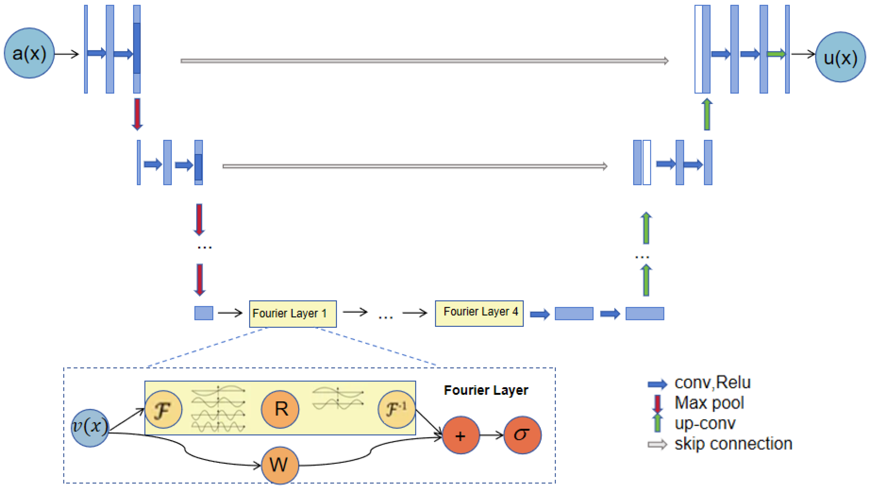
Let $s,s^{\prime }\ge 0$. Consider $F_{\theta }:H^s({\mathbb{T}}^d;{\mathbb{R}}^{d_a})\to H^{s^{\prime }}({\mathbb{T}}^d;{\mathbb{R}}^{d_u})$ as a continuous operator. Let $K\subseteq H^s({\mathbb{T}}^d;{\mathbb{R}}^{d_a})$ be a compact subset. For any $\epsilon >0$, there exists a UNO $F^{+}:H^s({\mathbb{T}}^d;{\mathbb{R}}^{d_a})\to H^{s^{\prime }}({\mathbb{T}}^d;{\mathbb{R}}^{d_u})$, continuous as an operator ($H^s\to H^{s^{\prime }}$), satisfying

$$\underset{a\in K}{sup}{∥F_{\theta }(a)-F^{+}(a)∥}_{H^{s^{\prime }}}\le \epsilon .$$

The U-Net neural network, as a classic deep learning architecture, has a unique structure. The first half is mainly responsible for feature extraction, while the second half focuses on the up-sampling operation. This structure is called the encoder–decoder structure. In this study, a Fourier neural operator with adjustable parameters is introduced As shown in the Figure 1. By skillfully integrating the feature information extracted by the U-Net neural network into the Fourier operator, the operational efficiency and solution accuracy of the algorithm can be significantly improved.

Step 1: When constructing the algorithm framework, P and Q are defined to represent the left-contracting path and the right-expanding path of the U-Net neural network, respectively:

$$\begin{array}{cc}\hfill & P:{\mathbb{R}}^{d_i}\times \Theta \to {\mathbb{R}}^{d_f}\hfill \\ \hfill & (\mathcal{P})(x,{\theta }_R)=P(u(x),{\theta }_R)\hfill \end{array}$$

(15)

Among them, $d_f$ represents the number of channels used in the neural network. Usually, the value of $d_f$ is greater than $d_i$ or $d_0$. In the actual operation, the left-contracting path (P) of U-Net is used to lift the input data to a high-dimensional channel space; then, the right-expanding path (Q) is used to project the data in the channel space to the final output space.

The left encoder network (P) has a structure similar to that of a convolutional neural network. The operation process of a given input function (a: $a:\mathbb{D}\in {\mathbb{R}}^{dA}$) includes two repeated $3\times 3$ convolution operations, a rectified linear unit (ReLU activation function), and a $2\times 2$ max-pooling layer. When performing the down-sampling operation, the algorithm’s step size is set to 2.

The convolutional layer is expressed as follows:

$$\begin{array}{c}\hfill \mathrm{Conv}(a,W,b)=a\ast W+b\end{array}$$

(16)

where $\ast$ is a convolution operation, W is the convolution kernel, and b is bias.

ReLU activation functions:

$$\begin{array}{c}\hfill \mathrm{ReLU}(z)=max(0,z)\end{array}$$

(17)

Pooling layer: The maximum pooling layer is usually used to reduce the spatial dimension and help to obtain the features of the image:

$$\begin{array}{c}\hfill \mathrm{MaxPool}(a)=\underset{\mathrm{window}}{max}(a)\end{array}$$

(18)

The result is input a into the encoder (left-contracting path (P)) of the U-net neural network. Through convolution, ReLU activation function, and max-pooling layer operations, the input is lifted to the high-dimensional channel space (${\mathbb{R}}^{d_f}$).

Step 2: Then, we introduce the nonlinear integral Fourier operator ($(\kappa (\varphi )v)(x)=$ ${\mathcal{F}}^{-1}\left(R_t·\mathcal{F}{v}_t\right)(x)$):

$$\begin{array}{c}\hfill {\mathbf{F}}_i:\{v_t:D_t\to {\mathbb{R}}^{d_{v_t}}\}\to \{v_{t+1}:D_{t+1}\to {\mathbb{R}}^{d_{v_{t+1}}}\},t\in \{0,1,2,...,T\}\end{array}$$

(19)

Four-layer integral operators and activation functions are applied to the obtained feature ($v_t:$), which is updated specifically according to the following formula:

$$\begin{array}{c}\hfill v_{t+1}(x)=\sigma (W{v}_t(x)+{\mathcal{F}}^{-1}\left(R_t(k)·\mathcal{F}{v}_t\right)(x))\end{array}$$

(20)

where $\sigma$ is an activation function and $GELU,R_t:{\mathbb{Z}}^d to {\mathbb{C}}^{d_{t+1}\times d_t}$ is a linear transformation that can handle lower Fourier patterns and filter out higher patterns ($W in {\mathbb{R}}^{to?n\times n}$ and $\varphi$) into the nucleus (${\kappa }_{\varphi }:{\mathbb{R}}^{2(d+1)}$ to ${\mathbb{R}}^{n\times n}$), corresponding to something to learn from the data.

Step 3: The result ($v_t$) is, again, input into the U-Net neural network decoder (Q), as well as deconvolution, jump connection, and other operations, helping to retain high-resolution details.

$$\begin{array}{cc}\hfill & Q:{\mathbb{R}}^{d_f}\times \Theta \to {\mathbb{R}}^{d_o}\hfill \\ \hfill & (\mathcal{Q})(x,{\theta }_Q)=Q(u(x),{\theta }_Q)\hfill \end{array}$$

(21)

Similar to the encoder, the decoder also applies the convolution and activation functions to handle the feature graph.

The updated result is input into the decoder (right-expanding path (Q)) of the U-net neural network. It is processed through operations such as deconvolution and skip connection and finally output as $u(x)$.

Step 4: The final output results and the original sample are used to calculate the loss according to the loss function; finally, the loss function is used to optimize the U-Net network and the Fourier operator to obtain the optimal parameter value.

$$\begin{array}{c}\hfill L=MS{E}_F+\lambda MS{E}_{bc/initial}.\end{array}$$

(22)

where

$$MS{E}_{bc/initial}={\displaystyle \frac{1}{N_f}}\sum _{N_f}^{i=1}{(\mu (t_0^i,x_0^i)-{\mu }_0^i)}^2 and MS{E}_F={\displaystyle \frac{1}{N_f}}\sum _{N_f}^{i=1}({\mathcal{F}}^{†}(a_0^i)-{\mathcal{F}}_{\theta }(a_0^i))$$

(23)

where ${\{t_0^i,x_0^i,a_0^i,u_0^i\}}_{i=1}^N$ represents the initial and boundary training datasets. The loss term ($MS{E}_{bc/initial}$) corresponds to constraints imposed by the initial data and boundary data.

$$\begin{array}{c}\hfill L=MS{E}_{\mathbf{F}}+{\lambda }^{\prime }MS{E}_f\end{array}$$

(24)

$$\begin{array}{c}\hfill MS{E}_f={\displaystyle \frac{1}{N_u}}\sum _{i=1}^{N_u}|f(t_f^i,x_f^i){|}^2\mathrm{and}MS{E}_{\mathbf{F}}={\displaystyle \frac{1}{N_{\mathbf{F}}}}\sum _{i=1}^{N_{\mathbf{F}}}|{\mathbf{F}}^{†}(a^i)-{\mathbf{F}}_{\theta }(a^i)|.\end{array}$$

(25)

were the set expressed as ${\{t_f^i,x_f^i\}}_{i=1}^N$ represents the collocation points for $f(t,x)$, with the loss function ($MS{E}_f$) enforcing the structural constraints imposed by equations.

The parameters of the U-Net network and the Fourier operator are optimized by the loss function to obtain the best parameter values and minimize the loss.

(a)

The complete structure of the neural operator: The entire operation process of the neural operator starts from input a. First, the input data are upgraded to a high-dimensional channel space through the U-Net encoder. Then, four layers of integral operators and activation functions are applied to deeply process the data. After that, the processed data are sent to the target dimension through the U-Net decoder; finally, u is output.

(b)

Fourier layer: The operation of the Fourier layer starts from input $\nu$. First, Fourier transform ($\mathcal{F}$) is applied to transform the data into the frequency domain. Then, a linear transformation (R) is performed on the low-frequency signals to filter out the high-frequency signals. After that, inverse Fourier transform (${\mathcal{F}}^{-1}$) is applied to transform the data back into the time domain. At the bottom, a local linear transformation (W) is also applied to further process the data.

Definition 1 (Fourier integraloperator (κ)L).

Updates are made by defining the representation of $v_t\to v_{t+1}$ as follows:

$$\begin{array}{c}\hfill v_{t+1}(x)=\sigma (W{v}_t(x)+(\kappa (a;\varphi )v_t)(x)\end{array}$$

(26)

The above formula can be seen as a combination of linear connections and nonlinear transformations and by the activation function. Nonlinear transformation ($kappa$) is implemented by a kernel integral operator:

$$\begin{array}{c}\hfill (\kappa (a;\varphi )v_t)(x)={\int }_D\kappa (x,y,a(x),a(y);\varphi )v_t(y)dy\end{array}$$

(27)

The selected kernel form is ${\kappa }_{\varphi }(x,y,a(x),a(y))={\kappa }_{\varphi }(x-y)$, formally similar to the convolution operation. Thus, it can be expressed by Fourier transform as follows:

$$\begin{array}{c}\hfill (\kappa (a;\varphi )v_t)(x)={\mathcal{F}}^{-1}(\mathcal{F}({\kappa }_{\varphi }·)\mathcal{F}(v_t))(x)\end{array}$$

(28)

A parameter matrix ($R_{\varphi }$) is introduced, which can transform the Fourier modes and filter out the higher modes. The Fourier neural operator is finally expressed as follows:

$$\begin{array}{c}\hfill (\kappa (a;\varphi )v_t)(x)={\mathcal{F}}^{-1}(R_{\varphi }·)\mathcal{F}(v_t))(x)\end{array}$$

(29)

where $\kappa \in D$, $\mathcal{F}{v}_t(\kappa )\in C^{d_v}$, and $R_{\varphi }(\kappa )\in C^{d_v\times d_v}$ are all in a function space.

4. Experiment

This section mainly uses the UNO model to solve the 1DBurgers equation, the 2DDarcy flow equation, and the 2D Navier–Stokes equation. First, we introduce the experimental configuration and the experimental parameter settings. Then, we explain the experimental effect. Finally, we solve the partial differential equation according to the model framework introduced and proposed in this chapter, comparing the merits of this model in solving partial differential equations. We obtain the solution speed, the solution result, and the error with the real solution of the model in the three equations.

4.1. Burgers Equation

In this paper, we choose the 1DBurgers equation, which is a nonlinear partial differential equation. The equations considered in this paper are formally expressed as follows:

$$\begin{array}{cc}\hfill & {\displaystyle \frac{\partial u}{\partial t}}+u{\displaystyle \frac{\partial u}{\partial x}}=\mu {\displaystyle \frac{{\partial }^{2}u}{\partial x^2}},x\in (0,1),t\in (0,1],\hfill \\ \hfill & u(x,t=0)=u_0(x),0<x<1\hfill \end{array}$$

(30)

where $u(x,t)$ is the unknown function, which depends on the time variable (t) and the spatial variable (x); $\mu \in {\mathbb{R}}_{+}$ is the viscosity coefficient; the initial condition is $u_0(x)\in L_{per}^2((0,1);\mathbb{R})$; and the boundary condition is the periodic boundary condition.

$u_0(x)$ is randomly sampled, $u_0\sim \mu ,\mu =\mathcal{N}(0,625{(-\Delta +25I)}^{-2})$, modes = 16, width = 64, and batch size = 20. The forced term = 0, the viscosity coefficient is $\mu =0.1$, the grid is $2^{13}=8192$, and other grids are directly subsampled. The network input is $a(x)=u(x,t=0)=u_0(x)$, the output is $u(x,t=1)$, we have 8192 $a(x)$ in 2048 grid samples with average sampling, neural network input dimensions of (20, 128, 2), and input neural operator dimensions of (20, 128, 64). The accuracy of the equation label determines the model accuracy; if the label accuracy is poor, the model has no sense.

The approximate solution is u, and the true solution is uacc, with an error of $O(h^2)$, $u-u_{acc}=O(h^2)$. The solver is a GPU, the error is $G(f,x,y)-u(x,y)=O(h^p)$, and a training label of G is an approximate solution.

$$\begin{array}{cc}\hfill G(f,x,y)-u_{acc}(x,y)& =G(f,x,y)-u(x,y)+u(x,y)-u_{acc}(x,y)\hfill \\ \hfill & =G(f,x,y)-u_{acc}(x,y)=\mathcal{O}(h^2)\hfill \end{array}$$

It is expected that any f = net (x, y) has G (f, x, y) satisfying the solution constraint regularization of the corresponding PDE.

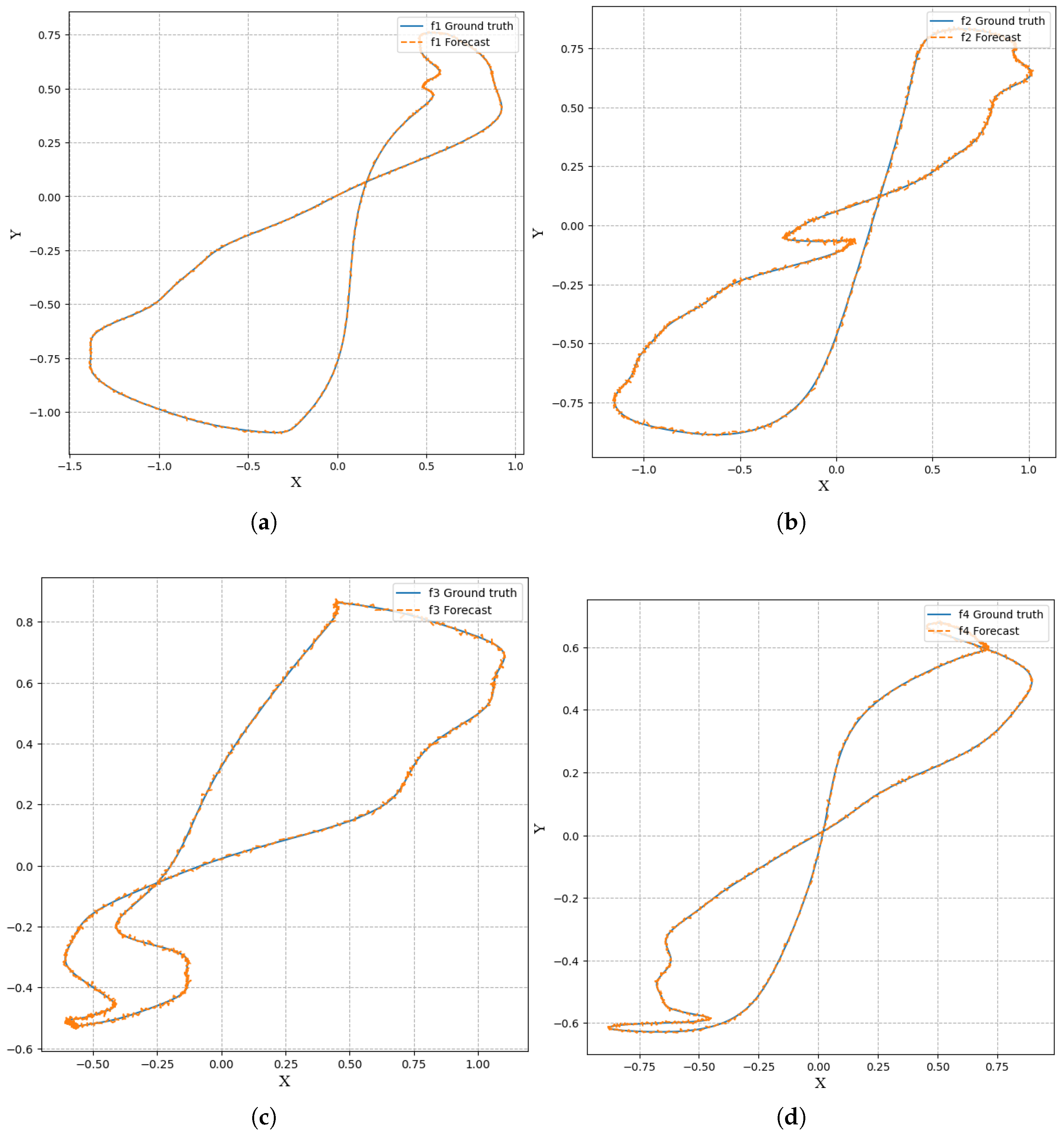
Figure 2 randomly intercepts several algorithm results from different periods, showing the error between the prediction and the true value of the algorithm, without much change to the naked eye and a good visualization effect.

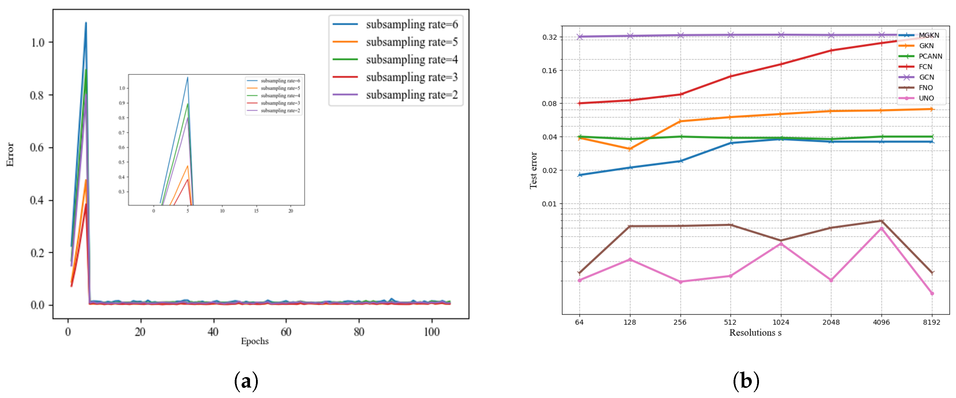
Figure 3 compares the errors as the number of iterations increases when the subsampling rate varies. We can see that when the subsampling rate is 3 and 5, the error is minimized and the algorithm is better than in other cases. It can be seen from the algorithm comparison diagram on the right of Figure 3 and

Table 1. Experiment 1 results.

Network	s = 64	s = 128	s = 256	s = 512	s = 1024	s = 2048	s = 4096	s = 8192
MGKN	0.0187	0.0223	0.0243	0.0355	0.0374	0.0360	0.0364	0.0364
GKN	0.0392	0.0325	0.0573	0.0614	0.0644	0.0687	0.0693	0.0714
PCANN	0.042	0.0391	0.0398	0.0395	0.0391	0.0383	0.0392	0.0393
FCN	0.0827	0.0891	0.1158	0.1407	0.1877	0.2313	0.2855	0.3238
GCN	0.3211	0.3216	0.3359	0.3438	0.3476	0.3457	0.3491	0.3498
FNO	0.0024	0.0063	0.0063	0.0066	0.0048	0.0060	0.0069	0.0024
UNO	0.0021	0.0032	0.0020	0.0023	0.0045	0.0021	0.0060	0.0018

that the different algorithms exhibit the ability to solve the partial differential equations in the one-dimensional Burgers equation experiment. The UNO model uses convolution to extract physical feature information. The jump connection reduces the information loss of the model. The results are more accurate than those achieved by other algorithms.

4.2. Darcy Flow

In this paper, we choose the steady-state 2DDarcy flow equation as a second-order linear elliptic partial differential equation:

$$\begin{array}{cc}\hfill -\nabla ·(a(x))\nabla u(x)& =f(x),x\in {(0,1)}^2\hfill \\ \hfill u(x)& =0,x\in \partial {(0,1)}^2,\hfill \end{array}$$

(31)

where the boundary condition is the Dirichlet boundary condition, a is the diffusion coefficient, $a(x)\in L^{\infty }({(0,1)}^2;\mathbb{R})$, $u\in H_0^1({(0,1)}^2;\mathbb{R})$ is the solution, and the external force is $f(x)\in H^{-1}({(0,1)}^2;\mathbb{R})$.

We processed the dataset as follows: first, $\mu ={\psi }_{\#}\mathcal{N}(0,625{(-\Delta +9I)}^{-2})$ is a probability measure with zero Neumann boundary conditions on LaPraaca, where $\forall x\ge 0,\psi (x)=12$ and $\forall x<0,\psi (x)=3$. The external force is fixed to be $f(x)=1$. The coefficient ($a(x)$) was sampled from $\mu$, and the solution (u) was obtained using the traditional finite element method on the $64\times 64$ and $256\times 256$ grids in Matlab. Datasets with different resolutions can be generated by downsampling. We parameterized a two-dimensional Fourier neural operator consisting of four Fourier layers with 20 frequencies per channel and width = 64.

The loss function can be written in the following form:

$$MS{E}_f=-\nabla ·(a(x))\nabla u(x)-f(x).$$

In the experimental section, the FNO model, ResNet model, TFNET model, and UNO model were used to solve the 2DDarcy flow equation.

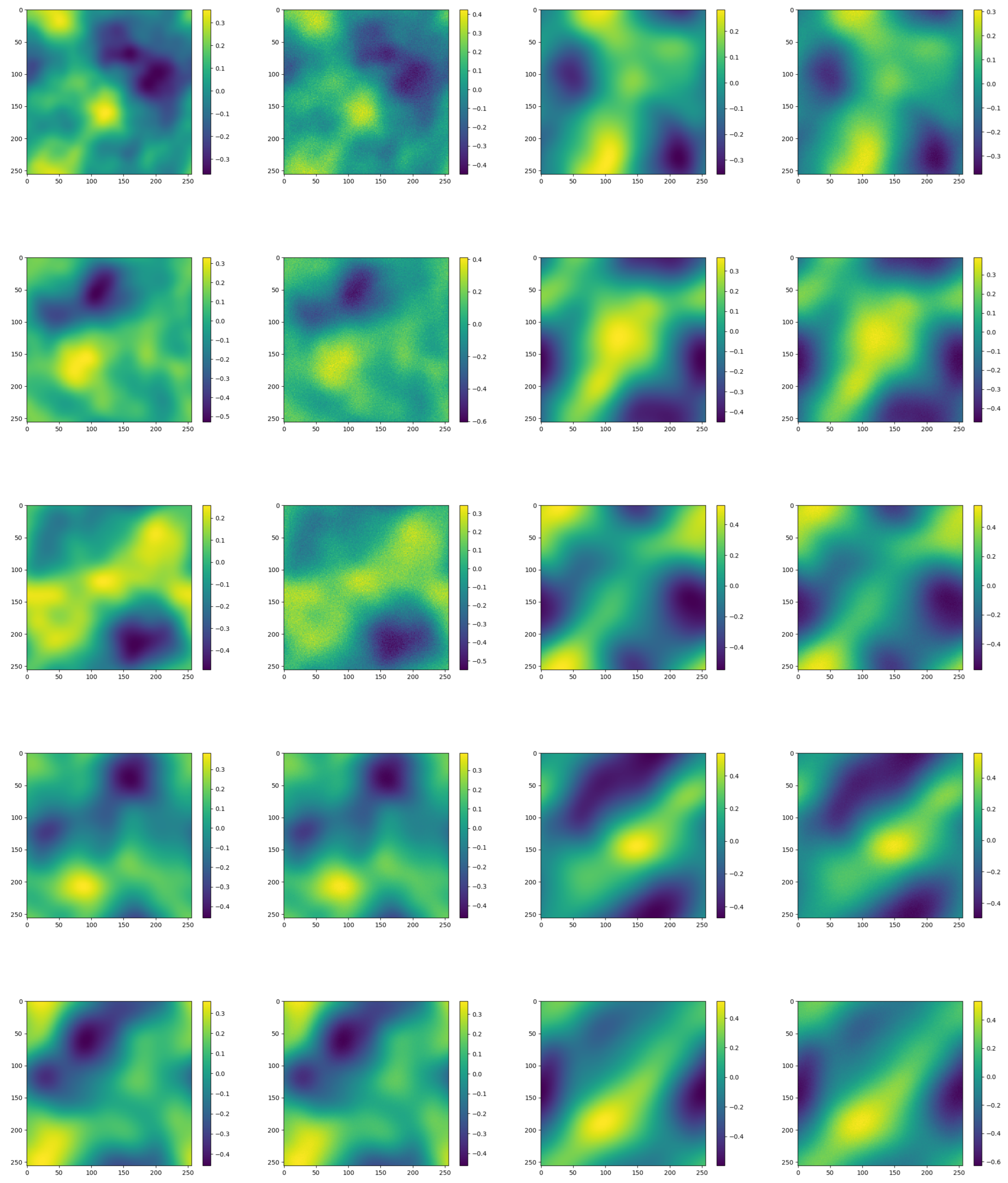
The true and model solutions of the equations and their errors are shown in Figure 4.

Figure 4 shows the contrast between the true and predicted values from 1 s to 5 s and the error situation per second.

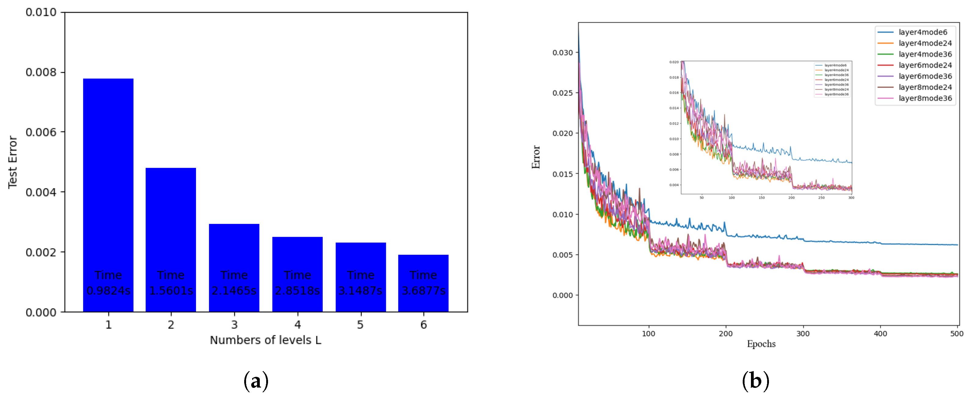
Figure 5 (left) shows that the number of Fourier neural operator layers varies. When the number of Fourier neural operator layers is 1, it takes the least time and the test error is the largest. When the number of levels increases, the duration increases, but the test error is reduced. Three, four, or five layers are most reasonable, depending on the situation. Here, we consider a four-layer Fourier operator. The right image introduces the effect of different numbers of Fourier neural operator layers and the filtered models on the algorithm error as the number of iterations increases. As the number of iterations increases, the error becomes smaller. For the four-layer Fourier neural operator with 24 filtered-out models, the effect is better, and the performance is better. Then, the algorithm model selects the four-layer Fourier neural operator.

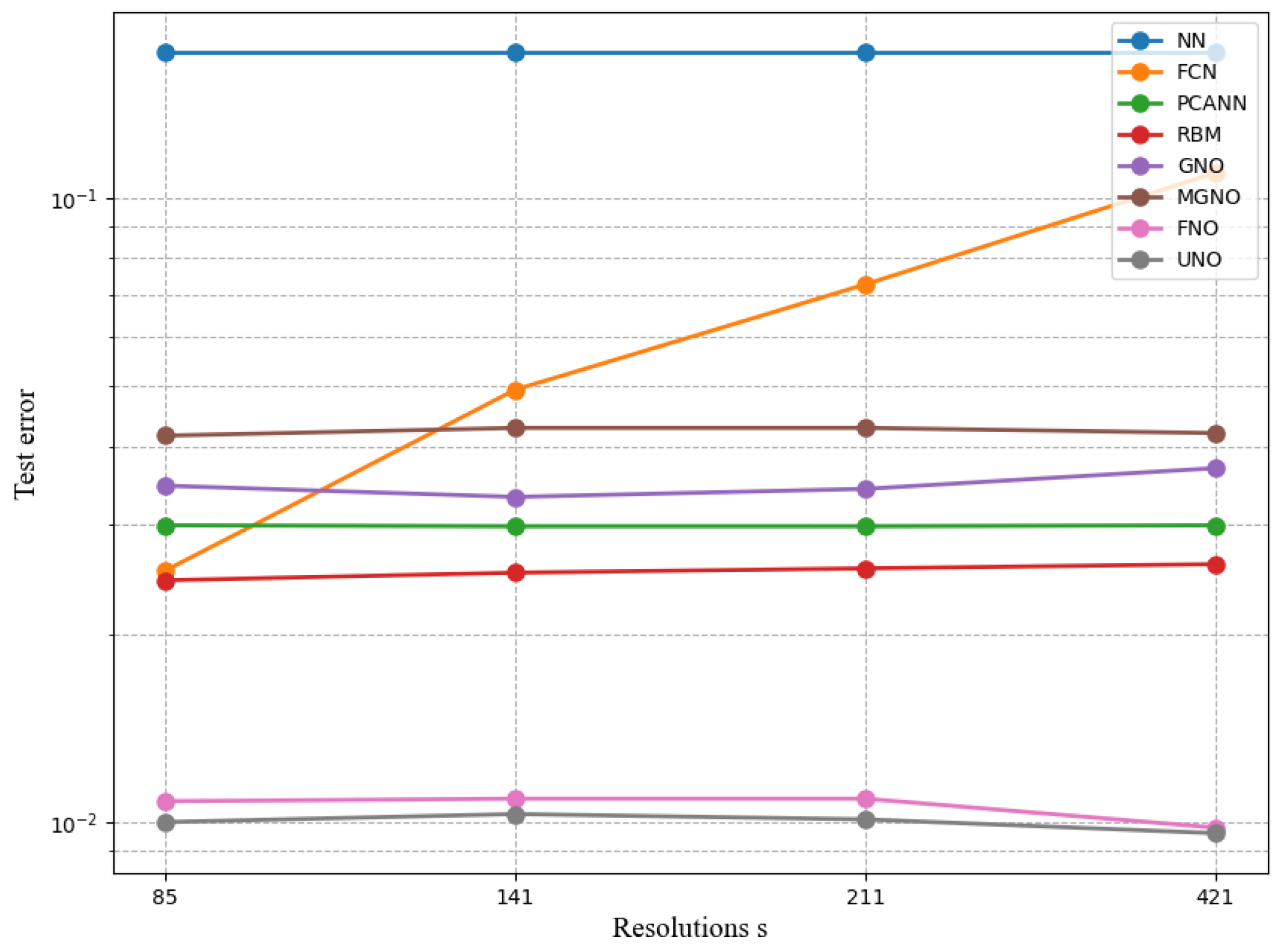
It can be seen from Figure 6 and

Table 2. Experiment 2 results.

Network	s = 85	s = 141	s = 211	s = 421
NN	0.1716	0.1716	0.1716	0.1716
FCN	0.0253	0.0493	0.0727	0.1097
PCANN	0.0299	0.0298	0.0298	0.0299
RBM	0.0244	0.0251	0.0255	0.0259
GNO	0.0346	0.0332	0.0342	0.0369
MGNO	0.0416	0.0428	0.0428	0.0420
FNO	0.0122	0.0124	0.0125	0.0099
UNO	0.0108	0.0109	0.0109	0.0098

that when different algorithms contrast error maps at resolutions of $85\times 85$, $141\times 141$, $211\times 211$, and $421\times 421$, UNO has lower and more stable error loss values compared to the most similar FNO algorithm.

4.3. Navier–Stokes Equation

In this paper, the incompressible fluid equation of motion, namely the two-dimensional Navier–Stokes equation is chosen for experiments. The equation used in this paper is expressed as follows:

$$\begin{array}{cc}\hfill {\partial }_{t}w(x,t)+u(x,t)\nabla w(x,t)& =\nu \nabla w(x,t)+f(x),x\in {(0,1)}^2,\hfill \\ \hfill \nabla u(x,t)& =0,x\in {(0,1)}^2,t\in [0,T]\hfill \\ \hfill w(x,t=0)& =w_0(x),x\in \Omega .\hfill \end{array}$$

(32)

where $u(x,t)$ is the fluid velocity; ∇ represents the gradient operator; $u_0(x)\in L_{per}^2((0,1);\mathbb{R})$ represents the initial condition, namely the initial vorticity; $\nu \in {\mathbb{R}}_{+}$ represents the viscosity coefficient; and $f(x)\in L_{per}^2((0,1);\mathbb{R})$ for the external force acting on the fluid. This article sets the external force to $f(x)=0.1(sin(2\pi (x_1+x_2))+cos(\pi (x_1+x_2)))$.

The experimental scenario is the vorticity form of the sticky, non-compresable NS equation in two dimensions. The vorticity field is simplified by directing on x and y to obtain the velocity field (u) and v using the NS equation. Using the vorticity equation as the loss function, the output layer of the neural network needs a neuron to represent w, and the automatic differentiation only needs to guide this one variable, which is often less difficult to optimize. This scenario inputs the vorticity field variable at time t at [0, 10) to the FNO model, with resolutions of $64\times 64$ and $256\times 256$, that is, to generate the dataset, the initial vorticity condition ($w_0$) is sampled randomly from the distribution of $w_0\sim \mu ,\mu =\mathcal{N}(0,7^{3/2}{(-\Delta +49I)}^{-2.5})$, with periodic boundary conditions. The input variable dimensions are [64, 64, 10] and [256, 256, 10]. It is hoped that the FNO model can output the value of the vorticity field at time $t>10$, that is, learn the evolution relationship of the vorticity time series and realize a model similar to the time-series prediction.

The loss functions are defined as follows:

$$\begin{array}{c}\hfill MS{E}_f={\partial }_{t}w(x,t)+u(x,t)\nabla w(x,t)-\nu \nabla w(x,t)+f(x)\end{array}$$

Figure 7 shows images of true and predicted values from 1 s to 10 s, from top to bottom. As can be seen from the image comparison per second, the visualization results are relatively consistent, with minimal error.

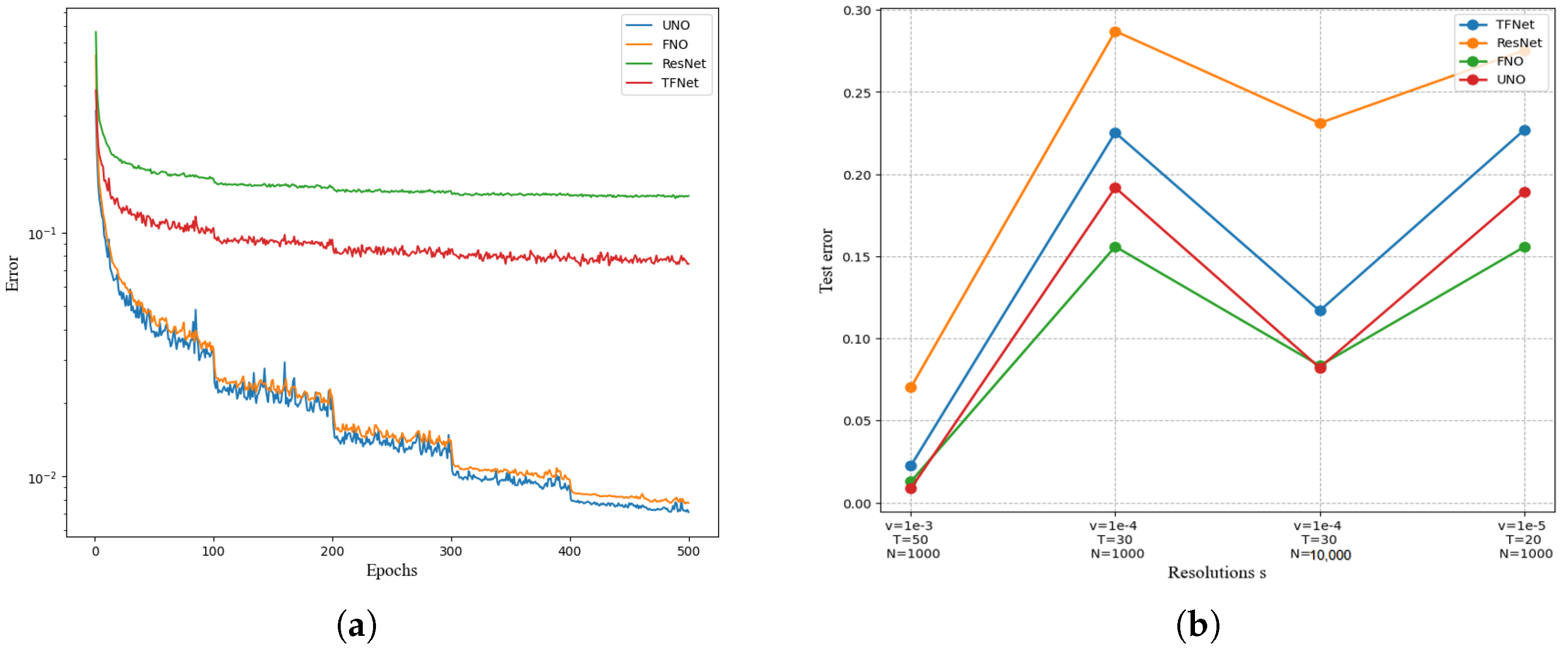
As shown in Figure 8, FNO and UNO achieve the best results. By comparing time and data points, suitable algorithms are selected. The errors of the UNO and FNO algorithms continue to decrease steadily with the number of iterations, with great advantages compared with other models. The error of the UNO algorithm drops faster, with an obvious decreasing process at 100, 200, 300, and 400, showing a continuous jitter decreasing trend, with obvious advantages in solving the equation. The RENET and TFNET models are less effective, and compared with UNO and FNO, the curves are relatively smooth and the errors are larger during iteration. Figure 8 and

Table 3. Experiment 3 results.

Network	Total Number of Parameters	Duration of Each Round of Training	v = 1 $\times {10}^{-3}$ T = 50 N = 1000	v = 1$\times {10}^{-4}$ T = 30 N = 1000	v = 1$\times {10}^{-4}$ T = 30 N = 10,000	v = 1$\times {10}^{-5}$ T = 20 N = 1000
UNO	414,517	38.99 s	0.0128	0.1879	0.0834	0.1856
FNO	655,853	45.80 s	0.0135	0.1551	0.0835	0.1524
Re sNet	266,641	78.47 s	0.1716	0.2871	0.2311	0.2753
TF-Net	7,451,724	47.21 s	0.0225	0.2253	0.1168	0.2268

also compares the experimental errors of UNO and FNO, RENET, and TFNET on the dataset. The figure shows N = 10,000 data points and T = 50. When the viscosity coefficient is $1\times {10}^{-3}$, the UNO error is the smallest, and UNO has higher accuracy. When the number of data points is N = 1000, UNO is worse than FNO, but when the number of data points increases to N = 10,000, the UNO error is the lowest among the compared algorithms, and 400.

5. Conclusions

This paper proposes an innovative method based on the combination of U-Net neural networks and Fourier neural operators, aiming to improve the accuracy and efficiency of solving partial differential equations (PDEs). By integrating the unique encoder–decoder structure and skip connections of U-Net with the deep feature processing capabilities of Fourier transform in the frequency domain, the method fully leverages the strengths of U-Net in spatial feature extraction and the capabilities of Fourier transform in frequency-domain feature processing. This combination not only preserves spatial details but also captures both high-frequency and low-frequency characteristics of PDE solutions through frequency-domain analysis, thereby significantly enhancing solution accuracy. Experimental results demonstrate that, compared to traditional methods, this approach performs exceptionally well in various complex PDE-solving tasks, achieving high accuracy. While the method reduces reliance on large-scale datasets, high-quality datasets remain crucial for the training of the model when dealing with complex physical systems. Future research could explore ways to further improve the model’s generalization ability in data-scarce scenarios.