Effects of Diffusion and Delays on the Dynamic Behavior of a Competition and Cooperation Model

Abstract

This study investigates a model of competition and cooperation between two enterprises with reaction, diffusion, and delays. The stability and Hopf bifurcation for variants with two, one, and no delays are considered by examining a system of delay ODE equations analytically and numerically, applying the Galerkin method. A condition is obtained that helps characterize the existence of Hopf bifurcation points. Full maps of stability analysis are discussed in detail. With bifurcation diagrams, three different cases of delay are shown to determine the stable and unstable regions. It is found that when ${\tau }_i>0$, there are two different stability regions, and that without a delay (${\tau }_i=0$), there is only one stable region. Furthermore, the effects of delays and diffusion parameters on all other free rates in the system are considered; these can significantly affect the stability areas, with important economic consequences for the development of enterprises. Moreover, the relationship between the diffusion and delay parameters is discussed in more detail: it is found that the value of the time delay at the Hopf point increases exponentially with the diffusion coefficient. An increase in the diffusion coefficient can also lead to an increase in the Hopf-point values of the intrinsic growth rates. Finally, bifurcation diagrams are used to identify specific instances of limit cycles, and 2-D phase portraits for both systems are presented to validate all theoretical results discussed in this work.

1. Introduction and Preliminaries

There has recently been considerable interest from mathematicians in a variety of nonlinear systems that can accurately describe phenomena in our daily lives, including in population ecology [1,2,3], animal behavior [4,5,6], health [7,8,9], chemistry [10,11], and business and economics [12,13,14,15,16]. In recent decades, a significant stream of literature has focused on examining enterprises and their development, growth trends, market positions, and relationships with each other in the business ecosystem [17,18,19]. These studies have analyzed various aspects of competition and cooperation between enterprises, and have played a crucial role in improving our understanding of both individual businesses and the wider economy.

The significance of the dynamic relationships between enterprises has been considered and modeled using both ODEs or PDEs. A variety of tools have been used to explore aspects of their behavior, such as attractivity, persistence, Hopf bifurcations, and equilibrium stability, including systems with delays; see [15,20,21,22] and references therein. A standard model of competition and cooperation for two enterprises was analyzed in [23]. The existence of a periodic solution was shown using the continuation theorem of coincidence degree theory. This system is defined by the following equations:

$$\begin{array}{c}{\displaystyle \frac{d{u}_1}{dt}}=r_1{u}_1\left(t\right)\left[1-{\displaystyle \frac{u_1\left(t\right)}{K_1}}-{\displaystyle \frac{\alpha {(u_2\left(t\right)-c_2)}^2}{K_2}}\right],\hfill \\ {\displaystyle \frac{d{u}_2}{dt}}=r_2{u}_2\left(t\right)\left[1-{\displaystyle \frac{u_2\left(t\right)}{K_2}}+{\displaystyle \frac{\beta {(u_1\left(t\right)-c_1)}^2}{K_1}}\right].\hfill \end{array}$$

(1)

In this model, $u_1$ and $u_2$ refer to the output of two enterprises at time t and location x, $r_1$ and $r_2$ represent the intrinsic growth rates for their output, and $K_1$ and $K_2$ are their load capacities in an unrestricted natural market (the carrying capacity of the market under unlimited conditions). In addition, $\alpha$ and $\beta$ are coefficients representing the degrees of competition or cooperation practiced by the two enterprises, and $c_1$ and $c_2$ are their initial production.

Analytical and theoretical studies of an economic system can contribute to our understanding of dynamic relationships among several enterprises, and can also have an important impact on the business ecological environment. Therefore, analyzing interactions between enterprises is of great significance in helping those enterprises understand their situation. Here, we assume that the two enterprises are constantly engaged in competition and cooperation, that when an enterprise suffers damage from competition, the other one can benefit, and that they can both gain advantages through cooperation. Meanwhile, the periodic yield of each business can also have a significant effect. We also assume time delays for the competition and cooperation in system (1). The presence of time delays can have a large impact on the dynamics of a system. In ODE models, this can cause the loss of stability and can induce various oscillations and periodic solutions through Hopf bifurcations. Delay can also affect the stability of steady states and lead to the formation of multiple equilibria and limit cycles; for example, see [7,12,19]. Therefore, we are interested in adding two time delays to the two-enterprise system (1), as in [15,18]. Such time delays always exist in the cooperation and competition between different enterprises and have important economic consequences for their development, as we shall see in this work. Hence, the new form of the ODEs, including the two delays, is as follows:

$$\begin{array}{c}{\displaystyle \frac{d{u}_1}{dt}}=r_1{u}_1\left(t\right)\left[1-{\displaystyle \frac{u_1\left(t\right)}{K_1}}-{\displaystyle \frac{\alpha {(u_2(t-{\tau }_2)-c_2)}^2}{K_2}}\right],\hfill \\ {\displaystyle \frac{d{u}_2}{dt}}=r_2{u}_2\left(t\right)\left[1-{\displaystyle \frac{u_2\left(t\right)}{K_2}}+{\displaystyle \frac{\beta {(u_1(t-{\tau }_1)-c_1)}^2}{K_1}}\right],\hfill \end{array}$$

(2)

where ${\tau }_1>0$ is the delay with which $u_1$ affects $u_2$, and ${\tau }_2>0$ is the delay from $u_2$ to $u_1$. We can rewrite this system by letting ${\delta }_1=r_1/K_1$, ${\delta }_2=r_2/K_2$, ${\mu }_1=\alpha r_1/K_2$, and ${\mu }_2=\beta r_2/K_1$, and incorporating the Laplacian operator (the diffusion effect). Diffusion and delays can have significant impacts on the behavior of this system, potentially leading to the formation of spatial patterns in the dynamics, which can affect the stability of the system and the occurrence of bifurcations. Thus, the nonlinear reaction–diffusion system for a two-enterprise model with two time delays can be expressed as follows [22]:

$$\begin{array}{c}{\displaystyle \frac{\partial u_1}{dt}}-d_1{\displaystyle \frac{\partial u_1^2}{\partial x^2}}=u_1\left(t\right)\left(r_1-{\delta }_1{u}_1\left(t\right)-{\mu }_1{(u_2(t-{\tau }_2)-c_2)}^2\right),\hfill \\ {\displaystyle \frac{\partial u_2}{dt}}-d_2{\displaystyle \frac{\partial u_2^2}{\partial x^2}}=u_2\left(t\right)\left(r_2-{\delta }_2{u}_2\left(t\right)+{\mu }_2{(u_1(t-{\tau }_1)-c_1)}^2\right),\hfill \end{array}$$

(3)

where ${\mu }_1$ is the consumption coefficient from the enterprise with the output $u_2$ to the enterprise with the output $u_1$, and ${\mu }_2$ indicates the transformation coefficient from the enterprise with the output $u_1$ to the enterprise with the output $u_2$. In addition, $d_1$ and $d_2$ are the diffusion rates due to the other species in the model. Both ${\delta }_1$ and ${\delta }_2$ are positive rates representing inter-species competition. Further, we consider Dirichlet boundary conditions, as follows:

$$\begin{array}{c}{u}_1(x,t)=u_2(x,t)=0\mathrm{at}x=\pm 1\mathrm{and}t=0,\\ u_1=u_2=u_{ss}\mathrm{when}-{\tau }_1<t\le 0\mathrm{and}-{\tau }_2<t\le 0.\end{array}$$

(4)

This system is open and at the center of the domain $x=0$, a zero-flux boundary condition is assumed. The boundary condition at the center of the domain is a symmetry condition; an identical reservoir is located at $x=-1$. Hence, it is an open system; a permeable boundary at $x=1$ is assumed in the reactor, which is joined to a reservoir in which $u_1$ and $u_2$ have zero concentrations. In addition, the constant $u_{ss}>0$ represents the model’s concentrations $u_1$ and $u_2$ for $t\in (-{\tau }_1,0)$ and $t\in (-{\tau }_2,0)$ (the changing values of the initial concentration condition do not affect the solutions or stability regions). The use of spatial diffusion with zero-flux boundary conditions in this system is motivated by the fact that enterprises located in the center of a city typically serve as centers of activity for manufacturing, information, transportation, trade, services, and decision-making. This tends to attract production from surrounding regions and spread production factors to those areas. In particular, as industrial economic expansion in the central region matures, the effect of diffusion continues to grow [12,22,24,25]. This is the economic rationale for choosing this type of spatial diffusion in the system.

The dynamics of a two-species, two-enterprise interaction model with time delays have been discussed in various scientific contexts. For example, in [15,19], a two-species competition–cooperation system for two enterprises with time delays was studied. These works demonstrated the impact of time delays on bifurcations and the stability of the positive equilibrium. In addition, the authors of [26] studied the same dynamical system as in [15], with two small delays. They theoretically found a simple approach to derive approximate roots of the characteristic equation. In [18], the dynamic development of a two-enterprise system with time delay was investigated. The stability of the unique positive equilibrium and the existence of a Hopf bifurcation were analyzed via normal form theory and the center manifold theorem. The study also found that the positive equilibrium is locally asymptotically stable when the value of the time delay is less than a certain critical value. However, as the delay time increases beyond this critical value, the positive equilibrium becomes unstable. A competition–cooperation enterprise cluster model with a core–satellite structure was studied in [17]. The researchers found that there is an upper bound on both the core and satellite enterprise outputs. This upper bound not only depends on the production ability of each enterprise individually, but also on the production ability of the two satellite enterprises. Many further studies on the stability and bifurcations of two-enterprise models with delays can be found in the literature, including in [20,21,24,27].

The literature includes a few research works focused on the two-enterprise interaction model with diffusion and delay. In [22], a two-enterprise interaction model with diffusion and delay was studied using normal form theory and center manifold reduction of PDEs. The study aimed to determine the direction of any Hopf bifurcations and the stability of the periodic outcomes. The researchers found that as the time delay passes through a critical value, the model transitions from a stable to an unstable state. Numerical schemes were also used to validate the analytical solutions obtained. As yet, in the existing literature above, it appears that there is a gap regarding the influence of the two delay and diffusion coefficient values on the stability and bifurcations of the two-species model. The reason for this is that the majority of existing and current research has focused on delay ODE systems [15,17,19,20,21] rather than PDE models. A few studies have also determined theoretical outputs for PDE models, but none of them covered the full effect of two delay and diffusion values or provided full theoretical and numerical analyses. Therefore, it is of significant practical importance to analyze the dynamic properties of this system, which may help in understanding the evolution and behavior of markets and facilitate the implementation of appropriate regulatory strategies on the timing of decision-making. Furthermore, to gain a better understanding of enterprises’ market positions, it is necessary to discuss the dynamic interactions between enterprises and evaluate the impacts of diffusion and delay parameters. Hence, the main purpose of this paper is to study the impact of the diffusion coefficient, with two different delay terms, on the model of competition and cooperation between two enterprises. This research has several objectives:

(i)

To investigate the effects of three different cases of delay terms on stability and Hopf bifurcation areas, in order to understand how these delays interact with the diffusion parameters, growth rates, and other free rates in the model.

(ii)

To illustrate the theoretical properties of the DDEs using the Galerkin method, which provides accurate approximate solutions for delay PDEs.

(iii)

To explore analytically a condition for the existence of Hopf bifurcation points.

(iv)

To construct bifurcation diagrams, limit cycle plots, and 2-D phase portraits, in order to verify the theoretical findings.

(v)

To explain how these results relate to real-world scenarios and the potential benefits of applying them to practical situations.

Section 2 sets out the methodology used to develop the theoretical framework. In addition, we present the theoretical conditions that can aid in identifying Hopf points. In Section 3, we produce Hopf bifurcation maps to analyze stability, considering both theoretical and numerical outputs. This section is divided into three subsections, which show how the three different delay sources interact with the other free parameters in the system. In Section 4, bifurcation diagrams are constructed for the delay ODE and PDE models, and the long-term behavior is studied numerically to demonstrate the analytical solutions and gain further insight into their properties.

2. Methodology and Framework

2.1. The Galerkin Technique

Theoretical results are significant for developing an understanding of PDE systems. However, for some systems, it has proven difficult to obtain reliable results that explain their behavior and the possibility of linking them to real phenomena. In this section, we consider the Galerkin technique, an effective method for deriving approximate solutions to various PDE models [11,28]. Galerkin’s method uses orthogonality to the base function collections, to convert PDE into ODE or DDE systems. This technique is important and useful, and it presents a temporal–spatial separation and examines a spatial form of profile density. This technique outputs a system of ODEs or DDEs that approximates a nonlinear PDE or DPDE system. After describing this technique, we will discuss how to determine an analytical framework that yields analytical results for stability and Hopf bifurcations.

The Galerkin approach has been extensively applied to a wide range of complex real-world systems, such as viral infection [1,7], Nicholson’s blowflies [5], the business cycle [12], classes of delay logistic systems [2], the Brusselator system [29], limited-food systems [30], the Gray–Scott system [11], the Belousov–Zhabotinsky system [31], and, recently, advection–competition systems [32]. The results of these studies generally show a strong agreement between theoretical and numerical results, and provide valuable information relevant to real-world applications. The Galerkin method has been applied to several applications in one-, two-, or higher-dimensional domains; for an example, see [5,31]. However, higher-dimensional problems generally are a more severe test of the semi-analytical method, producing slightly larger errors, see [33], and may also need more time to obtain excellent results.

As an example, a recent work [7] investigated a diffusive viral infection system with a delayed immune response in a 1-D domain. The Galerkin technique was applied, and steady-state and bifurcation conditions were identified. This study demonstrated that the time delay of the cytotoxic T lymphocyte response and the diffusion factor had a significant effect on the stability regions. In addition, bifurcation maps with limit cycles were plotted and compared between analytical and numerical results. An excellent agreement was found in all examples and cases. In another application [34], both analytical and numerical solution schemes were used to analyze a diffusive and delayed Schnakenberg model. Steady-state and bifurcation solutions were found, and it was observed that the delay time of maturation, gene expression, and diffusion parameters had a strong influence on stability and the bifurcation regions. In [35], the Galerkin approach was used to study a diffusive Selkov–Schnakenberg system. The study included stability analyses and bifurcation maps, which were compared with numerical simulations. In [12], analytical and numerical simulations of an economic system called the Kaldor–Kalecki model were obtained. Delay terms in the gross product and capital stock functions were considered. The diffusion and delay parameters were shown to have various effects on the stability of the business cycle, with the Hopf zone decreasing as the delay in investment increased.

To expand the PDE model into an ODE system, we begin by implementing the following trial expression functions:

$$\begin{array}{c}{u}_1(x,t)=u_{11}\left(t\right)cos({\displaystyle \frac{1}{2}}\pi )+u_{12}\left(t\right)cos({\displaystyle \frac{3}{2}}\pi ),\hfill \\ u_2(x,t)=u_{21}\left(t\right)cos({\displaystyle \frac{1}{2}}\pi )+u_{22}\left(t\right)cos({\displaystyle \frac{3}{2}}\pi ),\hfill \\ u_1(x,t-{\tau }_1)=u_{11}(t-{\tau }_1)cos({\displaystyle \frac{1}{2}}\pi )+u_{12}(t-{\tau }_1)cos({\displaystyle \frac{3}{2}}\pi ),\hfill \\ u_2(x,t-{\tau }_2)=u_{21}(t-{\tau }_2)cos({\displaystyle \frac{1}{2}}\pi )+u_{22}(t-{\tau }_2)cos({\displaystyle \frac{3}{2}}\pi ).\hfill \end{array}$$

(5)

The expressions applied here are built and chosen as $u_1(x,t)=u_{11}+u_{12}$ and $u_2(x,t)=u_{21}+u_{22}$, this refers to the concentration profile at the cell centers (i.e., where $x=0$). They satisfy the boundary conditions (4) of the PDE system. The free parameters in this model are then found by calculating the rates of the delay PDE equations. Then, we weight each equation in (3) using the two trial functions $cos({\displaystyle \frac{1}{2}}\pi )$ and $cos({\displaystyle \frac{3}{2}}\pi )$. Therefore, a system of four ODEs, as in (A1), who named analytical solutions for the two-term, is shown in the Appendix A. The reason for the truncation to the two terms in (5) is that it simplifies the trial functions, while still providing good agreement with the numerical simulation scheme of the delay PDE equations. Moreover, the results for the one-term trial function can be obtained by setting $u_{12}=u_{22}=0$ and $u_{12\tau }=u_{22\tau }=0$ in the ODE system (A1).

2.2. The Dynamical Theoretical Formulations

In this subsection, we analytically explore a condition for the existence of stability. This framework provides a condition that helps us to examine the Hopf bifurcation points analytically for system (A1), and hence to analytically construct diagrams for stability analysis. Moreover, the analytical outcomes of the delay ODE system (A1) are compared against numerical simulations of the delay PDE model (3).

The Hopf bifurcation point is a critical threshold, where limit cycles (periodic oscillation) emerge near an equilibrium steady-state point and the model transitions between stable and unstable states. This transition is associated with a conjugate eigenvalue pair crossing the imaginary axis [36,37,38]. The Hopf bifurcation point can be determined from the Taylor series, which can be truncated to create a polynomial approximation of the system at the steady state by assuming that

$$\begin{array}{c}{u}_{1i}=u_{1is}+ϵB_1{e}^{-\lambda t},u_{1i\tau }=u_{1is}+ϵB_1{e}^{-\lambda t}{e}^{\lambda {\tau }_1},\\ u_{2i}=u_{2is}+ϵB_2{e}^{-\lambda t},u_{2i\tau }=u_{2is}+ϵB_2{e}^{-\lambda t}{e}^{\lambda {\tau }_2},\\ \mathrm{where}i=1,2\mathrm{and}ϵ\ll 1.\end{array}$$

(6)

The equations for $u_{1i}$, $u_{2i}$, $u_{1i\tau }$, and $u_{2i\tau }$ from (6) can be substituted into (A1) and linearized around the steady-state point [1,11,34] to obtain the characteristic equation at the equilibrium points. Consequently, the associated Jacobian matrix $J_i$ can be expressed as

$$Jac=\left[\begin{array}{cccc}{\displaystyle \frac{\partial F_1}{\partial u_{11}}}-\lambda & {\displaystyle \frac{\partial F_1}{\partial u_{21}}}& {\displaystyle \frac{\partial F_1}{\partial u_{12}}}& {\displaystyle \frac{\partial F_1}{\partial u_{22}}}\\ {\displaystyle \frac{\partial F_2}{\partial u_{11}}}& {\displaystyle \frac{\partial F_2}{\partial u_{21}}}-\lambda & {\displaystyle \frac{\partial F_2}{\partial u_{12}}}& {\displaystyle \frac{\partial F_2}{\partial u_{22}}}\\ {\displaystyle \frac{\partial F_3}{\partial u_{11}}}& {\displaystyle \frac{\partial F_3}{\partial u_{21}}}& {\displaystyle \frac{\partial F_3}{\partial u_{12}}}-\lambda & {\displaystyle \frac{\partial F_3}{\partial u_{22}}}\\ {\displaystyle \frac{\partial F_4}{\partial u_{11}}}& {\displaystyle \frac{\partial F_4}{\partial u_{21}}}& {\displaystyle \frac{\partial F_4}{\partial u_{12}}}& {\displaystyle \frac{\partial F_4}{\partial u_{22}}}-\lambda \end{array}\right].$$

(7)

The eigenvalues $\lambda$ of the Jacobian matrix indicate the points in the system where small perturbations can arise. To obtain the characteristic polynomial equation, we set $\lambda =i\omega$ and split the polynomial into its real part ℜ and imaginary part ℑ. The identification of the bifurcation point involves assuming the following condition:

$$F_1=F_2=F_3=F_4=\Re =\Im =0.$$

(8)

We use the CN-FDM and RK4 methods [39,40] to obtain numerical solutions for the delay PDEs (3) and delay ODEs (A1), respectively. The spatial and temporal discretizations applied in this work are $\Delta x=\Delta t=5\times {10}^{-3}$, and positive initial parameter values $u_{1is}=u_{2is}=0.1$ are selected in all numerical investigations. The numerical simulations in this work were performed using Maple 15 [41].

3. Stability and Bifurcation Analysis

This section uses time delay as a bifurcation and control parameter to explore the stability of the system. Three different cases of the time delay ${\tau }_i$ are examined: ${\tau }_1={\tau }_2=0$ (with no delay), ${\tau }_1={\tau }_2\ne 0$ (with one delay), and with two delays ($0<{\tau }_1\ne {\tau }_2>0$). Further, bifurcation maps are plotted to illustrate the impact of each delay time on diffusion, growth rates, and other free parameters in the model (${\mu }_i$, ${\delta }_i$, $r_i$, $d_i$, and $c_i$). Moreover, the theoretical outcomes of the delay ODE system (A1) are compared against numerical simulations of the delay PDE model (3). The Hopf bifurcation regions are determined and plotted for both the theoretical ODE outputs (A1) and the simulations of the PDEs (3), and the outcomes are compared. We also plot diagrams of the stability and Hopf bifurcation regions and provide some numerical simulation examples. Additionally, we examine the impact of the diffusion coefficient rates $d_i$ on all the free rates in the system and their influence on the stability regions.

3.1. Hopf Bifurcation with No Delay (${\tau }_1={\tau }_2=0$)

Figure 1a,b show the steady states for the two enterprises $u_1$ and $u_2$ plotted against the intrinsic growth rate $r_1$. The steady-state curves are found by letting both delay times tend to zero (${\tau }_1={\tau }_2=0$) in each expression for $u_{1i\tau }$ and $v_{2i\tau }$ in the ODE system (A1), as in [1,7,34]. The analytic results are shown with dashed black curves, whereas the red crosses show the numerical outcome of the PDE model, with $r_2=3$, $d_i=0.01$, ${\mu }_i=0.2$, $\tau =0$, $c_i=0.1$, and ${\delta }_i=3$. It can be seen that, as the intrinsic growth rate $r_1$ increases, the densities of both enterprises $u_1$ and $u_2$ increase slowly across the whole domain examined. In the absence of a delay term, no Hopf bifurcation occurs. As a result, all two-enterprise systems have asymptotically stable outputs; these results are similar to those previously discussed in [15,18,19]. Furthermore, Figure 1c,d show the steady-state spatial profiles $u_1$ and $u_2$ for $r_1=8$, which display a single central peak. This occurs at $(u_1,u_2)=(2.99,1.66)$ in the analytic solution, and at $(u_1,u_2)=(2.96,1.64)$ according to the numerical simulation results, which agree within about $1\%$.

Figure 2a,b depict the behavior of steady-state lines for both enterprises $u_1$ and $u_2$ with the growth rate $r_2$. The curves are identified in Figure 1c,d, showing the steady-state spatial profiles $u_1$ and $u_2$ for $r_1=8$, which display a single central peak, with the parameters set as $r_1=5$, $d_i=0.01$, ${\mu }_i=0.2$, $\tau =0$, $c_i=0.1$, and ${\delta }_i=3$. The results depicted in Figure 1c,d show the steady-state spatial profiles $u_1$ and $u_2$ for $r_1=8$, which display a single central peak (a), and show a transition from a state of high concentration conversion to a state of minimal conversion for the growth rate $r_2$ in the case of enterprise $u_1$. However, Figure 1c,d show the steady-state spatial profiles $u_1$ and $u_2$ for $r_1=8$, which display a single central peak (b), and the growth rate $r_2$ goes from minimal to high concentration for the enterprise $u_2$. Figure 1c,d show the steady-state spatial profiles $u_1$ and $u_2$ for $r_1=8$, which display a single central peak c,d, showing the behavior of steady-state profiles for $u_1$ and $u_2$. Figure 1c,d show the steady-state spatial profiles $u_1$ and $u_2$ for $r_1=8$, which display a single central peak, both cases feature a single, central peak at $x=0$, which occurred at $(u_1,u_2)=(1.07,3.97)$ for the ODEs and at $(u_1,u_2)=(1.02,3.88)$ for the PDE numerical simulations. In general, there was excellent agreement between the analytical system and the PDE model, with a relative discrepancy under $5\%$. It can be seen that the two growth rates led to a substantially different production for both enterprises, and this may lead to reduced capacity fluctuations. These findings can aid in promoting the stable development of enterprises, facilitating employment, and enhancing production efficiency.

3.2. Hopf Bifurcation with One Delay Time (${\tau }_1={\tau }_2=\tau >0$)

Figure 3 shows two plots for two different regions in the stability analysis for the intrinsic growth rates $r_1$ and $r_2$ against the time delay of output $\tau$. The blue crosses are the numerical PDE outcomes, and the red dashes indicate the analytical results for the two-term ODEs, with positive parameters: $d_i=0.005$, ${\mu }_i=1$, $c_i=0.1$, ${\delta }_i=2$, and $r_2=3$ for Figure 1c,d show the steady-state spatial profiles $u_1$ and $u_2$ for $r_1=8$, which display a single central peak (a), and $r_1=5$ for Figure 1c,d show the steady-state spatial profiles $u_1$ and $u_2$ for $r_1=8$, which display a single central peak (b). In each plot, there is a single curve, and the stability region can be divided into two distinct zones: the unstable region and the stable region. We consider the delay as a bifurcation parameter; as the output time delay $\tau$ increases, the Hopf point values for the intrinsic growth rate of the first enterprise $r_1$ decrease steadily. However, the values at the Hopf points for the growth rate of the second enterprise $r_2$ increase as the time delay $\tau$ increases. In both figures, the theoretical results for the ODE system closely match the PDE numerical simulation results, with less than a $1\%$ error. It can be concluded that the delay time response among enterprises (the production period) frequently has a decisive influence on the stability and Hopf bifurcations, and slight changes can destabilize the system. The observed behavior of the delay values in the stability regions is qualitatively similar to that obtained in [7,34,42].

Figure 4 illustrates the Hopf bifurcation plane in the $d_1$–$\tau$ phase map. The red crosses represent the delay PDE numerical results, while the dashed black line indicates the analytical solutions. The other parameters used to generate this plot are ${\mu }_i=1$, $c_i=0.1$, ${\delta }_i=2$, $d_2=0.005$, $r_1=5$, and $r_2=3$. There are two stability regions depicted in the plot: a stable region (up the curve) and an unstable region (down the curve). We can see that the production period time delay of output for the enterprises $\tau$ increases exponentially as the diffusion coefficient increases. Furthermore, the behavior shown in this map is the same as in the $d_2$–$\tau$ plane. Figure 5a shows the stability regions in a $d_1$–$d_2$ map. The red crosses indicate numerical delay PDE solutions; the black dashed line marks the analytic ODE results. The other parameters are as follows: ${\mu }_i=1$, $c_i=0.1$, ${\delta }_i=2$, $r_1=5$, and $r_2=3$. The region above the curve is stable, and the region below is unstable. In addition, as $d_1$ increases, the Hopf bifurcation points for the diffusion factor $d_2$ increase slowly to $(d_1,d_2)\approx (0.61,0.81)$, then move sharply down to $(d_1,d_2)\approx (2.85,0)$. The analytic and numerical outcomes agree within $2\%$ for all rates of the domain $d_2$. Figure 5b compares the Hopf bifurcation line as the time delay varies over $\tau \in \{1,2,3,4\}$, for the theoretical ODE outcomes. The unstable zone shifts upward as the length of the time delay of the production period for the enterprises $\tau$ is increased. Furthermore, at any fixed rate of the diffusion factor $d_2$, the critical threshold for $d_1$ increases with the time delay $\tau$. In general, it can be observed from both Figure 4 and Figure 5 that the diffusion factor and the delay time of the production period can have an important influence on this system. Therefore, appropriate economic measures should be implemented to manage the critical duration time, which helps ensure the stability of the production of enterprises.

Figure 6 shows four bifurcation maps for the diffusion coefficients $d_1$ and $d_2$, for four different examples of the output growth rate of the two enterprises: $r_1$ in Figure 1c,d, showing the steady-state spatial profiles $u_1$ and $u_2$ for $r_1=8$, which display a single central peak (a); $r_2$ in Figure 1c,d, showing the steady-state spatial profiles $u_1$ and $u_2$ for $r_1=8$, which display a single central peak (b); the coefficient of the competitive rate $\mu$ in Figure 1c,d, showing the steady-state spatial profiles $u_1$ and $u_2$ for $r_1=8$, which display a single central peak (c); and the inter-species competition rate $\delta$ in Figure 1c,d, showing the steady-state spatial profiles $u_1$ and $u_2$ for $r_1=8$, which display a single central peak (d). Theoretical solutions of the two-term ODEs are considered in each map, with positive parameters $\tau =1$, ${\mu }_i=1$, $c_i=0.1$, ${\delta }_i=2$, $r_1=5$, and $r_2=3$. As in Figure 4 and Figure 5, each curve splits the map into two different regions of stability: an upper stable region, and a lower unstable region. Figure 1c,d show the steady-state spatial profiles $u_1$ and $u_2$ for $r_1=8$, which display a single central peak a,c, and it is evident that at any fixed value of diffusion $d_2$, the Hopf bifurcation points of the rate $d_1$ increase with both the growth rate of the first enterprise $r_1$ and the coefficient of the competitive rate $\mu$. Moreover, the unstable region under each curve expands. However, it is evident that Figure 1c,d show the steady-state spatial profiles $u_1$ and $u_2$ for $r_1=8$, which display a single central peak b,d, and that for any given fixed value of the diffusion factor $d_2$, the other factor of diffusion $d_2$ falls as $r_2$ and $\delta$ increase, and the region of limit cycle solutions (the unstable zone) shrinks. It can also be seen that all free parameters ($r_1$, $r_2$, $\mu$, and $\delta$) and the diffusion factor can have a substantial impact on the region of stability and bifurcations.

Figure 7a shows the Hopf bifurcation regions for the intrinsic output growth rates for the two enterprises $r_1$ and $r_2$, where the red crossed line refers to numerical PDE outcomes and the black dotted line for the two-term analytic ODE results. Figure 7b compares the Hopf bifurcation diagrams for the four delay time parameter values, namely $\tau =1$, 3, 5, and 7. For the two-term ODE equations, the values ${\mu }_i=1$, $c_i=0.1$, ${\delta }_i=2$, and $d_i=0.005$ are used. Both plots show two stability regions, and it is evident that as the rate $r_1$ increases, the Hopf point of the growth rate $r_2$ increases steadily. In addition, Figure 1c,d show the steady-state spatial profiles $u_1$ and $u_2$ for $r_1=8$, which display a single central peak, and Figure 7b shows that, at any given intrinsic growth rate for the first enterprise $r_1$, the growth rate for the second enterprise $r_2$ increases with the time delay.

Figure 8a–c show the $r_2$–$r_1$ Hopf bifurcation maps under various values for the diffusion coefficient d (left map), the competitive rate $\mu$ (right map), and the inter-species competition factor $\delta$ (lower map). Theoretical two-term outcomes are derived in each case with $d_i=0.005$, $\tau =1$, ${\mu }_i=1$, $c_i=0.1$, and ${\delta }_i=2$. Figure 1c,d show the steady-state spatial profiles $u_1$ and $u_2$ for $r_1=8$, which display a single central peak, it appears that, at any given fixed value for the growth rate of the first enterprise $r_1$, the Hopf bifurcation points for the growth rate of the second enterprise $r_2$ increase with the diffusion factor d and rate $\delta$. Figure 1c,d show the steady-state spatial profiles $u_1$ and $u_2$ for $r_1=8$, which display a single central peak (b); at any given fixed rate of growth $r_1$, the rate $r_2$ falls as the inter-species competition $\delta$ increases and the region of instability grows. Figure 9a,b show two maps of stability for the ${\delta }_2$–${\delta }_1$ and ${\mu }_2$–${\mu }_1$ planes, respectively. The parameter values are $\tau =1$, ${\mu }_i=5$, $c_i=0.1$, $d_i=0.005$, $r_1=5$, and $r_2=3$, and Figure 1c,d show the steady-state spatial profiles $u_1$ and $u_2$ for $r_1=8$, which display a single central Figure 9a, whereas in Figure 9b, the same values are used as in (a) with ${\delta }_i=2$. Following the bifurcation curve, the ${\delta }_1$ values increase with the rate ${\delta }_2$. Figure 1c,d show the steady-state spatial profiles $u_1$ and $u_2$ for $r_1=8$, which display a single central Figure 9b, the Hopf-point values of ${\mu }_2$ decrease steadily as the rate ${\mu }_1$ grows, until the bifurcation point ${\mu }_1=6.55$, from where the solutions start to move from a minimal conversion state to a high one.

Figure 10 shows the Hopf bifurcation curve in the $r_2$–$r_1$ plane for two different values of the diffusion coefficients: zero (black dashed curve) and positive (red solid curve). The other parameters used are $\tau =1$, ${\mu }_i=1$, $c_i=0.1$, and ${\delta }_i=2$. This figure demonstrates that the Hopf bifurcations occur at lower values of $r_1$ (with $r_2$ fixed) in the absence of diffusion and that the differences between the diffusion and non-diffusion cases become larger as the growth rate in the first enterprise $r_1$ increases. Otherwise, the differences among these curves are small at low values of $r_2$. In addition, the inset exhibits an $\omega$–$r_1$ graph for the same situation as in the main figure. The frequency $\omega$ of the limit cycle oscillation decreases as the growth rate for the first enterprise $r_1$ increases. The differences between the diffusion and non-diffusion cases in the frequency rate shrink with an increasing rate of growth $r_1$. Hence, in reality, the diffusion rate of products or technologies is a critical factor in the self-development of both enterprises. Suitable diffusion effects can modify the amplitude of cyclical fluctuations, which can be advantageous to the enterprises. It is clear that the diffusion coefficient may play a crucial role in this system, as it can substantially affect the stability behavior.

3.3. Hopf Bifurcation with Two Different Delays ($0<{\tau }_1\ne {\tau }_2>0$)

Figure 11 and Figure 12 show the Hopf bifurcation region of growth rates $r_1$ and $r_2$, respectively, against ${\tau }_1$, which is the delay of information from $u_1$ to $u_2$. Each plot is obtained using the analytical system of ODEs with five values of ${\tau }_2$: ${\tau }_2=1,2,3,4,5$ (${\tau }_2$ is the delay from enterprise $u_2$ to $u_1$). The other free parameter values are set to $d_i=0.005$, ${\mu }_i=1$, $c_i=0.1$, ${\delta }_i=2$, and $r_2=3$ for Figure 1c,d, showing steady-state spatial profiles $u_1$ and $u_2$ for $r_1=8$, which display a single central peak, but $r_1=5$ for Figure 1c,d, showing steady-state spatial profiles $u_1$ and $u_2$ for $r_1=8$, which display a single central peak. Additionally, each figure has an inset showing the behavior of the Hopf points for long time delays ${\tau }_1$; here, the variation with ${\tau }_2$ can be seen, which is not clear in the main maps at the end of the domain of ${\tau }_1$. The maps can be divided into two distinct stability regions: the stable zone is situated above each curve, with the unstable zone below it. In Figure 11, it is evident that the Hopf-point values of the intrinsic growth rate $r_1$ decrease as the time delay ${\tau }_1$ increases in each case. On the other hand, the Hopf-point values increase with the values of the growth rate $r_2$ in Figure 1c,d, which show the steady-state spatial profiles $u_1$ and $u_2$ for $r_1=8$, which display a single central peak. These figures also show the effect of the delay parameter ${\tau }_2$: at any given fixed value for the delay rate ${\tau }_1$, the Hopf-point value of the growth rate $r_1$ decreases as ${\tau }_2$ grows, while the Hopf-point value of the growth rate $r_1$ increases, as seen in Figure 1c,d, which show the steady-state spatial profiles $u_1$ and $u_2$ for $r_1=8$, which display a single central peak. Figure 13 contains three plots showing a partition into two different stability regions of the d–${\tau }_1$ plane (right), the $\delta$–${\tau }_1$ plane (left), and the $\mu$–${\tau }_1$ plane (bottom). Each map shows results for the two-term ODE system for five values of the delay ${\tau }_2\in \{1,2,3,4,5\}$. The following parameters are applied: $d_i=0.005$, ${\mu }_i=1$, $c_i=0.1$, ${\delta }_i=2$, $r_1=5$, and $r_2=3$. It is evident that increasing the value of ${\tau }_2$ moves the Hopf bifurcation zone upwards, expanding the unstable area in Figure 13a,b. Meanwhile, Figure 1c,d show the steady-state spatial profiles $u_1$ and $u_2$ for $r_1=8$, which display a single central peak (c), the Hopf bifurcation region moves down as ${\tau }_2$ increases, shrinking the unstable regions.

In conclusion, incorporating two time delays, ${\tau }_1$ and ${\tau }_2$, had a significant impact on the bifurcation maps and stability regions for the growth rates $r_1$ and $r_2$, as well as all other free parameters in the system. It was also found that delays in the enterprise outputs had significant economic implications for their development through parameter changes, which can affect the growth rates in a two-enterprise system.

4. Bifurcation Diagrams and Numerical Examples

This section presents bifurcation maps that demonstrate the existence of limit cycle behavior in the dynamical system. A numerical simulation scheme is also used at long time delays ($\tau ={\tau }_i$) to confirm the analytical results. Bifurcation diagrams, limit cycle plots, and 2-D maps are used to characterize the impacts of the free rates (d, $r_1$, $r_2$, $\delta$, $\mu$). Throughout this section, numerical examples are presented to illustrate the analytical results and Hopf bifurcations. The following parameter values are used in this section: $r_2=3$, $d_i=0.5$, ${\mu }_i=1$, ${\tau }_i=1$, $c_i=0.1$, and ${\delta }_i=2$.

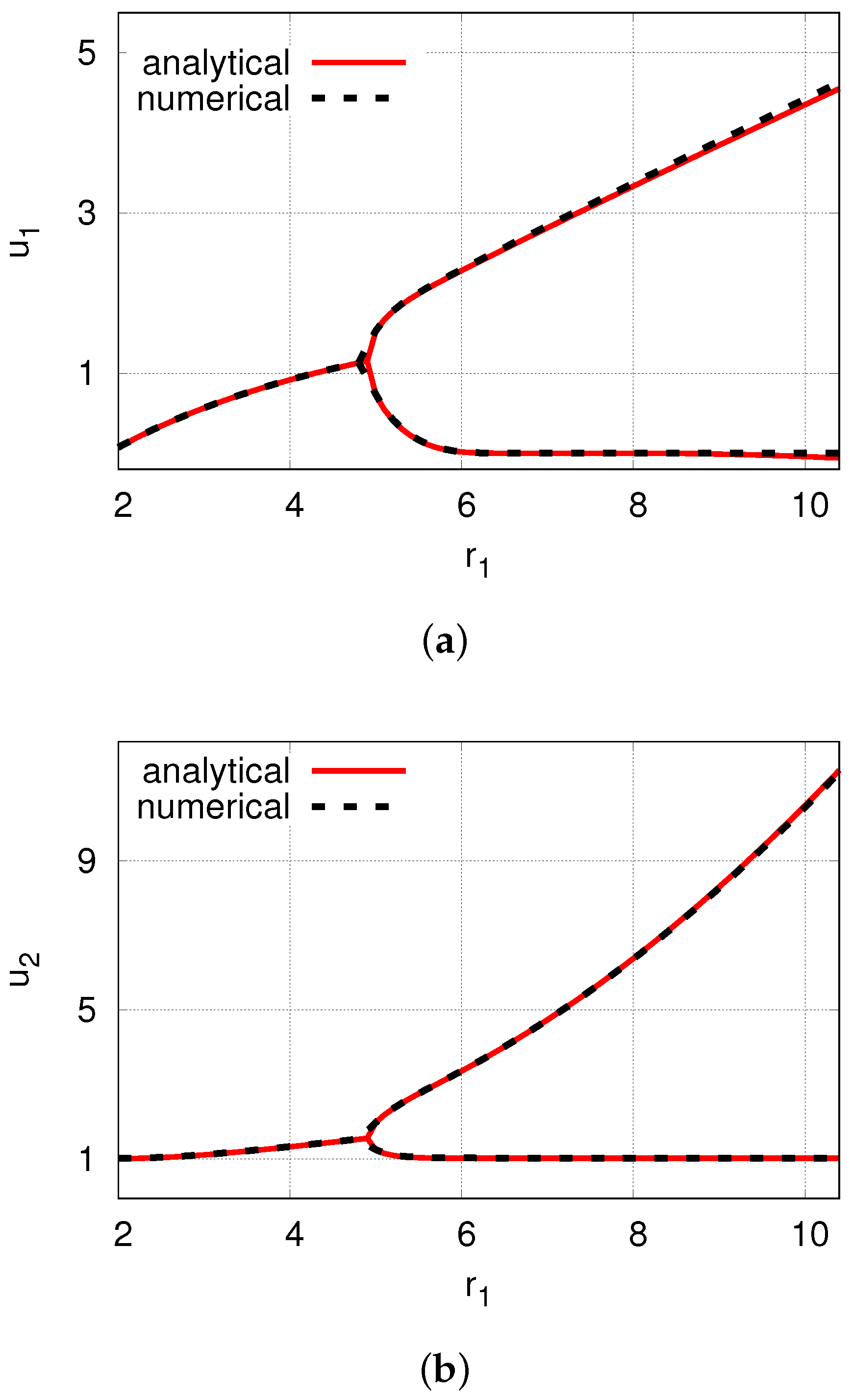
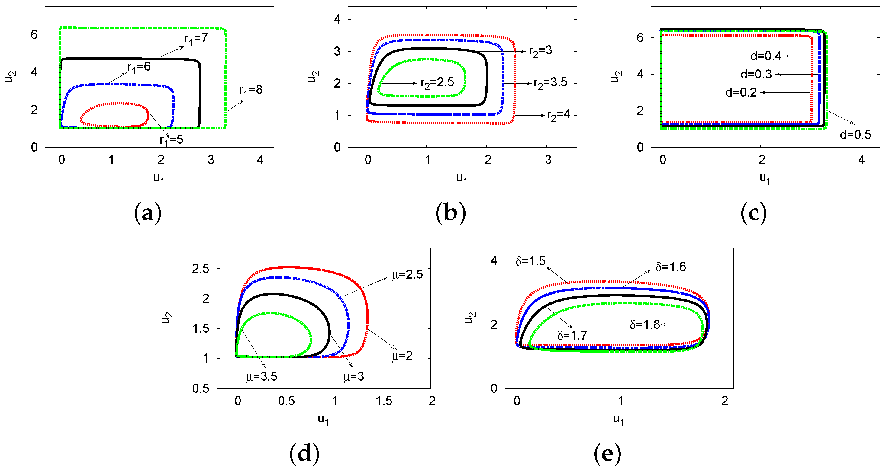
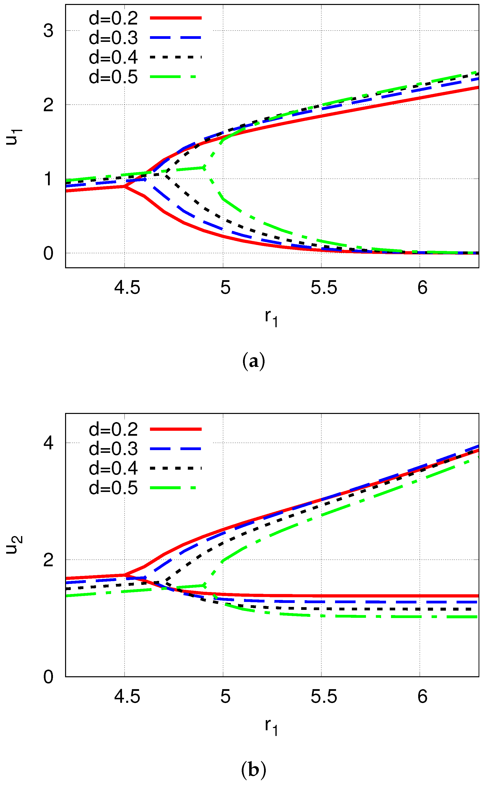
4.1. Bifurcation Diagrams and Periodic Solutions

Figure 14a,b show bifurcation diagrams for the two enterprise growth rates $u_1$ and $u_2$ versus the growth rate $r_1$. The analytical (red solid) and the numerical (black dots) outcomes are provided in both cases. These diagrams reveal the significant effect of incorporating delays into the model, which can induce instability. Steady-state solutions were found for the output of enterprise $u_1$ for growth rates $1.77\lesssim r_1<r_{1_{\mathrm{Hopf}}}$, and for $u_2$ between $\simeq 1.03<r_1<r_{1_{\mathrm{Hopf}}}$. After this supercritical Hopf bifurcation point, limit cycle results appear; the Hopf point is at $r_1\simeq 4.97$ (numerical PDE solutions) and $r_1\simeq 4.99$ (analytical ODE solutions). It can be seen from both plots that, as $r_1$ increases beyond $r_{1_{\mathrm{Hopf}}}$, and as the growth rate increases, the maximum oscillation amplitude grows, while the minimum amplitude decreases. The two-term theoretical solutions are consistent with the numerical PDE outcomes. The corresponding bifurcation map for the second growth rate $r_2$ exhibits a qualitatively similar behavior to that shown in this figure.

Figure 15a shows the evolution of the outputs of the two enterprises $u_1$ and $u_2$ at $x=0$ time t at a growth rate $r_1=4.5$, and Figure 1c,d show the steady-state spatial profiles $u_1$ and $u_2$ for $r_1=8$, which display a single central peak, (b) shows a 2-D phase-plane $u_1$–$u_2$ map. The solution in this example is stable in both figures (see the stable region in Figure 1c,d, showing the steady-state spatial profiles $u_1$ and $u_2$ for $r_1=8$, which display a single central peak). This figure corresponds to the regime when $r_1=4.5<r_{1_{\mathrm{Hopf}}}=4.97$ and the steady-state solution is formed at $u_1(0,t)=1.01$, and $u_2(0,t)=1.41$ when the time t is large enough. There is close agreement between the analytical ODE and numerical PDE results, within $1\%$ at time $t=42$. Figure 16a,b show results for a higher growth rate in the oscillatory region with $r_{1_{\mathrm{Hopf}}}=4.97<r_1=6$. The oscillation limit cycle appears and continues, with amplitudes $(u_1,u_2)=(2.28,3.36)$ for the ODEs and $(u_1,u_2)=(2.29,3.37)$ for the PDEs. The cycle period is $6.09$ for the analytic ODEs and $6.06$ for the numerical PDEs. The two methods agree to within $0.5\%$.

Figure 17 displays 2-D phase plots for the two enterprise outputs $u_1$ and $u_2$, showing the two-term ODE results for four cases of the parameters $r_1$, $r_2$, d, $\mu$, and $\delta$. Figure 17a–c show typical 2-D periodic orbits; it can be seen that, as the diffusion factor d and growth rates $r_1$ and $r_2$ were increased, the oscillation amplitudes grew moderately fast. In contrast, the oscillation limit cycle amplitudes decreased steadily with increased values of the rates $\mu$ and $\delta$, as can be seen in Figure 17d,e. Over time, it is apparent from Figure 1c,d, showing the steady-state spatial profiles $u_1$ and $u_2$ for $r_1=8$, which display a single central peak (d) and (e), that the oscillation disappeared and the stable region was entered when $\mu$ or $\delta$ was increased. These plots expand and confirm the solutions displayed in Figure 1c,d, showing the steady-state spatial profiles $u_1$ and $u_2$ for $r_1=8$, which display a single central peak and Figure 1c,d, showing the steady-state spatial profiles $u_1$ and $u_2$ for $r_1=8$, which display a single central peak.

Figure 18a,b show bifurcation diagrams for the two enterprise outputs $u_1$ and $u_2$, and the growth rate $r_1$, employing the analytic outputs with rates: $d=0.2$ (red dots), $0.3$ (blue dashes), $0.4$ (black solid), and $0.5$ (green dots). The supercritical Hopf points for both enterprises $u_1$ and $u_2$ are at $r_{1_{\mathrm{Hopf}}}\simeq 4.52$, $4.60$, $4.72$, and $4.91$ for diffusion parameters $d=0.2$, $0.3$, $0.4$, and $0.5$, respectively. It can be seen that decreasing the diffusion rate stabilized the system, whereas increasing d moved the enterprises $u_1$ and $u_2$ forward. However, the impact of the diffusion coefficient d on the growth rate $r_2$ was in the opposite direction: as the diffusion rate d increased, the Hopf-point values for the growth rate $r_2$ reduced, and the lines shifted back. These solutions confirmed the previous results shown in Figure 6a,b.

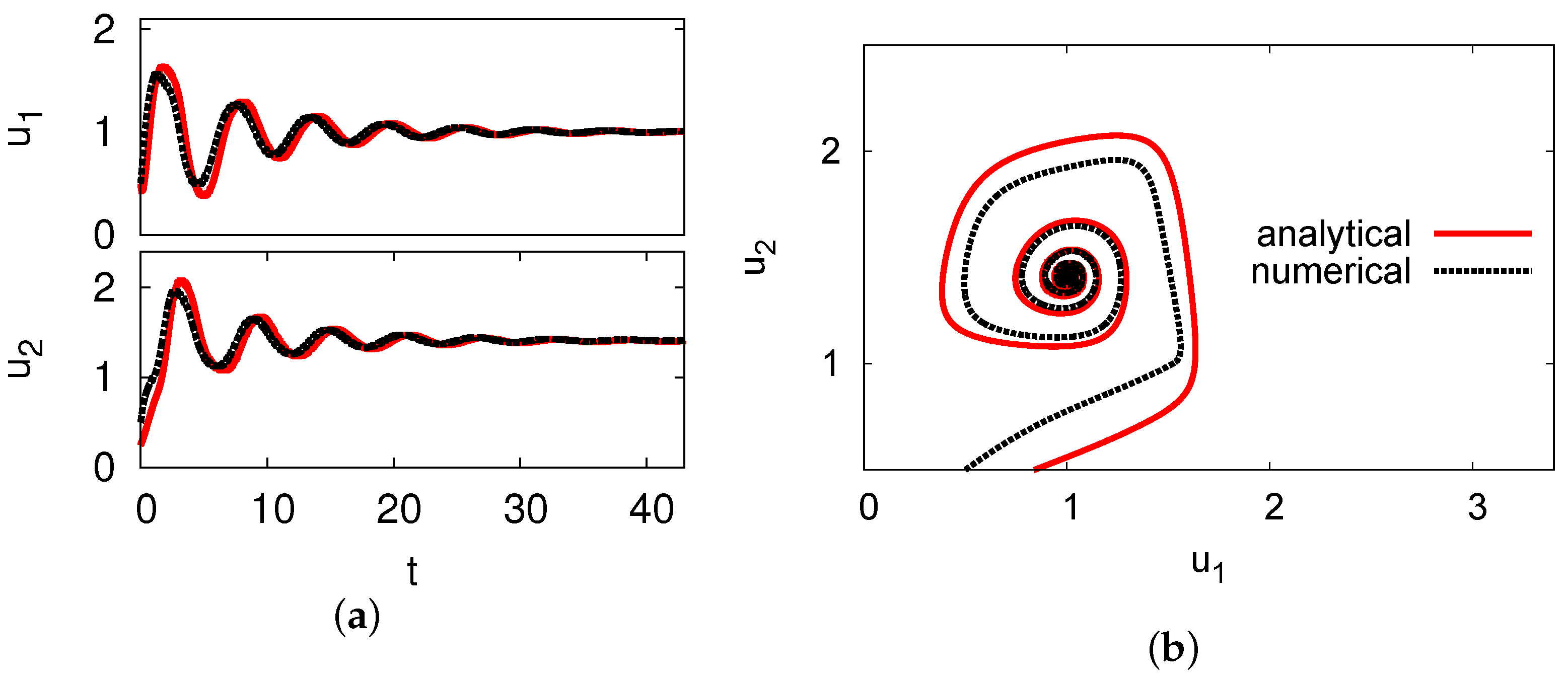
4.2. Numerical Simulation Examples

The exact location of the Hopf point for the growth rate $r_1$ and frequency $\omega$ is determined in this subsection, with various values of the time delay of output for the two enterprises, as $\tau =1,10,20,50,100,200$, as provided in

Table 1. Comparison between the analytical delay ODE (A1) results and numerical simulations of the delay PDEs (3) for varying growth rates $r_1$ and frequencies $\omega$.

		Growth rate (${\mathit{r}}_1$)			Frequency ($\mathit{\omega }$)
Case	Theoretical	Numerical	Error (%)	Theoretical	Numerical	Error (%)
$\tau =1$	5.491	5.578	≃1.56	1.116	1.159	≃3.71
$\tau =10$	5.447	5.455	≃0.15	1.056	1.072	≃1.49
$\tau =20$	5.407	5.411	≃0.07	0.999	1.006	≃0.60
$\tau =50$	5.394	5.397	≃0.06	0.981	0.985	≃0.40
$\tau =100$	5.387	5.389	≃0.04	0.971	0.974	≃0.30
$\tau =200$	5.383	5.384	≃0.02	0.966	0.968	≃0.21

. The other parameter values are ${\delta }_i=2$, $d_i=0.5$, ${\mu }_i=1$, $r_2=4$, and $c_i=0.1$. The table displays that, as $\tau$ grows, the disparity between the analytical ODE and numerical PDE solutions for the Hopf point $r_{1_{\mathrm{Hopf}}}$ and frequency $\omega$ decreases slowly, with the greatest discrepancy at ≃4%. The analytical solutions displayed in this table confirm the numerical outcomes plotted in Figure 1c,d, showing the steady-state spatial profiles $u_1$ and $u_2$ for $r_1=8$, which display a single central peak (a), and Figure 1c,d show the steady-state spatial profiles $u_1$ and $u_2$ for $r_1=8$, which display a single central peak. The approach taken by this study is validated by the excellent agreement between the theoretical outputs of the delay ODE and the numerical delay PDE results for all values of the growth rate $r_1$ and frequency $\omega$. For various systems, such as Nicholson’s blowflies [5], the delayed immune response [43,44], and the Schnakenberg model [34,42], period-doubling and chaotic outputs are observed for long time delays. However, in this example, these behaviors did not occur in either the PDEs or ODEs.

5. Conclusions, Economic Implications, and Outlook

This study focused on the effects of diffusion and delay in an economic system that modeled the interaction of outputs of two different enterprises in the same financial environment. The stability and Hopf bifurcations of a two-enterprise system with delays in a 1-D domain were investigated. The Galerkin technique was used to model the system of ODEs. The steady-state results and Hopf regions were examined both theoretically and numerically. Time delays and diffusion parameters were chosen as a bifurcation control to characterize the system’s stability behavior and to study the influences of these and other free parameters on the system. It was found that there were two different stability regions when ${\tau }_1,{\tau }_2>0$ (stable and unstable areas), and only one region when both time delays were zero, in which case, there was no Hopf point to explore and all outputs were stable. The Hopf-point value of the time delay increased with the diffusion rate. Moreover, when the delay time increased, the growth rates also increased, and the unstable region grew. Thus, the delay and diffusion parameters, with all other free parameters fixed, had a significant influence on the stability regions, with important economic implications. In addition, full diagrams were constructed for the three different cases of delays, showing their relationships with the other free parameters in this model. Bifurcation maps and 2-D charts were constructed to demonstrate, through various examples, the dependencies of periodic orbits. The main outcomes were confirmed through numerical simulations, indicating that the system exhibited a Hopf bifurcation, and several maps were plotted at large time values.

In conclusion, this study highlighted the significant role of the length of time delays for enterprises. Therefore, appropriate economic measures should be taken to ensure the stability of enterprise production. Further, enterprises can lose their stability and display periodic fluctuations, which means that overly long production cycles may lead to capacity fluctuations; diffusion may affect the amplitude of these fluctuations, which may be beneficial to the enterprises. Moreover, it can be shown that differences in the initial resources, the intrinsic growth rates, the time delays among different enterprises, or the position of an enterprise can have a substantial influence on its future development. In general, the results presented here illustrate the advantages of employing the Galerkin methodology, which yields a remarkable agreement with the PDE model with delays. In future research, we are planning to study the same model and methodology, augmented with four different delays, as presented in [18], and also to add a feedback term with delays, as in [21,27,31]. This study will including an exploration of state-state solutions, bifurcation, stability analysis, the Lindstedt–Poincaré perturbation method, and chaotic behavior, and may also apply them to a specific economic case study.

References

1. Alfifi, H.Y. Stability and Hopf bifurcation analysis for the diffusive delay logistic population model with spatially heterogeneous environment. Appl. Math. Comput. 2021, 408, 126362. [Google Scholar]
2. Alfifi, H.Y. Semi analytical solutions for the diffusive logistic equation with mixed instantaneous and delayed density dependencel. Adv. Differ. Equ. 2020, 2020, 162. [Google Scholar]
3. Feng, W.; Lu, X. On diffusive population models with toxicants and time delays. J. Math. Anal. Appl. 1999, 233, 374–386. [Google Scholar]
4. Noufaey, K.S.A.; Marchant, T.R.; Edwards, M.P. The diffusive Lotka-Volterra predator-prey system with delay. Math. Biosci. 2015, 270, 30–40. [Google Scholar] [CrossRef]
5. Alfifi, H.Y.; Marchant, T.R.; Nelson, M.I. Semi-analytical solutions for the 1- and 2-D diffusive Nicholson’s blowflies equation. IMA J. Appl. Math. 2014, 79, 175–199. [Google Scholar]
6. Taylor, M.P.; Kobiler, O.; Enquist, L.W. Alphaherpesvirus axon-to-cell spread involves limited virion transmission. Proc. Natl. Acad. Sci. USA 2012, 109, 17046–17051. [Google Scholar]
7. Alfifi, H.Y. Effects of diffusion and delayed immune response on dynamic behavior in a viral model. Appl. Math. Comput. 2023, 441, 127714. [Google Scholar]
8. Gu, Y.; Ullah, S.; Khan, M.A.; Alshahrani, M.Y.; Abohassan, M.; Riaz, M.B. Mathematical modeling and stability analysis of the COVID-19 with quarantine and isolation. Results Phys. 2022, 34, 105284. [Google Scholar] [CrossRef] [PubMed]
9. Manna, K. A non-standard finite difference scheme for a diffusive HBV infection model with capsids and time delay. J. Differ. Equ. Appl. 2017, 23, 1901–1911. [Google Scholar]
10. Noufaey, K.S.A.; Marchant, T.R. Semi-analytical solutions for the reversible Selkov model with feedback delay. Appl. Math. Comput. 2014, 232, 49–59. [Google Scholar]
11. Marchant, T.R. Cubic autocatalytic reaction diffusion equations: Semi-analytical solutions. Proc. R. Soc. Lond. 2002, A458, 873–888. [Google Scholar]
12. Alfifi, H.Y. Semi-analytical solutions for the diffusive Kaldor-Kalecki business cycle model with a time delay for gross product and capital stock. Complexity 2021, 2021, 9998756. [Google Scholar]
13. Fang, Y.; Xu, H.; Perc, M.; Tan, Q. Dynamic evolution of economic networks under the influence of mergers and divestitures. Phys. A Stat. Mech. Its Appl. 2019, 524, 89–99. [Google Scholar]
14. Kalecki, M. A macrodynamic theory of business cycles. Econometrica 1935, 3, 327–344. [Google Scholar]
15. Liao, M.; Xu, C.; Tang, X. Dynamical behaviors for a competition and cooperation model of enterprises with two delays. Nonlinear Dyn. 2014, 75, 257–266. [Google Scholar]
16. Hua, H.; Gashi, B.; Zhang, M. Robust risk-sensitive control. Int. J. Robust Nonlinear Control. 2023, 33, 5484–5509. [Google Scholar]
17. Hu, W.; Dong, T.; Zhao, H. Dynamic analysis of a competition-cooperation enterprise cluster with core-satellite structure and time delay. Complexity 2021, 2021, 6644292. [Google Scholar]
18. Li, L.; Zhang, C.; Yan, X. Stability and Hopf bifurcation analysis for a two-enterprise interaction model with delays. Commun. Nonlinear Sci. Numer. Simul. 2015, 30, 70–83. [Google Scholar]
19. Liao, M.; Xu, C.; Tang, X. Stability and Hopf bifurcation for a competition and cooperation model of two enterprises with delay. Commun. Nonlinear Sci. Numer. Simul. 2014, 19, 3845–3856. [Google Scholar]
20. Feng, C.; Pogue, O. The existence of periodic solutions for a two-enterprise interaction model with delays. Asian Res. J. Math. 2022, 9, 108–115. [Google Scholar]
21. Lu, L.; Lian, Y.; Li, C. Dynamics for a discrete competition and cooperation model of two enterprises with multiple delays and feedback controls. Open Math. 2017, 15, 218–232. [Google Scholar] [CrossRef]
22. Zhang, Y.; Li, L. Dynamic analysis on a diffusive two-enterprise interaction model with two delays. J. Math. 2022, 2022, 3466954. [Google Scholar] [CrossRef]
23. Xu, C. Periodic behavior of competition and corporation dynamical model of two enterprises on time scales. J. Quant. Econ. 2012, 29, 1–4. [Google Scholar]
24. Muhammadhaji, A.; Abdurahman, X. Dynamics in a competition and cooperation model of two enterprises with delays. Preprint, 2022. [Google Scholar] [CrossRef]
25. Szydłowski, M.; Krawiec, A. The Kaldor-Kalecki model of business cycle as a two-dimensional dynamical system. J. Nonlinear Math. Phys. 2001, 8 (Suppl. S1), 266–271. [Google Scholar] [CrossRef]
26. Guerrini, L. Small delays in a competition and cooperation model of enterprises. Appl. Math. Sci. 2016, 10, 2571–2574. [Google Scholar] [CrossRef]
27. Wang, Y. Permanence and stability for a competition and cooperation model of two enterprises with feedback controls on time scales. IAENG Int. J. Appl. Math. 2021, 51, 630–636. [Google Scholar]
28. Fletcher, C.A. Computational Galerkin Methods; Springer: New York, NY, USA, 1984. [Google Scholar]
29. Alfifi, H.Y.; Almuaddi, S.M. Stability analysis and hopf bifurcation for the Brusselator reaction—Diffusion system with gene expression time delay. Mathematics 2024, 12, 1170. [Google Scholar] [CrossRef]
30. Alfifi, H.Y. Semi-analytical solutions for the delayed diffusive food-limited model. In Proceedings of the 2017 7th International Conference on Modeling, Simulation, and Applied Optimization (ICMSAO), Sharjah, United Arab Emirates, 4–6 April 2017; pp. 1–5. [Google Scholar]
31. Alfifi, H.Y.; Marchant, T.R.; Nelson, M.I. Non-smooth feedback control for Belousov-Zhabotinskii reaction-diffusion equations: Semi-analytical solutions. J. Math. Chem. 2016, 57, 157–178. [Google Scholar] [CrossRef]
32. Alfifi, H.Y. Stability analysis and hopf bifurcation for two-species reaction-diffusion-advection competition systems with two time delays. Appl. Math. Comput. 2024, 474, 128684. [Google Scholar] [CrossRef]
33. Marchant, T.R.; Nelson, M.I. Semi-analytical solution for one-and two-dimensional pellet problems. Proc. R. Soc. Lond. 2004, A460, 2381–2394. [Google Scholar] [CrossRef]
34. Alfifi, H.Y. Stability analysis for schnakenberg reaction-diffusion model with gene expression time delay. Chaos Solitons Fractals 2022, 155, 111730. [Google Scholar]
35. Noufaey, K.S.A. Stability analysis for Selkov-Schnakenberg reaction-diffusion system. Open Math. 2021, 19, 46–62. [Google Scholar]
36. Erneux, T. Applied Delay Differential Equations; Springer: New York, NY, USA, 2009. [Google Scholar]
37. Hale, J. Theory of Functional Differential Equations; Springer: New York, NY, USA, 1977. [Google Scholar]
38. Looss, G.; Joseph, D.D. Elementary Stability and Bifurcation Theory, 2nd ed.; Springer: New York, NY, USA, 1990. [Google Scholar]
39. Smith, G.D. Numerical Solution of Partial Differential Equations: Finite Difference Methods, 3rd ed.; Oxford: New York, NY, USA, 1985. [Google Scholar]
40. Verwer, J.; Hundsdorfer, W.; Sommeijer, B. Convergence properties of the Runge-Kutta-Chebyshev method. Numer. Math. 1990, 57, 157–178. [Google Scholar]
41. Maplesoft, a Division of Waterloo Maple Inc. Maple; Maplesoft: Waterloo, ON, Canada, 2019. [Google Scholar]
42. Noufaey, K.S.A. Stability analysis of a diffusive three-species ecological system with time delays. Symmetry 2021, 13, 2217. [Google Scholar] [CrossRef]
43. Burić, N.; Mudrinic, M.; Vasović, N. Time delay in a basic model of the immune response. Chaos Solitons Fractals 2001, 12, 483–489. [Google Scholar] [CrossRef]
44. Canabarro, A.A.; Gléria, I.M.; Lyra, M.L. Periodic solutions and chaos in a non-linear model for the delayed cellular immune response. Phys. A Stat. Mech. Its Appl. 2004, 342, 234–241. [Google Scholar]
Figure 1. Steady-state densities for (a) u 1 and (b) u 2 against the growth rate r 1 , in the no-delay case τ = 0 , and steady-state spatial distributions of (c) u 1 and (d) u 2 with x for the case r 1 = 8 .
Mathematics 13 01026 g001
Figure 2. Steady-state solutions for the maps for (a) u 1 and (b) u 2 against r 2 , with τ = 0 , and steady-state spatial distributions for (c) u 1 and (d) u 2 for the special case r 2 = 10 .
Mathematics 13 01026 g002
Figure 3. (a,b) Bifurcation diagrams of the intrinsic growth rates r 1 and r 2 against the delay time τ .
Mathematics 13 01026 g003
Figure 4. Hopf bifurcation region in the d 1 τ map.
Mathematics 13 01026 g004
Figure 5. (a) Stability region of the d 1 d 2 plane for the case τ = 1 . (b) Hopf bifurcation regions for four cases τ { 1 , 2 , 3 , 4 } .
Mathematics 13 01026 g005
Figure 6. Bifurcation maps in the d 1 d 2 plane, with four different example rates r 1 ( a ) , r 2 (b), μ (c), and δ (d).
Mathematics 13 01026 g006
Figure 7. (a) Hopf bifurcation regions of the r 2 r 1 plane for the case τ = 1 . (b) Hopf bifurcation lines for four different values of the delay time τ .
Mathematics 13 01026 g007
Figure 8. Bifurcation curves of the of r 2 r 1 map, for different values of d (a), μ (b), and δ (c).
Mathematics 13 01026 g008
Figure 9. (a,b) Hopf bifurcation curves in the δ 2 δ 1 and μ 2 μ 1 maps.
Mathematics 13 01026 g009
Figure 10. Bifurcation maps of the r 2 r 1 plane (main plot) and the ω r 1 plane (inset). Two cases are considered: d i = 0 (no diffusion) and d i = 0.1 (with diffusion).
Mathematics 13 01026 g010
Figure 11. Bifurcation curves of growth rate r 1 versus τ 1 with different values of τ 2 .
Mathematics 13 01026 g011
Figure 12. Bifurcation maps in the r 2 τ 1 plane, with various values of τ 2 .
Mathematics 13 01026 g012
Figure 13. Hopf bifurcation curves in the d τ 1 (a), δ τ 1 (b), and μ τ 1 (c) planes, for various time delays τ 2 .
Mathematics 13 01026 g013
Figure 14. Bifurcation diagrams for the output of two enterprises, u 1 (a) and u 2 (b) against the growth rate r 1 .
Mathematics 13 01026 g014
Figure 15. (a) Time plot and (b) phase plot for the ODE and PDE systems, showing stable periodic orbits for the two enterprise outputs u 1 and u 2 at bifurcation parameter r 1 = 4.5 .
Mathematics 13 01026 g015
Figure 16. (a) Time plot and (b) phase plot showing a periodic solution for the numerical PDE and theoretical ODE systems beyond the Hopf bifurcation, which is orbitally unstable for both enterprise outputs u 1 and u 2 with r 1 =6.
Mathematics 13 01026 g016
Figure 17. Phase plots of system (A1) for two enterprises u 1 and u 2 with various values for r 1 (a), r 2 (b), d (c), μ (d), and δ (e).
Mathematics 13 01026 g017
Figure 18. Bifurcation diagrams for the u 1 r 1 (a) and u 1 r 2 (b) planes, for various rates of diffusion coefficients.
Mathematics 13 01026 g018