Abstract
This study presents an advanced second-order sliding-mode guidance law with a terminal impact angle constraint, which ingeniously combines reinforcement learning algorithms with the nonsingular terminal sliding-mode control (NTSM) theory. This hybrid approach effectively mitigates the inherent chattering issue commonly associated with sliding-mode control while maintaining high levels of control system precision. We introduce a parameter to the super-twisting algorithm and subsequently improve an intelligent parameter-adaptive algorithm grounded in the Twin-Delayed Deep Deterministic Policy Gradient (TD3) framework. During the guidance phase, a pre-trained reinforcement learning model is employed to directly map the missile’s state variables to the optimal adaptive parameters, thereby significantly enhancing the guidance performance. Additionally, a generalized super-twisting extended state observer (GSTESO) is introduced for estimating and compensating the lumped uncertainty within the missile guidance system. This method obviates the necessity for prior information about the target’s maneuvers, enabling the proposed guidance law to intercept maneuvering targets with unknown acceleration. The finite-time stability of the closed-loop guidance system is confirmed using the Lyapunov stability criterion. Simulations demonstrate that our proposed guidance law not only meets a wide range of impact angle constraints but also attains higher interception accuracy and faster convergence rate and better overall performance compared to traditional NTSM and the super-twisting NTSM (ST-NTSM) guidance laws, The interception accuracy is less than 0.1 m, and the impact angle error is less than 0.01°.
MSC:
93D05
1. Introduction
The traditional proportional navigation guidance (PNG) law is simple in form and easy to realize and has been widely used in engineering [1,2]. However, with modern warfare development, targets have become more and more defensive and maneuverable, necessitating missiles that not only achieve precise target strikes but also meet a specified terminal impact angle [3,4]. This is crucial for scenarios such as intercepting missiles with minimal impact angles for direct collision or striking vulnerable sections of targets like ground tanks and aircraft wings with optimal angles.
Current research into guidance laws with impact angle constraints primarily focuses on methods such as proportional navigation guidance’s additional bias term, optimal control theory, and sliding-mode variable structure control theory [5,6,7] among others. The basic idea of the proportional guidance method with an additional bias term [8,9,10] is to introduce an additional bias parameter to design a guidance law that meets the constraints of the miss distance and impact angle. The guidance law designed by this method is simple and easy to implement, but it mainly attacks stationary or slow-moving targets and lacks efficacy against rapid and highly maneuverable targets [11]. The optimal control method is also the most widely studied method; the idea is to find the guidance law with terminal impact angle constraint by minimizing the performance index. In [12], a guidance law with impact angle constraint that can hit maneuvering targets with constant acceleration is proposed based on the linear quadratic optimization theory. Reference [13] proposes a modeling method with the desired line of sight as the control target and designs an optimal guidance law for ballistic forming on the basis of constraining the relative motion direction of the terminal projectile and ballistic overload. The above optimal control methods achieve satisfactory control accuracy, but all of them require an estimation of the time-to-go, which can be challenging to ascertain in real-world scenarios.
Sliding-mode variable structure control has the characteristics of high precision and strong robustness, so it is widely used in the design of guidance laws with constraints [14,15]. In [16,17,18], the authors use a terminal sliding-mode (TSM) control method to design the guidance law, which can guarantee that the impact angle converges to the expected impact angle and the line-of-sight (LOS) angle rate converges to zero in finite time, and they apply the finite-time control theory to solve the specific convergence time. However, the existing TSM and fast terminal sliding-mode (FTSM) controllers have a common shortcoming, that is, the singular problem occurs easily on the terminal sliding-mode surface when the error approaches zero. To solve this problem, NTSM was proposed. NTSM can not only achieve finite time convergence but also avoid singularity problems; references [19,20,21,22] verify the above theory. It should be pointed out that in [20,22], in order to eliminate chattering, a special function is used to replace the sign function, which introduces steady-state errors, and the guidance laws above are all for non-maneuvering targets. For maneuvering targets, the authors of [23] achieve impact angle convergence by selecting the missile’s lateral acceleration to enforce the terminal sliding mode on a switching surface designed using nonlinear engagement dynamics, but they do not take into account the singularity that the proposed design may exhibit in its implementation. A guidance law based on NTSM is proposed in [19], but the maneuvering upper limit of targets needs to be estimated, and there are chattering problems. In order to suppress high-frequency chattering, the boundary-layer method, reaching law method, and observer method are all effective solutions. The authors in [24] used continuous saturation function to approximate the sign function, which reduced the chattering, but this method led to a decrease in the robustness of the system as the boundary layer increased. To solve this problem, reference [25] designed a second-order sliding-mode guidance law with continuous characteristics based on the high-order sliding-mode algorithm. The super-twisting algorithm was adopted as the reaching law of the sliding-mode control to eliminate the discontinuous term in the guidance law and thus weaken the chattering. However, the traditional super-twisting algorithm has the shortcomings of a slow convergence speed when the system state is far from the equilibrium point and cannot make full use of the missile overload capacity [26]. Nowadays, with powerful nonlinear approximation and data representation methods, data-driven reinforcement learning(RL) methods have attracted considerable attention in the design of guidance law, and model-free RL has been implemented in several algorithms for finding optimal solutions, making complex decisions, and in self-learning systems which improve behavior based on previous experiences [27]. Traditional reinforcement learning methods are suited for discrete environments with small action and sample spaces. However, real-world tasks, such as guidance and control challenges, involve large state spaces and continuous action domains with complex, nonlinear dynamics, which conventional methods find difficult to manage. Deep reinforcement learning (DRL) addresses these limitations by integrating deep neural networks with reinforcement learning, thereby enabling a more robust approach to handling the complexities of continuous and nonlinear systems. In recent years, many authors [28,29,30,31,32] have used Q-learning, deep Q-leaning network (DQN), deep deterministic policy gradient (DDPG), twin-delayed deep deterministic policy gradient (TD3), and other RL algorithms to train neural network models. The parameters of the missile’s LOS rate, position vector, and so on are used as state variables in a Markov decision as inputs, then the trained neural network can directly map the guidance command, which provides a new idea for the design of guidance law under multi-constraint conditions. Gaudet et al. [33] improved the Proximal Policy Optimization (PPO) algorithm and proposed a three-dimensional guidance law design framework based on DRL for interceptors trained with the PPO algorithm. A comparative analysis showed that the deduced guidance law also had better performance and efficiency than the extended Zero-Effort-Miss (ZEM) policy. In a similar way, Gaudet et al. [34] developed a new adaptive guidance system using reinforcement meta-learning with a recursive strategy and a value function approximator to complete the safe landing of an agent on an asteroid with unknown environmental dynamics. This is also a good method to solve the continuous control problem, but the PPO algorithm uses a random policy to explore and exploit rewards, and this method to estimate the accurate gradient requires a large number of random actions to find the accurate gradient. Therefore, such random operation reduces the algorithm’s convergence speed. In [35], an adaptive neuro-fuzzy inference sliding-mode control (ANFSMC) guidance law with impact angle constraint is proposed by combining the sliding-mode control method with an adaptive neuro-fuzzy inference system (ANFIS), and the ANFIS is introduced to adaptively update the additional control command and reduce the high-frequency chatter of the sliding-mode control (SMC), which enhances the robustness and reduces the chattering of the system; numerical simulations also verify the effectiveness of the proposed guidance law. In [36], the author proposes a three-dimensional (3D) intelligent impact-time control guidance (ITCG) law based on nonlinear relative motion relationship with the field of view (FOV) strictly constrained. By feeding back the FOV error, the modified time bias term including a guidance gain which can accelerate the convergence rate is incorporated into 3D-PNG; then, the guidance gain is obtained by DDPG in the RL framework, which makes the proposed guidance law achieve a smaller time error and have less energy loss. But in [37], the authors pointed out that the DDPG had the problem of an overestimation of the Q value, which may not give the optimal solution. Moreover, the DDPG uses a replay buffer to remove the correlations existing in the input experience (i.e., the experience replay mechanism) [38,39] and uses the target network method to stabilize the training process. As an essential part of the DDPG, experience replay significantly affects the performance and speed of the learning process by choosing the experience used to train the neural network.
Based on the above problems, this paper designs a novel adaptive impact angle-constrained guidance law based on DRL and the super-twisting algorithm. It introduces a parameter to replace the fractional power equal to one half in the conventional super-twisting algorithm, which improves the guidance performance and the convergence rate of the system state by adaptively adjusting this parameter. Drawing on the insights from [37,40], we apply the preferential sampling or prioritized experience replay mechanism [41] to enhance the TD3 algorithm and then obtain the adaptively optimal parameters using our improved DRL algorithm. Compared to the sliding-mode guidance law based on the traditional super-twisting algorithm, our algorithm is more effective in reducing chattering, has better guidance accuracy, and achieves better constraint effects on the terminal impact angle. Moreover, the trained neural network exhibits strong generalization capabilities in unfamiliar scenarios. Finally, we design a GSTESO, different from the modified ESO in [42] that only uses nonlinear terms; the proposed GSTESO can provide faster convergence rate when the estimation error is far away from the equilibrium, and it does not depend on an upper bound of uncertainty. Furthermore, in comparison to the modified ESOs incorporating both linear and nonlinear terms discussed in [43], the GSTESO we propose does not introduce any additional parameters that require adjustment.
2. Preliminaries and Problem Setup
2.1. Relative Kinematics and Guidance Problem
The missile–target relative motion relationship is established in the inertial coordinate system, as shown in Figure 1, where is the ground inertial coordinate system, r is the missile–target relative distance, q is the missile–target LOS angle, M and T are the interceptor and the target, and are the flight path angle of the missile and the target, respectively, V and represent the velocity of the missile and the target, respectively, and represent the normal acceleration of the missile and the target, respectively, and are the parameters of leading angles of the missile and the target. It is stipulated that all angles in Figure 1 are positive counterclockwise.
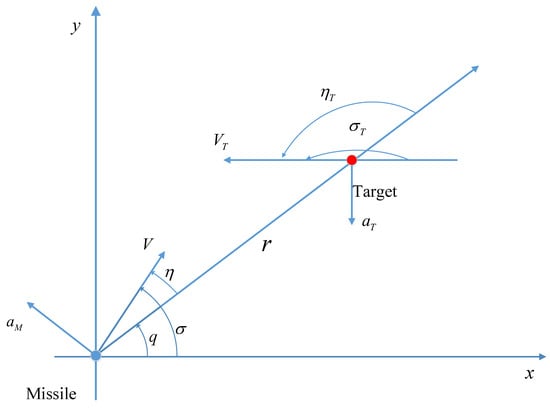
Figure 1.
Relative motion model ( is perpendicular to V, is perpendicular to ).
According to the missile–target relative motion relationship in Figure 1, the dynamic model of the missile terminal guidance phase is obtained as
where is the relative speed between the missile and the target; is the LOS rate. According to the constant-bearing course, a guidance law is designed to make the LOS angle rate converge in a finite time to ensure that the missile can accurately attack the target.
The impact angle is defined as the angle between the missile velocity vector and the target velocity vector at the interception of the guidance phase during the missile’s attack on the target. The moment when the missile intercepts the target is denoted as , and the desired impact angle of the missile in the guidance process is denoted as .
Lemma 1
([44]). For a pre-designated target with an expected impact angle, there always exists a unique desired terminal LOS angle. Hence, the control of the intercept angle can be transformed into the control of the final LOS angle.
Assuming that the desired LOS angle is , the objective of this paper translates into designing a continuous guidance law that achieves , in finite time.
2.2. Kinematic Equations for LOS Angle Tracking Error
We take the first derivative of Equation (1) and Equation (2), respectively, to obtain
where , is the acceleration of the missile and the target along the LOS angle, respectively, , ; , is the acceleration of the missile and the target normal to the LOS angle direction, respectively. For most tactical missiles controlled by aerodynamic forces, the axial acceleration along the velocity direction is often uncontrollable, so this paper only designs the guidance law based on Equation (6).
Let e be the LOS angle tracking error, and the LOS angle rate . Then, the LOS angle second-order dynamic error equation can be obtained as:
2.3. Deep Reinforcement Learning
The deep reinforcement learning algorithm is an algorithm based on the actor–critic network structure, which can update policy and value function at the same time and is suitable for solving decision problems in the continuous task space. Using the DDPG [45] algorithm as an example, the actor network uses policy functions to generate action , which is executed by agents to interact with the environment. The critic network uses the state-action value function to evaluate the performance of the action and instruct the actor network to choose a better action for the next stage.
The actor network uses a policy gradient algorithm to update parameter :
The actor network uses the estimated value obtained by the critic network to select actions, so the estimate should be as close to the target value as possible, which is defined by:
where represents the current reward, represents the next state, is the state-action estimate obtained by the critic target network, and is the estimated action obtained by the actor target network. All target networks use the “soft update” method to update network parameters.
The training of the critic network is based on minimizing the following loss function to update the new parameter w:
When the two networks obtain the optimal parameters, the whole algorithm can obtain the optimal strategy, which can be regarded as a mapping from state to action, so that the missile can select the most valuable action according to the current environment state.
3. Guidance Law Design with Impact Angle Constraint
3.1. Disturbance Differential Observer Design and Stability Analysis
The observer proposed in this paper is the GSTESO, whose role is to observe the disturbance in real time. Its input is the measurable system state parameters, and its output is the observed value of the disturbance, which is used for system compensation.
Consider the following system:
where z is the controlled variable, u is the control variable, and d is the disturbance.
Assuming that the upper limit of target acceleration is known [46], and due to the limitation of physical conditions, there is always an upper limit of . Therefore, assuming that is known, it is easy to know that the disturbance term also has an upper limit, that is:
Let system disturbance ; Equation (6) becomes
Let ; Equation (6) can be written as
According to Equations (12) and (15), the proposed GSTESO can be constructed as follows:
where , and the nonlinear function is designed as
where the symbol is defined as , and the parameter of GSTESO can be selected as , .
Similarly, let ; the estimation error system can be written as:
Next, we verify the stability of the GSTESO. Firstly, let us introduce a new state vector as follows
The Lyapunov function is constructed as
where P is a symmetric and positive definite matrix, and the derivative of is
where ,
Inspired by [43], we set , where ; then, it can be guaranteed that by choosing proper matrices C and D.
Theorem 1
([43]). Suppose there exists a positive definite symmetric matrix P and positive constant κ satisfying the following matrix inequality:
System (18) is finite-time stable.
According to Equation (20), we can obtain the final result as follows:
where is the eigenvalue of matrix P, and .
Therefore, holds, and Equation (24) can be rewritten as
According to the finite-time stability criterion mentioned in [47], the error system (18) achieves finite-time stability.
3.2. Guidance Law Design
The sliding-mode control can be divided into two phases: the first phase is the reaching period, during which the system state converges from the initial state to the sliding-mode surface under the action of the auxiliary control term. The second phase is the sliding phase, in which the system state slides along the sliding-mode surface to the equilibrium point under the action of the equivalent control term to achieve state convergence.
Terminal sliding-mode control uses a nonlinear function as a sliding surface, which can make the system state converge in finite time, but this method has a singularity problem. In order to avoid the singularity problem and obtain higher control accuracy and faster convergence speed [48], this paper uses the non-singular terminal sliding-mode surface to design the guidance law. The sliding surface is designed by:
where are design parameters, .
The super-twisting algorithm is a second-order sliding-mode algorithm, which has been widely used in control problems because of its superior characteristics such as effectively reducing the chattering, strong robustness, and high-precision control.
The adaptive super-twisting algorithm is as follows:
The algorithm converges in finite time. The proof can be found in reference [49,50].
According to Equations (27) and (28) and reference [51], the proposed RLST-NTSM is given by:
where are design parameters, is the introduced adaptive parameter, and is the output of the GSTESO Equation (16).
Remark 1.
While the traditional super-twisting method directly sets the parameter to 2, we introduced a free parameter γ in Equation (28). Various papers [26,52,53,54,55,56,57] have proposed different adaptive methods to improve the super-twisting sliding-mode guidance law, each with its own specific form. However, most of these methods involve an adaptive gain adjustment of the parameter . The study [50] already showed that for the traditional super-twisting algorithm, as long as was sufficiently large, the algorithm could converge. As for the impact of parameter variation involved in the equation on control effectiveness, there is currently no literature studying this aspect, with only a few references (e.g., [58]) mentioning choosing a value slightly greater than 0.5 for . This suggests that some researchers may have already found that directly selecting the value as may not be appropriate. Therefore, this paper employed DRL algorithms to adaptively adjust the selection of this parameter through model-free learning to achieve adaptive tuning.
3.3. Stability Analysis
Before delving into the analysis, let us introduce Lemma 2 [59]:
Lemma 2
([59]). Suppose , defined on , , is a smooth positive definite function, and is a negative semi-definite function on for and ; then, there exists an area such that any which starts from can reach in finite time , and the settling time can be estimated by
where is the initial value of .
Taking the derivative of Equation (27) with respect to time, we obtain
According to Section 3.1, the estimation error of the GSTESO in (16) is dynamically finite-time stable, when the observer observation error tends to 0, and Equation (32) can be simplified as follows
Referring to reference [49], we introduce a new state vector as follows
where , .
Since , it is easy to prove that A is a Hurwitz matrix. Thus, there exists a unique matrix and P is the solution of the following Lyapunov equation.
where every .
For the stability analysis of Equation (35), we choose the following Lyapunov function:
Taking the derivative of Equation (38) and substituting Equations (34) and (35), we obtain
From the definition of , we know that , where denotes the L2-norm of the vector; then, Equation (39) becomes
where and are the minimum eigenvalue and maximum eigenvalue of matrix , , . According to Lemma 3, when , the equilibrium point of the system in Equation (35) is finite-time stable, and the convergence time is satisfied
where denotes the value of V at time . It follows from the definition of that Equation (27) for the nonsingular terminal sliding-mode surface can also converge in finite time. Once the sliding-mode surface is reached, Equation (27) is obtained
In summary, the system in Equation (34) is finite-time stable.
3.4. Algorithm Design for Reinforcement Learning
Reinforcement learning considers the paradigm of interaction between an agent and its environment, and its goal is to make the agent take the behavior that maximizes the benefit, so as to obtain the optimal policy. Most reinforcement learning algorithms are based on a Markov decision process (MPD). The MPD model is often used to establish the corresponding mathematical model for a decision problem with uncertain state transition probability and state space and action space and to solve the reinforcement learning problem by solving the mathematical model. If the simulation covers all the state spaces encountered by the guidance law in practice and there is sufficient sampling density, the resulting guidance law is the optimal one with respect to the modeled missile and environment dynamics.
To better solve the problem in this paper, we chose the LOS angle rate, LOS angle tracking error, as well as the sliding-mode value as the state space , which can also cover the whole guidance process. Then, the neural network was used to map the state of each step out of the parameter in Equation (28). Through Equation (40), we know , so can be obtained; thus, we designed the action space as . Considering the overload problem in real flight, we restricted the action space to 200 m/s2.
The reward function acts as a feedback system to indicate from the environment whether the missile performance is good or bad. In order to further reduce the chattering problem and improve the guidance accuracy, the reward function designed in this work was divided into two parts.
We shaped the shaping reward function as follows:
where is the weight parameter, and the maximum values of and were set to 100 and 10,000, respectively.
In standard reinforcement learning, the aim is to maximize the long-term reward for the agent’s interaction with the environment. The goal of the agent is to learn a policy that maximizes the long-term reward: , where T is the termination time step, is the reward the agent would receive for performing action in state , and is the discount factor . The action value function is used to represent the expected long-term reward for performing action in state :
Using the Bellman equation to compute the optimal behavioral value function, the above equation becomes
The reinforcement learning algorithm used in this paper was based on the TD3 algorithm. Compared with the DDPG algorithm mentioned in Section II, this algorithm has three differences: (1) it uses two critic network modules to estimate the Q value, (2) it has delayed policy updates, and (3) it uses target policy smoothing.
The first is also known as Clipped Double-Q learning. TD3 has two critic networks and two critic target networks. Both target networks produce a value and use the smaller one as the new target.
where , are the Q values generated by the two critic target networks, respectively, and represents the next state. When updating the policy, because the actor network module selects the maximum Q value in the current state, Equation (48) can effectively reduce the overestimation error. Then, we take the above equation and calculate the mean squared error (MSE) of the values generated by the two critic networks, and we can obtain the loss function of the critic network.
where stands for the parameters of the two critic networks, D stands for the replay buffer, and are the Q values produced by the two critic models, respectively.
The next point is the target policy smoothing; if the D estimate produces an incorrect peak, the policy network is immediately affected, and then the performance of the whole algorithm is affected, so clipping noise was added to the target policy generation operation. Then, the action was clipped within the valid range, and Equation (48) was formulated as follows:
where is the policy generated by the actor network, is the clipping noise, and and refer to the upper and lower bounds of the action space, respectively. Adding noise at the target value is equivalent to adding a regularization term to the critic. In the process of sampling multiple times, obtains slightly different values according to different sampling noise, and y evaluates the average of the value functions of these sampling points. Therefore, y reflects the overall situation of the value functions around . This way, it is not affected by some extreme value functions, and the stability of critic learning is enhanced.
The last point is to delay policy update. DDPG and TD3 both focus on how to learn a good critic, because the more accurate the critic estimates, the better the policy obtained by actor training. Therefore, if the critic is poorly learned and its output has large errors, the actor is also affected by preorder errors in the learning process. TD3 proposes that the critic should be updated more frequently than the actor, that is, the policy should be updated after getting an accurate estimate of the value function, and in this paper, the value function was updated five times before the policy function was updated.
3.5. Prioritized Experience Replay
The core concept of prioritized experience replay is to replay more frequently experiences associated with very successful attempts or extremely poor performance. Therefore, the key issue lies in defining the criteria for determining experience value. In most reinforcement learning algorithms, the TD error is commonly used to update the estimation of the action value function . The magnitude of the TD error acts as a correction for the estimation and implicitly reflects the agent’s ability to learn from experiences. A larger absolute TD error implies a more significant correction to the expected action value. Furthermore, experiences with high TD errors are more likely to possess a high value and be associated with highly successful attempts. Similarly, experiences with large negative TD errors represent situations where the agent performs poorly, and these conditions are learned by the agent. Prioritized experience replay helps gradually realize the actual consequences of incorrect behavior in corresponding states and prevents repeating those mistakes under similar circumstances, thereby enhancing overall performance, so these unfavorable experiences are also considered valuable. In this paper, we adopted the absolute TD error as an index for evaluating experience value. The TD error of experience j can be calculated as:
where y is obtained from Equation (49), and is the Q value generated by the two critic models, respectively.
We defined the probability of sampling experience j as
where , , represents the priority of experience j in replay buffer, and the parameter is used to adjust the priority level. The definition of sampling probability can be regarded as a method to add a random factor when selecting experiences, because even experiences with a low TD error can still have the probability of replay, which ensures the diversity of sampling experiences. This diversity helps to prevent any overfitting of the neural network.
Because our priority experience replay changed the sampling method, the importance sampling weight was used to correct the error introduced by the priority replay, and the loss function of the network for gradient training was calculated to reduce the error rate of the model. The importance sampling weights were calculated as follows:
where is the adjustment factor of .
Based on the several algorithms introduced above, an adaptive integrated guidance algorithm with impact angle constraint based on deep reinforcement learning is presented in the following Figure 2.
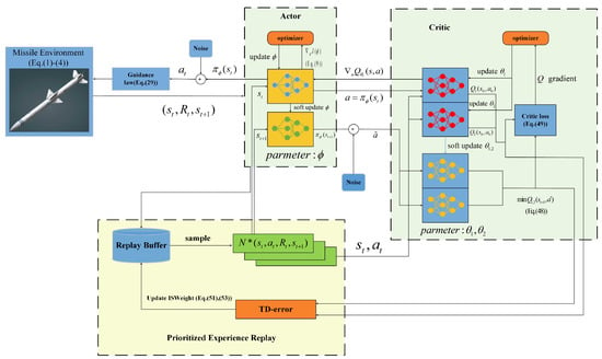
Figure 2.
Schematic of the PERTD3-based RL guidance law ( represents the adaptive parameter to be output at time t, represents the , captured by the seeker at time t, in addition to the step of environmental interaction, which includes the update of parameters such as position, angle, sliding variable, etc., the rest of the equation number is one step, and each step can be found in the pseudo-code).
The TD3 algorithm with prioritized experience replay (PERTD3) is shown in Algorithm 1.
| Algorithm 1 Guidance law’s learning algorithm based on the PERTD3 algorithm |
|
4. Simulation and Analysis
In this section, we considered two maneuver modes, a sinusoidal maneuver and a constant maneuver, and then tested them from three aspects: flight trajectory, normal acceleration, and LOS angle rate. Finally, the performance of the three guidance laws was analyzed in terms of miss distance.
First, when the target was on a sinusoidal maneuver, the PERTD3 and TD3 algorithms were both trained 10,000 times using the parameters in Table 1 and Table 2. Both actor network and critic network were implemented by a three-layer fully connected neural network, Critic1 and Critic2 used the same network structure; the network structure is shown in Figure 3. Except for the output layer of critic, the neurons in all other layers were activated by a ReLu function, i.e.,

Table 1.
Dynamic model’s initial simulation parameters.

Table 2.
Hyperparameters for TD3 algorithm [32].
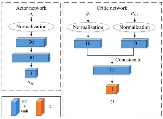
Figure 3.
The network structure of PERTD3.
The output layer of the critic network was activated by the tanh function, which is defined as
The policy and value functions were periodically updated during optimization after accumulating trajectory rollouts of the replay buffer size.
As shown in Figure 4, our improved deep reinforcement learning algorithm was better than two other existing deep reinforcement learning algorithms in our written dynamic environment. The guidance algorithm based on PERTD3 and TD3 basically converged when approaching 800 steps, but the TD3 algorithm with prioritized experience replay could achieve higher scores and had higher stability, while the DDPG algorithm did not converge at the end.
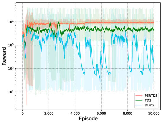
Figure 4.
Comparison of learning curves of the three algorithms.
To verify the robustness of our algorithm, we took the following two maneuvers and the case of the required impact angle constraint, and case 1 was not used during training but was used to test the generalization of our reinforcement learning algorithms.
Case 1: The target performed a constant maneuver , i.e., the impact angle constraint was for every .
Case 2: The target performed a constant maneuver , i.e., the impact angle constraint was for every .
As shown in Figure 5 and Figure 6, the simulation results in case 1 are shown in Figure 5, and the simulation results in case 2 are shown in Figure 6. From Figure 5a,c,d and Figure 6a,c,d, Table 3 and Table 4, it can be seen that the missile could accurately hit the target with the desired terminal LOS angle in a limited time, the LOS angle rate converged to 0°/s, and the LOS angle converged to the expected value under different desired LOS angles, which verified the superstrong control ability of the guidance law for the miss distance and the impact angle. From Figure 5b and Figure 6b, it can be seen that the missile acceleration command was smooth. Since the control law was continuous with respect to the sliding variable, it can be seen that the sliding variable converged to zero continuously and smoothly in finite time in Figure 5e and Figure 6e, and the chattering phenomenon did not appear in the control channel. It can be seen from Figure 5f and Figure 6f that the disturbance differential observer could achieve a great estimation of the system uncertainty. As can be seen from the overall Figure 6, when facing untrained scenes, our improved reinforcement learning algorithm could still hit the target, and the LOS angle converged, which proves that our algorithm has generalization and practical significance.
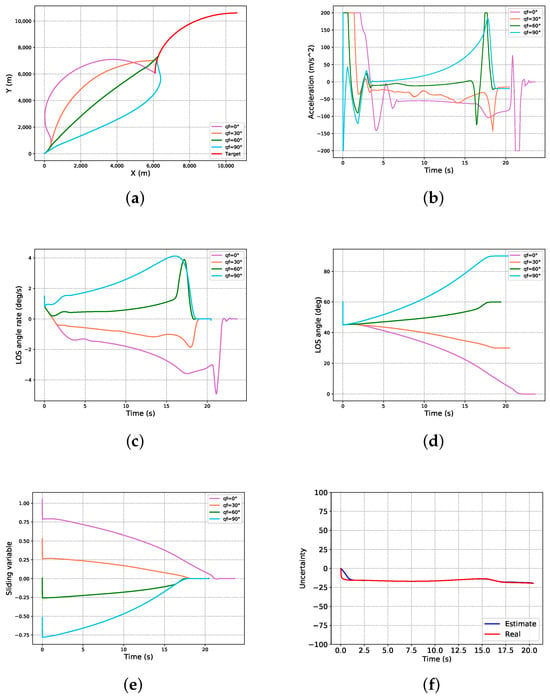
Figure 5.
Simulation results for case 1: (a) trajectories of missile and target; (b) missile acceleration commands; (c) LOS angle rate; (d) LOS angle; (e) sliding-variable profiles; (f) GSTESO estimation.
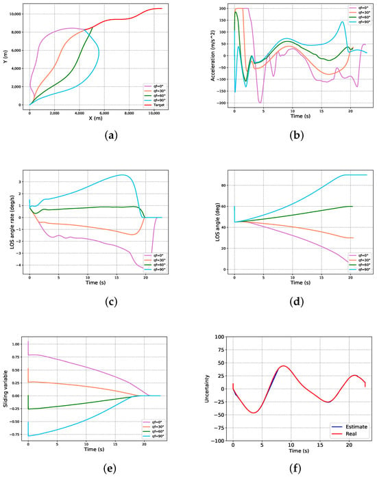
Figure 6.
Simulation results for case 2: (a) trajectories of missile and target; (b) missile acceleration commands; (c) LOS angle rate; (d) LOS angle; (e) sliding-variable profiles; (f) GSTESO estimation.

Table 3.
Statistics of guidance simulation results in case 1.

Table 4.
Statistics of guidance simulation results in case 2.
In Figure 7, Figure 7a is the parameter change for case 1, and Figure 7b is the parameter change for case 2. It can be seen from the figure that the parameter change finally converged to between two and three, and the change process was smooth, which is of practical engineering significance.
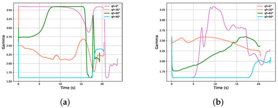
Figure 7.
The variation trend of parameter : (a) curve of parameter for case 1; (b) curve of parameter for case 2.
In order to show the advantages of our guidance law, we compared with ST-NSTM and NSTM guidance laws, and we set the miss distance to less than 0.1 m. Our algorithm could call the RLST-NTSM guidance law. The parameters of Equation (20) were borrowed from the literature [58], where , , and then we chose , , after the comparison. The in the ST-NTSM guidance law was the same as before, and the traditional super-twisting non-singular terminal sliding-mode guidance law (ST-NTSM [51]) was formulated as:
where is the output of the finite-time convergence disturbance observer (FTDO). According to the reference [58], the specific form of the FTDO [60] introduced by the author in his article is as follows:
where the choice of in the equation can be obtained from [58]. The parameter L is used to adjust the transient performance of the estimation process and can be set to 200, which makes the observer output converge to in finite time.
In addition, another extended state observer based on the traditional super-twisting extended state observer (STESO) [42] was also added for comparison; it was formulated as:
where , were the same as in the GSTESO.
And the NSTM guidance law was of the form:
where the values of were also the same as before, and the value of the switching gain K was 400 according to reference [58].
As shown in Table 5 and Figure 8, we simulated different values corresponding to ST-NTSM for case 2. It can be seen from Table 5 that no matter how the parameter value was selected, the accuracy of ST-NTSM was not as high as our algorithm, only the values of 2.3 and 2.6 qualified, given that the miss distance had to be less than 0.1 m. Figure 8 also shows that ST-NTSM still had a small number of chattering problems. And as the parameter increased, the convergence rate of the guidance law was slower, while our guidance law converged faster, and the chattering phenomenon did not occur.

Table 5.
Statistics of simulation results for case 2 with different parameter values.
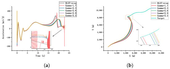
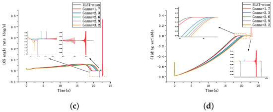
Figure 8.
Comparison of guidance laws with different parameters for case 2: (a) missile acceleration commands; (b) trajectories of missile and target; (c) LOS angular rate; (d) sliding-variable profiles.
The simulation results for case 2 with are shown in Figure 9 and Table 6. The RLST-NTSM proposed in this paper was better than the other two guidance laws in terms of accuracy and convergence of the final LOS angle error, and Figure 9b shows that the missile guided by NTSM did not hit the target, while the performance of ST-NTSM was relatively good. However, according to Figure 9a,d, there was still a certain chattering phenomenon, and the proposed algorithm further reduced the system chattering. It can also be seen from Figure 9c that RLST-NTSM reached the equilibrium state of the system earlier than ST-NTSM. From Figure 9d,e, it can be seen that the sliding-mode variable and LOS angle rate of ST-NTSM and NTSM did not converge well, which would greatly affect their practical engineering application. Finally, it should be noted that although the three observers could be directly added to any guidance law, it can be seen from Figure 9f–h that the GSTESO performed better than the other two observers, as its initial uncertainty observation error was minimal.
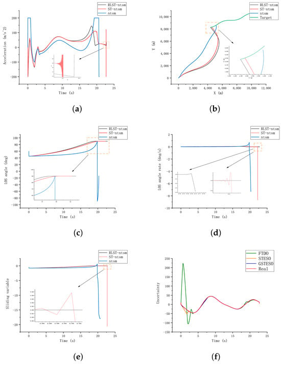
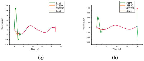
Figure 9.
Comparison for three guidance law and three observer under case 2: (a) missile acceleration commands; (b) trajectories of missile and target; (c) LOS angle; (d) LOS angular rate; (e) sliding-variable profiles; (f) three observers’ estimation in RLST-NTSM. (g) three observers’ estimation in ST-NTSM; (h) three observers’ estimation in NTSM.

Table 6.
Statistics of simulation results for case 2 with different parameter values.
As overload saturation emerged in the simulation, we eventually decided to consider the constraints of the autopilot in a simplified manner; combined with Equation (14), we studied the following augmented system.
where , is the modeling error, and are the damping ratio and natural frequency of the autopilot.
This paper employed an autopilot approach similar to the one described in reference [61], and its formulation is given by
where , .
We selected the virtual control signal as in Equation (29). The first and second derivatives of were estimated using the following filter instructions:
where , and are the damping ratio and natural frequency of the command filter, respectively, and are the estimate and the corresponding derivative, respectively, and are positive constants. The system was observed using the following ESO
where are the estimate errors, , and are the positive observer gains to be designed, , and is a small positive constant.
The stability of the autopilot component can be established by consulting reference [61], and a detailed analysis was not conducted. The autopilot parameters were . The design parameters for implementing guidance law (61) were set to and . The parameters of the ESOs were selected as .
As illustrated in Figure 10 and Table 7, this paper focused on simulating the scenario that produced the maximum normal overload, specifically, in case 2; the results showed that considering the autopilot lag characteristics did not affect the performance of the proposed guidance law.
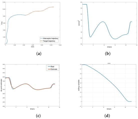
Figure 10.
Simulation results considering the autopilot lag: (a) trajectories of missile and target; (b) missile acceleration commands; (c) autopilot error estimate; (d) LOS angular rate.

Table 7.
Simulation results considering the autopilot lag for case 2.
5. Conclusions
In this study, we proposed a novel guidance law, named RLST-NTSM, which combined deep reinforcement learning with sliding-mode guidance. That guidance law was specifically designed for the interception of maneuvering targets with terminal LOS angle constraints. The RLST-NTSM guidance law enhanced the traditional ST-NTSM by introducing an adaptive gamma parameter, which was optimized through a DRL algorithm to achieve optimal adaptive control. Through the design of the reward function, it effectively reduced the chattering phenomenon and improved the convergence rate of the system state; this is beneficial to improve the stability of the missile body during the actual flight. Furthermore, a GSTESO was employed to estimate and compensate for system disturbances. Distinguished from conventional STESO and FTDO, the GSTESO provided stronger robustness and disturbance rejection ability. Utilizing Lyapunov’s stability theory, we proved the finite-time convergence of the closed-loop guidance system. Simulation results showed that our algorithm greatly improved the overall performance compared with the traditional ST-NTSM and NTSM, and the interception accuracy was improved by at least five times. In response to the emergence of overload saturation within our simulations, we considered the delay characteristics of the autopilot in the concluding segment of our study. Our analysis revealed that these constraints did not impair the guidance performance. In the future, the primary objective of the subsequent phase of research will be to expand the guidance environment into a three-dimensional space. Following this, we intend to deploy the guidance algorithm in a real-world setting to conduct experimental trials.
Author Contributions
Conceptualization, Z.H. and W.Y.; methodology, Z.H.; investigation, Z.H.; writing—original draft preparation, L.X.; writing—review and editing, L.X.; funding acquisition, W.Y. and L.X. All authors have read and agreed to the published version of the manuscript.
Funding
This work has been supported by the National Natural Science Foundation of China (Grant No. 62471235).
Data Availability Statement
The original contributions presented in this study are included in the article. Further inquiries can be directed to the corresponding author.
Conflicts of Interest
The authors declare no conflict of interest.
Nomenclature
| MDP | Markov Decision Process |
| RL | Reinforcement learning |
| s | State vector in the MDP |
| a | Action vector in the MDP |
| The parameter of the critic network | |
| The parameter of the actor network | |
| Reward for being in states when selecting the corresponding action a at time t | |
| The cumulative sum of subsequent rewards after time point t | |
| The probability density p associated with random variable x | |
| Expectation of , i.e., | |
| The action value for an agent taking action a by following policy in the state at time t |
References
- Ristic, B.; Beard, M.; Fantacci, C. An overview of particle methods for random finite set models. Inf. Fusion 2016, 31, 110–126. [Google Scholar] [CrossRef]
- Liu, D.; Wang, Z.; Liu, Y.; Alsaadi, F.E. Extended Kalman filtering subject to random transmission delays: Dealing with packet disorders. Inf. Fusion 2020, 60, 80–86. [Google Scholar] [CrossRef]
- Wang, X.; Zhang, Y.; Wu, H. Distributed cooperative guidance of multiple anti-ship missiles with arbitrary impact angle constraint. Aerosp. Sci. Technol. 2015, 46, 299–311. [Google Scholar] [CrossRef]
- Ratnoo, A.; Ghose, D. Impact angle constrained interception of stationary targets. J. Guid. Control Dyn. 2008, 31, 1817–1822. [Google Scholar] [CrossRef]
- Wenjie, Z.; Shengnan, F.U.; Wei, L.I.; Qunli, X. An impact angle constraint integral sliding mode guidance law for maneuvering targets interception. J. Syst. Eng. Electron. 2020, 31, 168–184. [Google Scholar]
- Shima, T.; Golan, O.M. Head pursuit guidance. J. Guid. Control. Dyn. 2007, 30, 1437–1444. [Google Scholar] [CrossRef]
- Wei, J.H.; Sun, Y.L.; Zhang, J. Integral sliding mode variable structure guidance law with landing angle constrain of the guided projectile. J. Ordnance Equip. Eng. 2019, 40, 103–105. (In Chinese) [Google Scholar]
- Zhou, H.; Wang, X.; Bai, B.; Cui, N. Reentry guidance with constrained impact for hypersonic weapon by novel particle swarm optimization. Aerosp. Sci. Technol. 2018, 78, 205–213. [Google Scholar] [CrossRef]
- Zhang, Y.A.; Ma, G.X.; Wu, H.L. A biased proportional navigation guidance law with large impact angle constraint and the time-to-go estimation. Proc. Inst. Mech. Eng. Part G J. Aerosp. Eng. 2014, 228, 1725–1734. [Google Scholar] [CrossRef]
- Ma, S.; Wang, X.; Wang, Z.; Yang, J. BPNG law with arbitrary initial lead angle and terminal impact angle constraint and time-to-go estimation. Acta Armamentarii 2019, 40, 71–81. [Google Scholar]
- Behnamgol, V.; Vali, A.R.; Mohammadi, A. A new adaptive finite time nonlinear guidance law to intercept maneuvering targets. Aerosp. Sci. Technol. 2017, 68, 416–421. [Google Scholar] [CrossRef]
- Taub, I.; Shima, T. Intercept angle missile guidance under time varying acceleration bounds. J. Guid. Control Dyn. 2013, 36, 686–699. [Google Scholar] [CrossRef]
- Li, H.; She, H.P. Trajectory shaping guidance law based on ideal line-of-sight. Acta Armamentarii 2014, 35, 1200–1204. (In Chinese) [Google Scholar]
- Chen, S.F.; Chang, S.J.; Wu, F. A sliding mode guidance law for impact time control with field of view constraint. Acta Armamentarii 2019, 40, 777–787. (In Chinese) [Google Scholar]
- Liang, Z.S.; Feng, X.A.; Xue, Y. Design on adaptive weighted guidance law for underwater intelligent vehicle tracking target. J. Northwestern Polytech. Univ. 2021, 39, 302–308. (In Chinese) [Google Scholar] [CrossRef]
- Zhao, J.L.; Zhou, J. Strictly convergent nonsingular terminal sliding mode guidance law with impact angle constraints. Opt. J. Light Electron Opt. 2016, 127, 10971–10980. [Google Scholar] [CrossRef]
- Yu, J.Y.; Xu, Q.J.; Zhi, Y. A TSM control scheme of integrated guidance/autopilot design for UAV. In Proceedings of the 3rd International Conference on Computer Research and Development, Shanghai, China, 11–13 March 2011; pp. 431–435. [Google Scholar]
- Zhang, Y.X.; Sun, M.W.; Chen, Z.Q. Finite-time convergent guidance law with impact angle constraint based on sliding-mode control. Nonlinear Dyn. 2012, 70, 619–625. [Google Scholar] [CrossRef]
- Kumar, S.R.; Rao, S.; Ghose, D. Nonsingular terminal sliding mode guidance with impact angle constraints. J. Guid. Control Dyn. 2014, 37, 1114–1130. [Google Scholar] [CrossRef]
- Feng, Y.; Bao, S.; Yu, X.H. Design method of non-singular terminal sliding mode control systems. Control Decis. 2002, 17, 194–198. (In Chinese) [Google Scholar]
- Xiong, S.; Wang, W.; Liu, X.; Wang, S.; Chen, Z. Guidance law against maneuvering targets with intercept angle constraint. ISA Trans. 2014, 53, 1332–1342. [Google Scholar] [CrossRef]
- Zhang, X.J.; Liu, M.Y.; Li, Y. Nonsingular terminal slidingmode-based guidance law design with impact angle constraints. Iran. J. Sci. Technol. Electr. Eng. 2019, 43, 47–54. [Google Scholar]
- Kumar, S.R.; Rao, S.; Ghose, D. Sliding-mode guidance and control for all-aspect interceptors with terminal angle constraints. J. Guid. Control Dyn. 2012, 35, 1230–1246. [Google Scholar] [CrossRef]
- Shima, T.; Golan, O.M. Exo-atmospheric guidance of an accelerating interceptor missile. J. Frankl. Inst. 2012, 349, 622–637. [Google Scholar] [CrossRef]
- He, S.; Lin, D. Guidance laws based on model predictive control and target manoeuvre estimator. Trans. Inst. Meas. Control 2016, 38, 1509–1519. [Google Scholar] [CrossRef]
- Yang, F.; Zhang, K.; Yu, L. Adaptive Super-Twisting Algorithm-Based Nonsingular Terminal Sliding Mode Guidance Law. J. Control Sci. Eng. 2020, 2020, 1058347. [Google Scholar] [CrossRef]
- Russell, S.J.; Norvig, P. Artificial Intelligence: A Modern Approach; Pearson: London, UK, 2016. [Google Scholar]
- Chithapuram, C.; Jeppu, Y.; Kumar, C.A. Artificial Intelligence learning based on proportional navigation guidance. In Proceedings of the 2013 International Conference on Advances in Computing, Communications and Informatics (ICACCI), Mysore, India, 22–25 August 2013; pp. 1140–1145. [Google Scholar]
- Chithapuram, C.U.; Cherukuri, A.K.; Jeppu, Y.V. Aerial vehicle guidance based on passive machine learning technique. Int. J. Intell. Comput. Cybern. 2016, 9, 255–273. [Google Scholar] [CrossRef]
- Wu, M.Y.; He, X.J.; Qiu, Z.M.; Chen, Z.H. Guidance law of interceptors against a high-speed maneuvering target based on deep Q-Network. Trans. Inst. Meas. Control 2022, 44, 1373–1387. [Google Scholar] [CrossRef]
- He, S.; Shin, H.S.; Tsourdos, A. Computational missile guidance: A deep reinforcement learning approach. J. Aerosp. Inf. Syst. 2021, 18, 571–582. [Google Scholar] [CrossRef]
- Hu, Z.; Xiao, L.; Guan, J.; Yi, W.; Yin, H. Intercept Guidance of Maneuvering Targets with Deep Reinforcement Learning. Int. J. Aerosp. Eng. 2023, 2023, 7924190. [Google Scholar] [CrossRef]
- Gaudet, B.; Furfaro, R.; Linares, R. Reinforcement learning for angle-only intercept guidance of maneuvering targets. Aerosp. Sci. Technol. 2020, 99, 105746. [Google Scholar] [CrossRef]
- Gaudet, B.; Linares, R.; Furfaro, R. Adaptive guidance and integrated navigation with reinforcement meta-learning. Acta Astronaut. 2020, 169, 180–190. [Google Scholar] [CrossRef]
- Li, Q.; Zhang, W.; Han, G.; Yang, Y. Adaptive neuro-fuzzy sliding mode control guidance law with impact angle constraint. IET Control Theory Appl. 2015, 9, 2115–2123. [Google Scholar] [CrossRef]
- Wang, N.; Wang, X.; Cui, N.; Li, Y.; Liu, B. Deep reinforcement learning-based impact time control guidance law with constraints on the field-of-view. Aerosp. Sci. Technol. 2022, 128, 107765. [Google Scholar] [CrossRef]
- Fujimoto, S.; Hoof, H.V.; Meger, D. Addressing Function Approximation Error in Actor-Critic Methods. arXiv 2018, arXiv:1802.09477. [Google Scholar]
- Lin, L.J. Reinforcement Learning for Robots Using Neural Networks; Carnegie Mellon University: Pittsburgh, PA, USA, 1993. [Google Scholar]
- Adam, S.; Busoniu, L.; Babuska, R. Experience replay for real-time reinforcement learning control. IEEE Trans. Syst. Man Cybern. Part C (Appl. Rev.) 2011, 42, 201–212. [Google Scholar] [CrossRef]
- Hou, Y.; Liu, L.; Wei, Q.; Xu, X.; Chen, C. A novel DDPG method with prioritized experience replay. In Proceedings of the 2017 IEEE International Conference on Systems, Man, and Cybernetics (SMC), Banff, AB, Canada, 5–8 October 2017; pp. 316–321. [Google Scholar]
- Schaul, T.; Quan, J.; Antonoglou, I.; Silver, D. Prioritized experience replay. arXiv 2015, arXiv:1511.05952. [Google Scholar]
- Sheikhbahaei, R.; Khankalantary, S. Three-dimensional continuous-time integrated guidance and control design using model predictive control. Proc. Inst. Mech. Eng. Part G J. Aerosp. Eng. 2023, 237, 503–515. [Google Scholar] [CrossRef]
- Zhao, L.; Gu, S.; Zhang, J.; Li, S. Finite-time trajectory tracking control for rodless pneumatic cylinder systems with disturbances. IEEE Trans. Ind. Electron. 2021, 69, 4137–4147. [Google Scholar] [CrossRef]
- Kim, S.; Lee, J.G.; Han, H.S. Biased PNG law for impact with angular constraint. IEEE Trans. Aerosp. Electron. Syst. 1998, 34, 277–288. [Google Scholar]
- Lillicrap, T.P.; Hunt, J.J.; Pritzel, A.; Heess, N.; Erez, T.; Tassa, Y.; Silver, D.; Wierstra, D. Continuous control with deep reinforcement learning. arXiv 2019, arXiv:1509.02971. [Google Scholar]
- He, S.; Lin, D. A robust impact angle constraint guidance law with seeker’s field-of-view limit. Trans. Inst. Meas. Control 2015, 37, 317–328. [Google Scholar] [CrossRef]
- Zhao, L.; Gu, S.; Zhang, J.; Li, S. Continuous finite-time control for robotic manipulators with terminal sliding mode. Automatic 2005, 41, 1957–1964. [Google Scholar]
- Feng, Y.; Yu, X.; Man, Z. Non-singular terminal sliding mode control of rigid manipulators. Automatica 2002, 38, 2159–2167. [Google Scholar] [CrossRef]
- Moreno, J.A.; Osorio, M. Strict Lyapunov functions for the super-twisting algorithm. IEEE Trans. Autom. Control 2012, 57, 1035–1040. [Google Scholar] [CrossRef]
- Edwards, C.; Shtessel, Y.B. Adaptive continuous higher order sliding mode control. Automatica 2016, 65, 183–190. [Google Scholar] [CrossRef]
- He, S.; Wang, W.; Wang, J. Discrete-time super-twisting guidance law with actuator faults consideration. Asian J. Control 2017, 19, 1854–1861. [Google Scholar] [CrossRef]
- Utkin, V.I.; Poznyak, A.S. Adaptive sliding mode control with application to super-twist algorithm: Equivalent control method. Automatica 2013, 49, 39–47. [Google Scholar] [CrossRef]
- Castillo, I.; Fridman, L.; Moreno, J.A. Super-twisting algorithm in presence of time and state dependent perturbations. Int. J. Control 2018, 91, 2535–2548. [Google Scholar] [CrossRef]
- Yang, F.; Wei, C.; Cui, N.; Xu, J. Adaptive generalized super-twisting algorithm based guidance law design. In Proceedings of the 2016 14th International Workshop on Variable Structure Systems (VSS), Nanjing, China, 1–4 June 2016; pp. 47–52. [Google Scholar]
- Kumar, S.; Soni, S.K.; Sachan, A.; Kamal, S.; Bandyopadhyay, B. Adaptive super-twisting guidance law: An event-triggered approach. In Proceedings of the 2022 16th International Workshop on Variable Structure Systems (VSS), Rio de Janeiro, Brazil, 11–14 September 2022; pp. 190–195. [Google Scholar]
- Shtessel, Y.B.; Moreno, J.A.; Plestan, F.; Fridman, L.M.; Poznyak, A.S. Super-twisting adaptive sliding mode control: A Lyapunov design. In Proceedings of the 49th IEEE Conference on Decision and Control (CDC), Atlanta, GA, USA, 15–17 December 2010; pp. 5109–5113. [Google Scholar]
- Kumar, S.; Sharma, R.K.; Kamal, S. Adaptive super-twisting guidance law with extended state observer. In Proceedings of the IECON 2021–47th Annual Conference of the IEEE Industrial Electronics Society, Toronto, ON, Canada, 13–16 October 2021; pp. 1–6. [Google Scholar]
- He, S.; Lin, D.; Wang, J. Continuous second-order sliding mode based impact angle guidance law. Aerosp. Sci. Technol. 2015, 41, 199–208. [Google Scholar] [CrossRef]
- Bhat, S.P.; Bernstein, D.S. Finite-time stability of continuous autonomous systems. SIAM J. Control Optim. 2000, 38, 751–766. [Google Scholar] [CrossRef]
- Levant, A. Higher-order sliding modes, differentiation and output-feedback control. Int. J. Control 2003, 76, 924–941. [Google Scholar] [CrossRef]
- Wang, X.; Lu, H.; Huang, X.; Zuo, Z. Three-dimensional terminal angle constraint finite-time dual-layer guidance law with autopilot dynamics. Aerosp. Sci. Technol. 2021, 116, 106818. [Google Scholar] [CrossRef]
Disclaimer/Publisher’s Note: The statements, opinions and data contained in all publications are solely those of the individual author(s) and contributor(s) and not of MDPI and/or the editor(s). MDPI and/or the editor(s) disclaim responsibility for any injury to people or property resulting from any ideas, methods, instructions or products referred to in the content. |
© 2025 by the authors. Licensee MDPI, Basel, Switzerland. This article is an open access article distributed under the terms and conditions of the Creative Commons Attribution (CC BY) license (https://creativecommons.org/licenses/by/4.0/).