Hybrid Genetic Algorithm-Based Optimal Sizing of a PV–Wind–Diesel–Battery Microgrid: A Case Study for the ICT Center, Ethiopia

Abstract

This study presents analysis and optimization of a standalone hybrid renewable energy system (HRES) for Adama Science and Technology University’s ICT center in Ethiopia. The proposed hybrid system combines photovoltaic panels, wind turbines, a battery bank, and a diesel generator to ensure reliable and sustainable power. The objectives are to minimize the system’s total annualized cost and loss of power supply probability, while energy reliability is maintained. To optimize the component sizing and energy management strategy of the HRES, we formulated a mathematical model that incorporates the variability of renewable energy and load demand. This optimization problem is solved using a hybrid genetic algorithm (HGA). Simulation results indicate that the HGA yielded the best solution, characterized by the levelized cost of energy of USD 0.2546/kWh, the loss of power supply probability of 0.58%, and a convergence time of 197.2889 s.

1. Introduction

As global energy demands rise and environmental concerns escalate, the urgent need for sustainable energy solutions has brought renewable-based hybrid energy systems into focus [1]. The depletion of fossil fuels and the increase in fuel prices further underscore the necessity of transitioning to renewable energy sources, particularly solar and wind power. However, the intermittent nature of these resources poses significant challenges in maintaining a stable power supply [2].

Hybrid energy systems (HESs) offer a promising alternative by integrating renewable sources with energy storage and backup generation. By utilizing battery storage to capture excess energy during peak production periods, HESs enhance reliability by providing backup power when renewable output is low or demand is high. Diesel generators can also serve as supplementary power sources when battery reserves are depleted. Microgrids (MGs), which incorporate distributed energy resources, such as solar panels, wind turbines, energy storage systems, and generators, provide localized solutions that address the limitations of centralized power grids. These systems improve energy resilience, efficiency, and sustainability while allowing for independent or grid-connected operation, thereby reducing carbon emissions.

Recent advancements in renewable technologies and energy management systems have made microgrids increasingly economically feasible. They can seamlessly transition between grid-connected and islanded modes, optimizing energy generation and minimizing reliance on fossil fuels. Hybrid microgrid systems (HMSs), which combine renewable generation, storage, and backup components, ensure a reliable and continuous power supply. However, optimizing these systems for residential or community applications requires careful consideration of factors such as renewable variability, energy demand patterns, and system sizing to achieve a balanced supply–demand relationship. While HESs integrating solar and wind sources demonstrate greater reliability and cost-effectiveness than single-source systems [3,4], optimizing these configurations remains complex due to the stochastic nature of renewable resources and fluctuating energy demands. The integration of components such as battery storage and diesel generators is essential for managing these fluctuations and maintaining operational efficiency [5,6].

Despite advancements in this field, research focusing on optimizing hybrid systems faces several challenges. Many island microgrid projects are interconnected with mainland grids, limiting the applicability of their optimization methods to isolated systems. Furthermore, traditional single-objective optimization approaches often overlook the competing goals inherent in standalone systems. Tools such as HOMER and intelligent algorithms frequently encounter issues related to limited scopes, complex coding requirements, and premature convergence during optimization processes [7].

Hybrid microgrids, which integrate various energy sources such as solar, wind, and traditional fossil fuels, have emerged as a viable solution for addressing contemporary energy demands sustainably. The effective sizing of these microgrids is paramount for optimizing performance, enhancing reliability, and minimizing operational costs. This literature review aims to explore the methodologies and findings in the domain of hybrid microgrid sizing, emphasizing the diverse approaches, inherent challenges, and prospective research directions. The methodologies employed for sizing hybrid microgrids can be categorized into several key groups:

• Software Tools: A considerable number of studies have leveraged software tools such as HOMER, HOMER Pro, PVSYST, and HOGA for the optimization of MGs [8,9,10,11,12]. These tools facilitate the design process by enabling users to model various configurations and conduct economic analyses. However, a significant limitation is their lack of transparency; users often find it challenging to intuitively select system components or access the underlying calculations and algorithms [10,13].
• Deterministic Methods: Approaches including iterative, analytical, numerical, and graphical techniques are also widely utilized. Although these methods are generally straightforward, they can be time-intensive due to the exhaustive simulations required to cover all possible configurations. For instance, one study highlighted that, while analytical models can produce accurate results, they necessitate considerable computational resources and time to analyze different scenarios [11].
• Metaheuristic Algorithms: Recent advancements have seen the adoption of metaheuristic algorithms for optimizing HMSs configurations. Techniques such as genetic algorithms, particle swarm optimization, and social spider optimization have been effectively applied to address complex sizing challenges. For example, a study [14] employed social spider optimization (SSO) to determine the optimal sizing of an HRES integrated into a microgrid in the Al-Jouf region of Saudi Arabia. This research evaluated configurations that included photovoltaic (PV) systems, wind turbines (WT), batteries, and diesel generators (DGs), with a focus on the cost of energy (COE) as the fitness function. Another noteworthy study utilized the grasshopper optimization algorithm (GOA) to ascertain optimal system configurations in Yobe State, Nigeria, encompassing PV systems, WTs, battery storage systems, and DGs [15]. The objective was to minimize the COE while ensuring system reliability. Additionally, a novel bonobo optimizer (BO) was introduced to optimize off-grid HRES designs in Saudi Arabia, concentrating on minimizing annualized system costs (ASCs) and enhancing power reliability [16].

Despite the array of methodologies available, several challenges persist in the sizing of hybrid microgrids. A primary challenge is the inherent variability of renewable energy sources, which complicates accurate forecasting and sizing efforts. Previous studies have underscored the need for more robust models to accommodate this variability and adapt to dynamic conditions. Furthermore, integrating energy management systems into sized components introduces additional complexities. Research indicates that optimization algorithms must consider operational efficiency and system resilience to ensure a reliable energy supply.

This study optimizes the sizing and energy management of a standalone HESs, incorporating PV, WT, battery storage, and diesel generators, tailored to specific site energy resources. The key contributions addressed in this research are:

• The application of a novel HGA that uses affine-combination-based reproduction and non-uniform mutation which enhance the performance of traditional genetic algorithms to HES optimization.
• To formulate the optimization problem with two primary objectives: annualized system cost (ASC) and loss of power supply probability (LPSP).
• To employ the non-dominated sorting genetic algorithm II (NSGA-II) to generate a Pareto front, enabling decision-makers to visualize and select a typical solution balancing conflicting objectives.
• To convert the two-objective optimization problem to a weighted single-objective optimization problem, solved using an HGA.
• The feasibility and effectiveness of the proposed approach are demonstrated through simulations and comparative performance analysis.

We are motivated to conduct this research by the critical need to address the high energy demands of university ICT centers, ensure reliable power supply, reduce operational costs, and support institutional sustainability goals. Furthermore, HMSs offer unique opportunities for education, research, and innovation, aligning with the university’s mission to excel academically and environmentally. By implementing and studying these systems, universities can serve as role models for sustainable energy practices while enhancing the resilience and efficiency of their essential ICT infrastructure.

This paper is organized as follows: Section 1 provides an introduction. Section 2 presents a detailed modeling framework. Section 3 explains the optimization of the HMSs and the application of the HGA to MGs. Section 4 presents the simulation results and discussion, highlighting the HGA improvements. Finally, Section 5 concludes the research.

2. Modeling and Problem Formulation of Standalone Hybrid Microgrid System

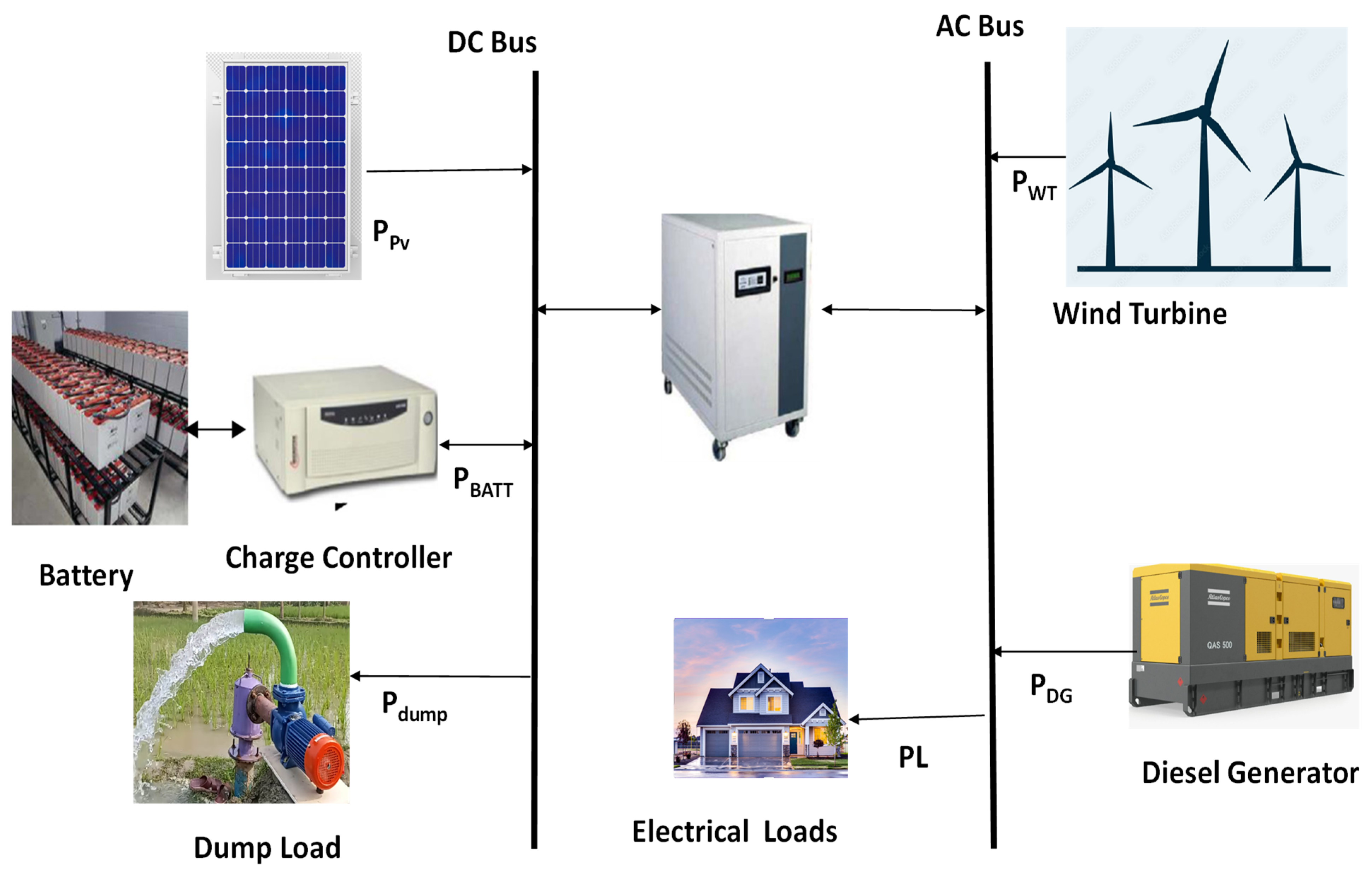
2.1. Components of a Microgrid

MGs, decentralized energy systems, are significantly impacting electricity delivery and consumption by enabling local generation and load management, facilitating the integration of DREs, and enhancing grid resilience. In this section, we investigate the essential components that work together to create a self-sufficient and intelligent power system.

Generation Sources: MGs integrate two primary types of generation sources: dispatchable and non-dispatchable sources. Dispatchable sources, such as natural gas generators and combined heat and power units, can be turned on or off to meet fluctuating electricity demand. Conversely, non-dispatchable sources, such as solar, wind, hydro, and biofuels, rely heavily on weather conditions and cannot be easily controlled to match immediate electricity requirements [17].

Energy Storage Systems (ESSs): ESSs serve as vital components within MGs, performing numerous essential functions. They act as buffers to ensure consistent power quality by mitigating fluctuations and dips in electricity supply. Furthermore, ESSs aid in managing peak demand by “shaving” energy usage during high-consumption periods, thereby enhancing efficiency and potentially lowering energy costs for the MGs [18]. In essence, ESSs play a crucial role in maintaining operational stability, a reliable power supply, and the efficient utilization of renewable energy resources.

Electrical Loads: MGs supply two principal categories of electrical loads: critical and deferrable loads. Critical loads are essential for public safety and well-being and must be prioritized at all times. Examples include hospitals, data centers, and emergency response facilities. MGs design ensures a reliable and uninterrupted power supply for these critical loads, even during outages or islanding from the main grid. Unlike critical loads, deferrable loads are non-essential and can be adjusted or temporarily suspended to maintain MG stability and optimize power generation economics. Examples include electric vehicle charging stations, irrigation pumps, and air conditioning systems. By strategically managing deferrable loads, the MG control system can maximize resource efficiency while potentially reducing energy costs. MGs provide reliable and cost-effective power solutions for homes, businesses, and communities by prioritizing critical loads and strategically managing deferrable loads.

Energy Management System (EMS): The EMS acts as the intelligent control center of a microgrid. It utilizes data collected from energy meters and communication tools to make real-time decisions about power generation and load distribution. This decision-making process considers both economic and reliability factors [19]. The EMS is akin to the brain of the MG. It continuously monitors energy production from various sources, analyzes power consumption demands, and directs the system accordingly. Its goal is to optimize the entire MG operation, balancing two key objectives.

Economic Efficiency—The EMS aims to generate and distribute power in the most cost-effective way possible. This may involve factors such as fuel prices and time-of-use electricity rates, as well as maximizing the use of renewable energy sources.

Reliability—Ensuring a reliable and uninterrupted power supply is paramount. The EMS considers factors such as weather forecasts, potential equipment failures, and grid stability to maintain a constant flow of electricity within the MG.

The EMS optimizes MG performance by addressing economic and reliability aspects, ensuring efficient power generation, cost-effectiveness, and reliable electricity delivery to users.

This study examines a stand-alone MG using two renewable sources (PV and WT), driven by the growing deployment of RES capacity to minimize carbon footprints [20], an energy storage unit (battery), a backup diesel generator, and two types of loads. The MG features a DC bus, where the PV system, dump load and battery are connected via bidirectional converters. The wind turbine, diesel generator, and loads, are directly connected to the single-phase AC bus. As depicted in Figure 1, this low-voltage distribution network operates at 220 V and 50 Hz, supplying power to a single-phase AC and a dump load of DC system.

2.2. Modeling of a Hybrid Microgrid

2.2.1. Photovoltaic Array

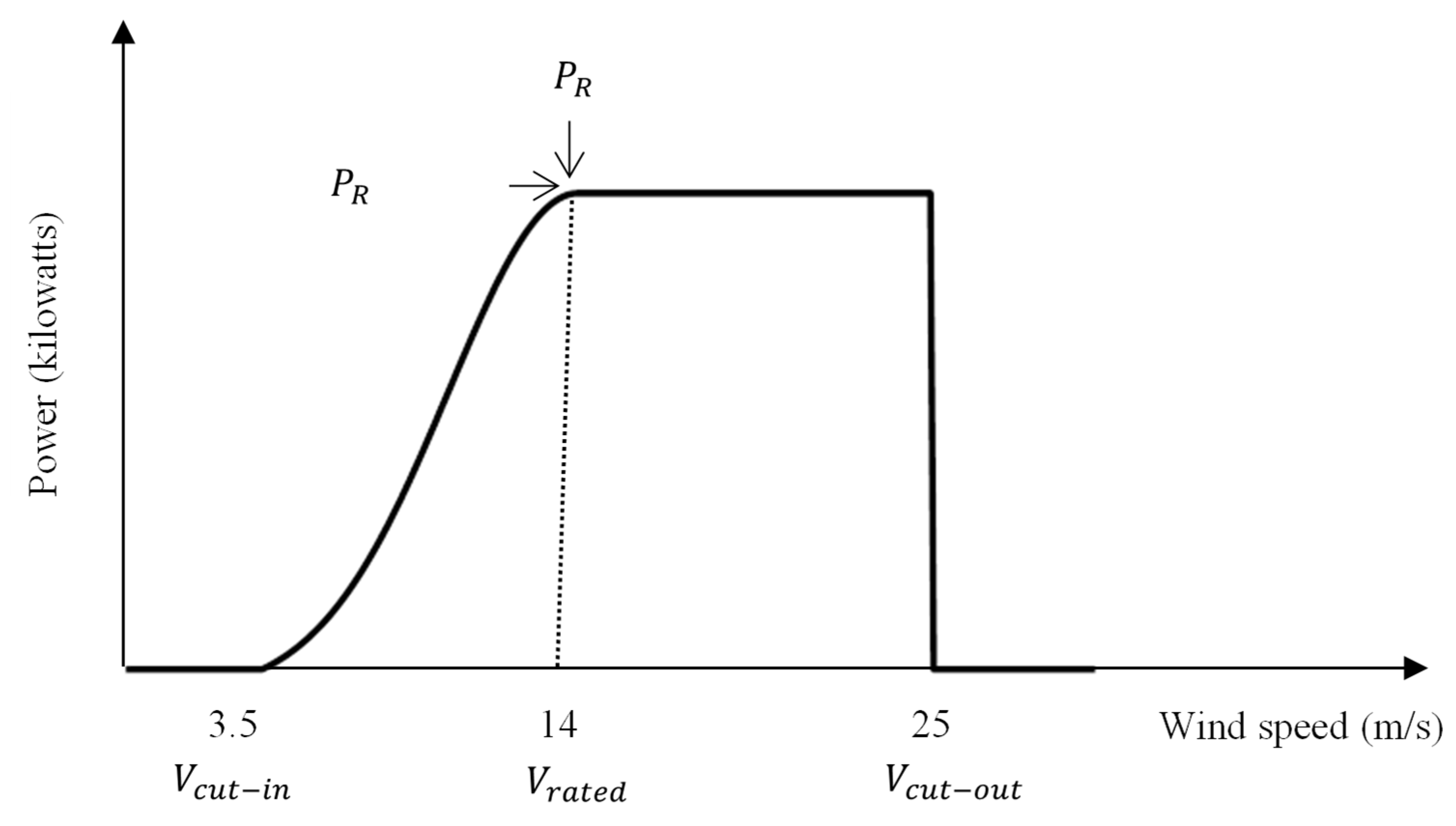
Solar energy is a highly promising renewable resource, with PV systems playing a central role in harnessing this potential [21]. The performance and output of PV systems have been extensively studied in the literature. The energy output of a PV panel is influenced by several factors, including construction density, shading from vegetation or neighboring buildings, and maintenance practices, particularly the accumulation of dust on the panels [22]. The output of PV panel is also influenced by amount of solar irradiation that it receives [23]. This irradiation level is determined by various factors, including local climate conditions, the installation method, and the module type [24]. Individual PV cells are connected in series to form a string in order to achieve the desired output voltage. Conversely, multiple strings are connected in parallel to enhance the output current capacity. This arrangement results in a complete PV panel or module, whose output power rating is calculated by multiplying the output voltage and current [14,25,26]. The output of a PV system can be estimated by considering its rated power, actual irradiance, and ambient temperature [27] as

$$P_{PV}(t)=P_{ref}\times {\displaystyle \frac{G\left(t\right)}{G_{ref}}}\times \left[1+{\alpha }_t\left(T_C\left(t\right)-T_{Cref}\right)\right],$$

(1)

where $P_{PV}\left(t\right)$ is the output power of the PV module in Watts (W); $P_{ref}$ is the rated power of the PV module under standard test conditions in Watts (W); $G\left(t\right)$ is the real solar irradiance in Watts per square meter (W/m²) on the tilted surface of the PV panels; $G_{ref}$ is the standard solar irradiance, typically 1000 watts per square meter (1000 W/m²); $T_{Cref}$ is the standard test condition temperature, usually 25 degrees Celsius (°C); ${\alpha }_t$ is the temperature coefficient of the PV module, typically around −3.7 × 10⁻³ (1/°C) for the mono- and polycrystalline (Si) solar cells [28]; and $T_{amb}$ is the ambient temperature (°C).

$$T_C\left(t\right)=T_{amb}\left(t\right)+\left(0.0256\times G\left(t\right)\right),$$

(2)

Figure 2 demonstrates the relationship between solar irradiance and the performance of the PV array, emphasizing key trends such as voltage, current, and power output across varying irradiance levels.

2.2.2. Wind Turbine

The output power of a WT generator is directly dependent on the wind speed at its hub height. In real-world applications, the location of the WT is of critical importance, as it must be positioned away from obstacles such as buildings, trees, or uneven terrain that could interfere with wind flow and adversely affect its performance. The wind speed can be estimated from the measured wind speed at the anemometer height using a power law [29,30,31]. The turbine’s power output is modeled as a piecewise function, with different equations governing wind speed intervals. When the wind speed reaches the cut-in speed, the turbine generates electricity. The wind density determines the output power, blade swept area, and efficiency coefficient. Once the rated speed is reached, the turbine produces its maximum rated power. If the wind speed exceeds the cut-out speed, then the turbine is shut down for safety. A mathematical representation of the wind speed profile using a power law is given in [32,33]:

$${\displaystyle \frac{V_2}{V_1}}={\left({\displaystyle \frac{h_2}{h_1}}\right)}^{\gamma },$$

(3)

where $V_1$ is the wind speed at the reference height $h_1$ (m/s), $V_2$ is the speed at the hub height $h_2$ (m/s), and $\gamma$ denotes the friction coefficient. $\gamma$ is influenced by various factors such as wind speed, terrain roughness, height above ground, temperature, time of day, and year. While it can vary, the commonly accepted values are 0.11 for extreme wind conditions and 0.2 for normal conditions, according to IEC 61400-1 [34,35]. However, a value of 1/7 is frequently used in practice [27]. The output power of the WT generator is determined by using the following equation [36,37,38]:

$$\begin{array}{l}{P}_{WT}\left(t\right)\\ =\left\{\begin{array}{ccc}0& ,& V\le V_{cut-in}\\ V^3\left({\displaystyle \frac{P_r}{V_{rated}^3-V_{cut-in}^3}}\right)-P_r\left({\displaystyle \frac{V_{cut-in}^3}{V_{rated}^3-V_{cut-in}^3}}\right)& ,& V_{cut-in}<V<V_{rated}\\ P_r& ,& V_{rated}\le V\le V_{cut-out}\\ 0& ,& V\ge V_{cut-out}\end{array},\right.\end{array}$$

(4)

where $P_r$ is the rated power (kW); $V$ is the wind speed (m/s); and $V_{cut-in}$, $V_{rated}$, and $V_{cut-out}$ denote the cut-in, rated, and cut-out wind speed (m/s) of the WT, respectively.

$P_r$ of the wind turbine generator can be expressed as a function of the area swept by the blades $A_{wind}$, the maximum power coefficient $C_p$, the air density ${\rho }_{air}$, and the rated wind speed, as described in [38].

$$P_r={\displaystyle \frac{1}{2}}{C}_p\times {\rho }_{air}\times A_{wind}\times V_{rated}^3$$

(5)

We can also use the cut-in ratio (CIR) to calculate the output of the WT. The CIR is a dimensionless number that represents the ratio of the cut-in wind speed ($V_{cut-in}$) to the rated wind speed ($V_{rated}$) as follows:

$$CIR={\displaystyle \frac{V-V_{cut-in}}{V_{rated}-V_{cut-in}}}$$

(6)

Equation (7) presents the CIR-based model for the wind turbine power output [39,40]. This is utilized to model the output of the WT in this study as

$$P_{WT}\left(t\right)=\left\{\begin{array}{ccc}0& ,& 0\le V\le V_{cut-in}\\ P_r\times CIR& ,& V_{cut-in}\le V\le V_{rated}\\ P_r& ,& V_{rated}\le V\le V_{cut-out}\\ 0& ,& V\ge V_{cut-out}\end{array}\right.$$

(7)

Figure 3 highlights the relationship between wind speed and the WT’s power generation, showcasing how power output increases with wind speed up to the rated capacity and stabilizes thereafter.

2.2.3. Diesel Generator

The DGs function as a backup power source when renewable energy and battery storage are insufficient to meet the load demand. The following equation determines the hourly fuel consumption of the DG [39,40]:

$$F_{DG}\left(t\right)=\alpha P_{DG}\left(t\right)+\beta P_{DGR},$$

(8)

where $F_{DG}\left(t\right)$ represents the fuel consumption of the generator (L/hr), $P_{DG}\left(t\right)$ denotes the generated power (kW), $P_{DGR}$ is the generator’s capacity (kW), $\alpha$ is the fuel curve slope coefficient (L/hr/kW_output), and $\beta$ is the fuel intercept coefficient (L/hr/kW_rated). In this study, the $\alpha$ and $\beta$ values are set to 0.246 and 0.08415, respectively [39,40]. The DG’s fuel cost $C_{DG}\left(t\right)$ is described by

$$C_{DG}\left(t\right)=C_f\sum _{t=1}^{t=8760}{F}_{DG}\left(t\right)$$

(9)

2.2.4. Battery Bank

In a standalone microgrid, the battery system plays a pivotal role by ensuring continuous power delivery to the load, even during periods of insufficient renewable energy generation. The battery capacity can be determined using the following formula [41,42]:

$$C_{BATT}={\displaystyle \frac{AD\times P_{Load}}{{\eta }_{INV}\times {\eta }_{BATT}\times DOD}},$$

(10)

where $P_{Load}$ represents the load power demand; ${\eta }_{INV}$ and ${\eta }_{BATT}$ denote the efficiencies of the inverter and the battery, respectively; $DOD$ signifies the battery depth of discharge; and $AD$ refers to the autonomy days, which is the duration (in days) for which the battery can sustain the load’s power demand before complete depletion.

Renewable energy sources (PV and WT) are inherently intermittent, with their energy output depending on wind speed and solar radiation. To address potential power deficits from these sources, autonomy days are crucial for sizing the battery bank. Excess energy can be accumulated within the battery for future consumption. The power output from the battery bank is calculated as follows [43]:

$$P_{BATT}\left(t\right)=\left[P_{PV}\left(t\right)+P_{WT}\left(t\right)\right]-{\displaystyle \frac{P_{Load}\left(t\right)}{{\eta }_{INV}}},$$

(11)

where $P_{PV}\left(t\right)$, $P_{WT}\left(t\right)$, and $P_{Load}\left(t\right)$ denote the power outputs of the PV, WT, and load power demand, respectively.

A negative $P_{BATT}\left(t\right)$ value signifies an energy generation deficit, while a positive value indicates surplus energy. When $P_{BATT}\left(t\right)$ equals zero, the renewable energy generation perfectly matches the load demand. Evaluating a battery bank’s condition critically relies on its state of charge (SOC), a key indicator that mirrors its current capacity and directly impacts its performance. The SOC can be determined by analyzing both charging and discharging cycles [40,41]:

Charging cycle: when $P_{PV}\left(t\right)+P_{WT}\left(t\right)>P_{Load}\left(t\right)$,

$$SOC\left(t\right)=SOC\left(t-1\right)\times \left(1-\sigma \right)+\left(\left(P_{PV}\left(t\right)+P_{WT}\left(t\right)\right)-{\displaystyle \frac{P_{Load}\left(t\right)}{{\eta }_{INV}}}\right)\times {\eta }_{BATT}$$

(12)

Discharging cycle: when $P_{PV}\left(t\right)+P_{WT}\left(t\right)<P_{Load}\left(t\right)$,

$$SOC\left(t\right)=SOC\left(t-1\right)\times \left(1-\sigma \right)+\left({\displaystyle \frac{P_{Load}\left(t\right)}{{\eta }_{INV}}}-\left(P_{PV}\left(t\right)+P_{WT}\left(t\right)\right)\right)\times {\eta }_{BATT}$$

(13)

2.2.5. Power Converter Modeling

Power conversion is essential in systems with both AC and DC components. Solar PV panels and batteries generate DC power, while many loads operate on AC. DC/AC and AC/DC power converters are necessary to interface these components. The peak load demand determines the size of these converters. The inverter rating is calculated as follows:

$$P_{INV}\left(t\right)={\displaystyle \frac{P_{Load}^m\left(t\right)}{{\eta }_{INV}}},$$

(14)

where $P_{INV}\left(t\right)$ is the inverter rating, and $P_{Load}^m\left(t\right)$ is the peak load demand.

2.3. Objective Functions

The sizing optimization of HESs prioritizes minimizing cost while maintaining reliable power delivery. This inherently involves trade-offs, with system investment and reliability being key considerations. This study employs the ACS and the LPSP as the primary objective functions to quantify these competing goals.

2.3.1. Annualized Cost of System

To calculate the annualized cost of a HESs, it is essential to conduct a thorough assessment of the initial investment costs; ongoing expenses, such as replacement, operation, and maintenance costs; and fuel costs of each component.

The levelized cost of energy (LCOE) is a critical metric used to evaluate the economic viability of long-term energy projects, providing a standardized measure of the average cost per unit of electricity generated over the project’s lifespan. It denotes the cost per unit of energy generated by the HES (measured in USD/kWh). The following equations can be employed to evaluate the LCOE of each component within the MGs [14,44]:

$$C_{PV}=N_{PV}\left[I{C}_{PV}+CO\&M_{PV}\times CRF\right],$$

(15)

$$C_{WT}=N_{WT}\left[I{C}_{WT}+CO\&M_{WT}\times CRF\right],$$

(16)

$$C_{BATT}=N_{BATT}\left[I{C}_{BATT}+CO\&M_{BATT}\times CRF\right]+R{C}_{BATT}\times \sum _{j=1}^{{\displaystyle \frac{n}{n_{BATT}}}-1}\left(1+{\displaystyle \frac{1}{\begin{array}{c}{\left(1+i\right)}^{n_{BATT}}\end{array}}}\right),$$

(17)

$$C_{DG}=N_{DG}\left[I{C}_{DG}+CO\&M_{DG}\times CRF\right]+R{C}_{DG}\times {\sum }_{j=1}^{{\displaystyle \frac{n}{n_{DG}}}-1}\left(1+{\displaystyle \frac{1}{\begin{array}{c}{\left(1+i\right)}^{n_{DG}}\end{array}}}\right),$$

(18)

$$C_{INV}=P_{INV}\left[I{C}_{INV}+CO\&M_{INV}\times CRF\right],$$

(19)

$$CRF={\displaystyle \frac{i\times {\left(1+i\right)}^n}{\begin{array}{c}{\left(1+i\right)}^n-1\end{array}}},$$

(20)

where $C_{PV}$, $C_{WT}$, $C_{BATT}$, $C_{DG}$, and $C_{INV}$ are the energy costs of the PV system, WT system, battery bank, diesel generator, and inverter, respectively; $I{C}_{PV}$, $I{C}_{WT}$, $I{C}_{BATT}$, $I{C}_{DG}$, and $I{C}_{INV}$ represent the costs invested into these sources of energy, respectively; $CO\&M_{PV}$, $CO\&M_{WT}$, $CO\&M_{BATT}$, $CO\&M_{DG}$, and $CO\&M_{INV}$ are the operation and maintenance costs of the PV, WT, battery bank, DGs, and inverter, respectively; $R{C}_{BATT}$ and $R{C}_{DG}$ are the replacement costs of the battery bank and the DG, respectively; $i$ is the annual interest; $n$ is the system lifetime; $n_{BATT}$ and $n_{DG}$ are the lifetime of the battery bank and the diesel generator, respectively; and $CRF$ is the capital recovery factor.

The calculation of the net cost of the four sources proceeds as follows:

$$ASC=C_{PV}+C_{WT}+C_{BATT}+C_{DG}+C_{INV}$$

(21)

The LCOE is given by

$$LCOE=ASC\times CRF\times {\displaystyle \frac{1}{\sum _{h=1}^{8760}{P}_G}},$$

(22)

where $P_G$ is the hourly power generation.

2.3.2. Loss of Power Supply Probability

The LPSP is a statistical metric assessing the risk of a power system failing to meet the electricity demand at a given point. This value falls between 0 and 1, where 0 represents perfect reliability, and 1 signifies complete unreliability. Factors influencing the LPSP include system capacity, load demand, component reliability, maintenance schedules, and natural disasters. The LPSP analysis is crucial for various applications, such as MG design, power system planning, renewable energy integration, and emergency response planning. By understanding the probability of power outages, engineers and policymakers can make informed decisions to enhance the reliability and resilience of power systems [45].

$$LPSP={\displaystyle \frac{\sum _{t=1}^{8760}\left[P_{Load}\left(t\right)-P_G\left(t\right)\right]}{\sum _{t=1}^{8760}{P}_{Load}\left(t\right)}},$$

(23)

where $P_{Load}\left(t\right)$ and $P_G\left(t\right)$ are the hourly load demand and the hourly system output or generation, respectively.

2.4. Constraints

The renewable factor (RF) is a metric used to assess the extent to which a microgrid relies on renewable energy sources. It quantifies the proportion of power generated from renewable resources (such as solar and wind) compared to non-renewable sources (such as DGs). This factor is expressed as follows [46]:

$$RF=1-{\displaystyle \frac{\sum P_{DG}}{\sum P_{PV}+\sum P_{WT}}}\times 100\%$$

(24)

An RF of 100% signifies that the system is entirely powered by renewable energy sources, representing an ideal scenario of complete reliance on clean energy. Conversely, RF of 0% indicates that the power from renewable sources exactly matches the power supplied by the diesel generator, implying an equal contribution from both renewable and non-renewable sources.

2.4.1. Design Variables

This study investigates the impact of four design variables: the number of PV modules ($N_{PV}$), WT ($N_{WT}$), DGs ($N_{DG}$), and battery systems ($N_{BATT}$). The constraints associated with these proposed design variables are outlined as follows:

$$\begin{array}{ccccc}1& \le & N_{PV}& \le & N_{PV}^{max}\\ 1& \le & N_{WT}& \le & N_{WT}^{max}\\ 1& \le & N_{DG}& \le & N_{DG}^{max}\\ 1& \le & N_{BATT}& \le & N_{BATT}^{max}\end{array}$$

(25)

2.4.2. Generation Unit Boundaries

The output of each generation unit must fall within the prescribed range, defined by the minimum and maximum permissible values [39]:

$$\begin{array}{ccccc}{P}_{PV}^{min}& \le & P_{PV}\left(t\right)& \le & P_{PV}^{max}\\ P_{WT}^{min}& \le & P_{WT}\left(t\right)& \le & P_{WT}^{max}\\ P_{DG}^{min}& \le & P_{DG}\left(t\right)& \le & P_{DG}^{max}\end{array}$$

(26)

2.4.3. Supply–Demand Balance

The microgrid system must maintain power output in continuous equilibrium with the fluctuating load demand [43]:

$$P_G\left(t\right)=P_l\left(t\right)$$

(27)

2.4.4. Battery Storage System (BSS) Constraints

The state of charge (SOC) of the BSS consistently falls within the established minimum and maximum thresholds, expressed as follows [43]:

$$SO{C}_{min}\le SOC\left(t\right)\le SO{C}_{max}$$

(28)

$$SO{C}_{min}=\left(1-DOD\right)\times SO{C}_{max}$$

(29)

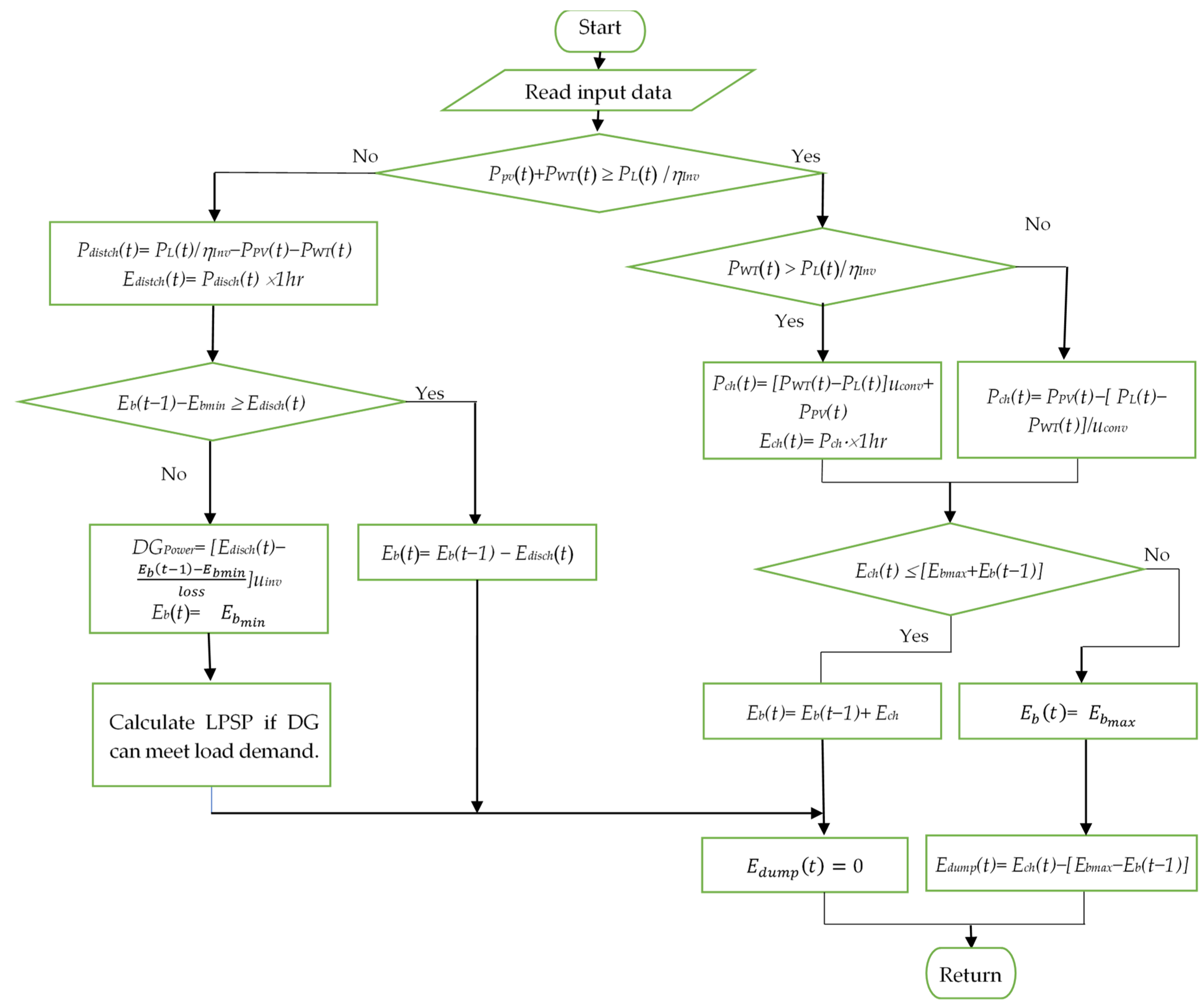
2.5. Energy Management Strategy of Hybrid Microgrid System

Hybrid microgrids elegantly combine diverse energy sources, such as renewable power (solar and wind), traditional generators, and energy storage (batteries). A robust EMS is essential to ensure dependable and efficient power delivery. The key objectives of an effective EMS include the following:

• Maximize renewable energy utilization by prioritizing clean and sustainable energy sources to reduce fossil fuel dependence and minimize greenhouse gas emissions.
• Minimize operating costs by optimizing renewable energy source operation to reduce fuel consumption and maintenance costs.
• Ensure power quality by maintaining the voltage and frequency within acceptable limits to guarantee quality power supply to the load.
• Enhance system reliability by developing strategies to mitigate the impact of intermittent renewable energy sources and ensure an uninterrupted power supply.
• Optimize energy storage system operation by managing ESS charging and discharging to maximize utilization and lifespan.

In this study, four energy management scenarios are implemented:

• Scenario 1: Renewable energy sources (PV and WT) generate sufficient power to meet the load demand ($P_{Load}$). Excess energy is stored in the battery bank or used to charge the battery ($P_{ch}$); this is given by $P_{ch}\left(t\right)=\left[P_{WT}\left(t\right)-P_L\left(t\right)\right]u_{conv}+P_{PV}\left(t\right)$ if the wind turbine power exceeds the load power and by $P_{ch}\left(t\right)=P_{PV}\left(t\right)-\left[P_L\left(t\right)-P_{WT}\left(t\right)\right]/u_{conv}$ if it does not exceed it, where $u_{conv}$ is the converter efficiency.
• Scenario 2: When renewable energy generation exceeds the load demand and the battery is fully charged, surplus energy is dissipated through a dump load $E_{dump}$.
• Scenario 3: If renewable energy generation falls short of the load demand, the battery bank ($P_{disch}$) supplies the deficit to meet the load requirement. This is given by $P_{disch}\left(t\right)=P_L\left(t\right)/{\eta }_{INV}-P_{PV}\left(t\right)-P_{WT}\left(t\right)$.
• Scenario 4: When renewable energy generation is insufficient to meet the load demand and the battery bank’s storage level is low, the DG operates to cover the deficit and recharge the battery bank.

Figure 4 illustrates a flowchart of the operating strategy of the proposed hybrid energy system. In the figure, $E_b\left(t\right)$ represents the battery energy at time $t$; $E_{bmax}$ and $E_{bmin}$ are the maximum and minimum battery energy, respectively, which are related using (29); and $E_{ch}\left(t\right)$ and $E_{disch}\left(t\right)$ denote the charging and discharging energy, respectively.

3. Optimization of Hybrid Microgrids

3.1. Non-Dominated Sorting Genetic Algorithm II (NSGA-II)

With the surge in the demand for sustainable energy solutions, HMGs have emerged as a promising approach to enhance energy resilience, reduce carbon emissions, and improve overall system efficiency. However, designing and operating these complex systems require careful consideration of multiple, often conflicting, objectives. This is where NSGA-II comes into play. NSGA-II is a popular and powerful metaheuristic algorithm used to solve multi-objective optimization problems. It is designed to find a diverse set of solutions that efficiently balance multiple conflicting objectives. The key features of NSGA-II are as follows:

• Non-Dominated Sorting: NSGA-II employs a fast, non-dominated sorting approach to rank solutions based on their dominance relationships. Solutions that are not dominated by any other solution are assigned to the first front, and the process continues iteratively.
• Crowding Distance: To maintain diversity among solutions, NSGA-II calculates the crowding distance for each solution. This metric measures the density of solutions in the objective space. Solutions with higher crowding distances are more likely to be selected for the next generation, ensuring a well-distributed Pareto front.
• Elitism: NSGA-II incorporates an elitism mechanism to preserve the best solutions from the current generation. This helps to maintain the quality of the population over time.
• Genetic Operators: NSGA-II uses standard genetic operators such as crossover and mutation to generate new solutions. These operators help explore the solution space and find better solutions.

More details regarding this algorithm can be found in [47]. The results of an NSGA-II run typically consist of a set of non-dominated solutions, often referred to as the Pareto front. These solutions represent a trade-off between the two objectives being optimized.

3.2. Optimization of Hybrid Microgrid Using the HGA

As previously mentioned, there is an inherent conflict between achieving good ASCs and a reliable LPSP in a HMSs. Each point on the Pareto front represents a non-dominated solution that offers an optimal trade-off between the two conflicting objectives. This means that no other solution exists that can improve one objective without worsening the other. For example, a point on the Pareto front might represent a solution that has moderately high ASCs but offers a highly reliable LPSP. Another point might represent lower ASCs with a lower reliability of the LPSP. The Pareto front helps decision-makers visualize the range of possible solutions and the trade-offs involved. Decision-makers choose a solution that offers an optimal trade-off between the two conflicting objectives.

This process ends up being the same problem as combining two objective functions into a single objective function and then optimizing it. To achieve this, we assign a weight to an objective function as

$$\mathrm{M}\mathrm{i}\mathrm{m}\mathrm{i}\mathrm{m}\mathrm{i}\mathrm{s}\mathrm{e} f\left(\mathit{x}\right)=LPSP\left(\mathit{x}\right)+w·ASC\left(\mathit{x}\right),$$

(30a)

$$s.t. S=\left\{\mathit{x}| x_j^{\left(L\right)}\le x_j\le x_j^{\left(U\right)}\right\} \left(1\le j\le n\right),$$

(30b)

where $f : S \subset {\mathcal{R}}^4\to \mathcal{R}$ is an objective function to be minimized; S is a set of feasible vectors in a search space called the search space; the vector $\mathit{x}={\left[N_{PV}, N_{WT}, N_{DG}, N_{BATT}\right]}^T\in S$; $x_j^{\left(L\right)}$ and $x_j^{\left(U\right)}$ are the lower and upper limits of the $j$th variable, respectively; and $w$ is the weighting coefficient that determines the relative importance of two objective functions. Increasing the weight of one performance might necessitate sacrificing another performance. For this study, $w$ is set to 0.001.

To solve this single-objective function optimization, we use the HGA, which is based on affine combination-based reproduction and non-uniform mutation [48]. Potential solutions in the HGA are represented as real numbers. The HGA is implemented through a three-step process:

Let $\mathit{P}\left(t\right)$ be a population of N individuals at generation t:

$$\mathit{P}\left(t\right)={\left[x_1\left(t\right) \cdots x_i\left(t\right) \cdots x_n\left(t\right)\right]}^T,$$

(31)

where ${\mathit{x}}_i\left(t\right)={\left[N_{i,PV}, N_{i,WT}, N_{i,DG}, N_{i,BATT}\right]}^T\left(1\le i\le N\right)$ is the $i$th individual. The function value $f\left({\mathit{x}}_i\right(t\left)\right)$, simply as $f_i\left(t\right)$, of each individual is evaluated from the objective function.

Step 1. The global best and the local best and worst are determined from the population:

$$f_{best}\left(t\right)=\underset{1\le i\le N}{\min }\left\{f_i\left(t\right)\right\},$$

(32a)

$$f_{worst}\left(t\right)=\underset{1\le i\le N}{\max }\left\{f_i\left(t\right)\right\},$$

(32b)

$$f_{global}\left(t\right)=\underset{1\le i\le N}{\mathit{min}}\left\{f_{best}\left(1\right), f_{best}\left(2\right), \cdots ,f_{best}\left(t\right)\right\},$$

(32c)

$${\mathit{x}}_{global}\left(t\right)=\mathrm{a}\mathrm{r}\mathrm{g}\left\{f_{global}\left(t\right)\right\},$$

(32d)

where $f_{best}\left(t\right)$ and $f_{worst}\left(t\right)$ are the local best and worst function values found in the current population, respectively; ${\mathit{x}}_{global}\left(t\right)$ and $f_{global}\left(t\right)$ are the global best and its function value, respectively, which give the best value ever explored in the population; and t is the current generation. The values found in Equation (32) are used to guide the movement of all individuals towards the global solution.

Step 2. Each individual is updated based on the global best, the local worst, and its own function value. The following formula assigns a new value to the ith individual:

$${\mathit{x}}_i\left(t+1\right)={\mathit{x}}_i\left(t\right)+{\eta }_i{\gamma }_i\left(t\right)\left[{\mathit{x}}_{global}\left(t\right)-{\mathit{x}}_i\left(t\right)\right],$$

(33a)

$${\gamma }_i\left(t\right)={\displaystyle \frac{f_{global}\left(t\right)-f_i\left(t\right)}{f_{global}\left(t\right)-f_{worst}\left(t\right)}},$$

(33b)

where ${\eta }_i$ is a positive constant, empirically chosen to ensure a significant improvement in the performance of the HGA, and ${\gamma }_i\left(t\right)$ is the ratio of the difference between $f_{global}\left(t\right)$ and $f_i\left(t\right)$ to that between $f_{global}\left(t\right)$ and $f_{worst}\left(t\right)$. The value of ${\gamma }_i\left(t\right)$ is between 0 and 1, inclusive. ${\eta }_i$ is sampled from a Gaussian distribution, $N\left(\eta ,{\sigma }^2\right)$, with mean $\eta$ and standard deviation $\sigma$. This results in each individual being assigned a value that is likely to be near $\eta$, with some variation.

Step 3. The formula for reproduction in Equation (34) contributes to exploration by numerically modifying individuals, but mutation plays a critical role not only in introducing genetic diversity but also in preventing the algorithm from converging too quickly to a local optimum. In the HGA, non-uniform mutation is employed. When a gene (or variable) is selected for mutation, it is altered by a random amount, as described in Equation (34) [48]:

$$x_j^{\prime }=\left\{ \begin{array}{cc}{x}_j+\mathsf{\Delta }\left(t, x_j^{\left(U\right)}-x_j\right)& if q=0\\ x_j-\mathsf{\Delta }\left(t, x_j-x_j^{\left(L\right)}\right)& if q=1\end{array}\right.\prime$$

(34a)

$$\mathsf{\Delta }\left(t, y\right)=y\left[1-r^{{\left(1-{\displaystyle \frac{t}{t_{max}}}\right)}^b}\right],$$

(34b)

where $x_j$ is the selected gene, $x_j^{\prime }$ is the result, $q$ is a random digit (0 or 1), $r$ is a uniform random number, $r\in [0,1]$, $t_{max}$ is the maximum number of generations, and $b$ is the shape parameter. The mutation rate $p_m$ governs how frequently mutations occur; a low $p_m$ leads to a more conservative search strategy, whereas a high $p_m$ encourages a more exploratory approach. Additionally, the shape parameter $b$ influences the distribution of mutations: increasing $b$ results in a narrower distribution, while decreasing $b$ produces a broader distribution.

Regarding the parameter settings of the HGA, the population size was set to 40. Previous research results showed good performance at a reproduction constant of $\eta$ = 1.8, with $\sigma$ = 0.01, a mutation rate of $p_m$ = 0.05, and a shape parameter of $b$ = 6 [48].

4. Simulation Results and Discussion

4.1. Case Study Site and System Specifications

This section details the specific site selected for the case study and outlines the technical specifications of the system under investigation.

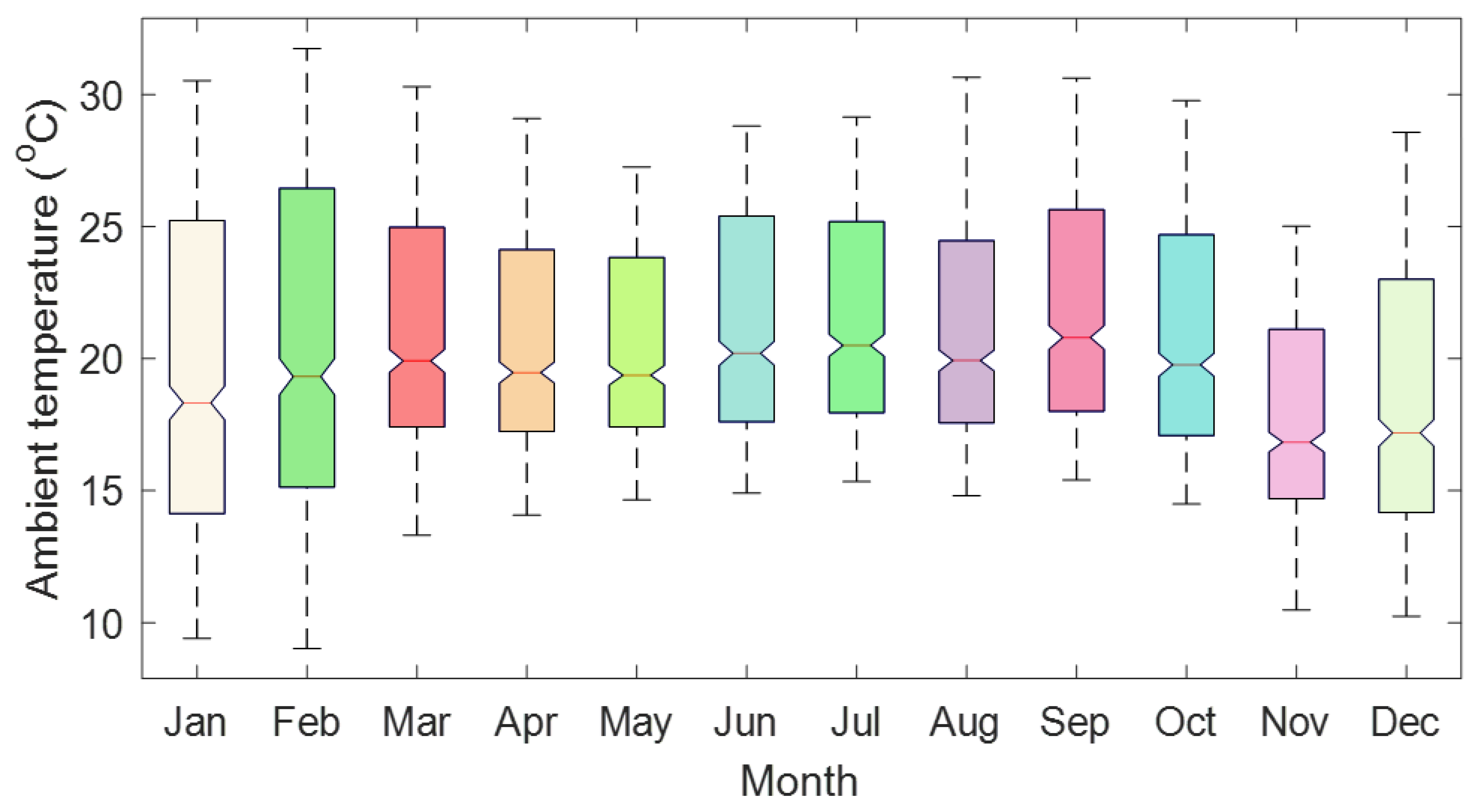
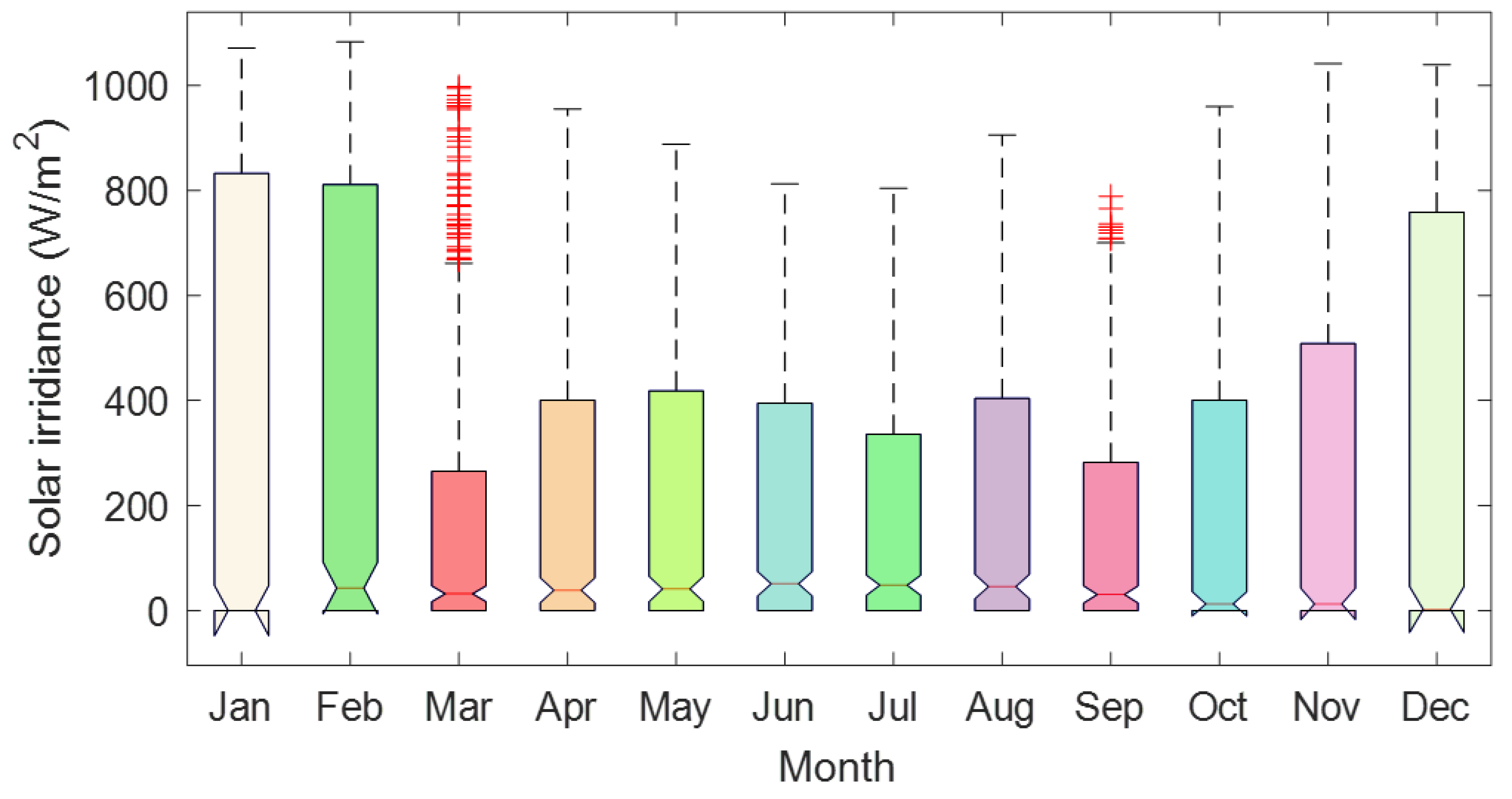
4.1.1. Location and Meteorological Conditions

The proposed standalone MG for the HRES is located at the Adama Science and Technology University, at 8.56295° N and 39.28978° E, in the Oromia region of Ethiopia. Adama is characterized by a semi-arid climate with distinct wet and dry seasons. The average annual temperatures range from approximately 15 °C (59 °F) to 30 °C (86 °F), with warm daytime conditions and cooler nights. Rainfall is concentrated primarily from June to September, peaking in July and August, with annual averages typically between 600 and 800 mm (23 and 31 inches), though this can vary significantly. Humidity levels are generally moderate, increasing during the rainy season. Wind speeds are typically mild but may intensify during specific periods, especially in the dry season. Adama benefits from abundant sunshine, which is ideal for solar power generation. Accurate meteorological data are essential for successful renewable energy projects, especially solar and wind. Wind speed, solar radiation, and ambient temperature data for the simulations were obtained from NASA [49] at the coordinates of Adama city (8.5145° N, 39.2693° E). At the selected location for the specified year, the average solar radiation was 0.2357 kW/m², the average wind speed was 3.206 m/s, and the average ambient temperature was 293.4010 K. Figure 4, Figure 5 and Figure 6 illustrate the hourly solar radiation profile, the wind speed at a height of 10 m above ground level, and the ambient temperature over a year (8760 h).

Figure 7, Figure 8 and Figure 9 display the monthly profiles of solar radiation, wind speed measured at 10 m, and ambient temperature over a year.

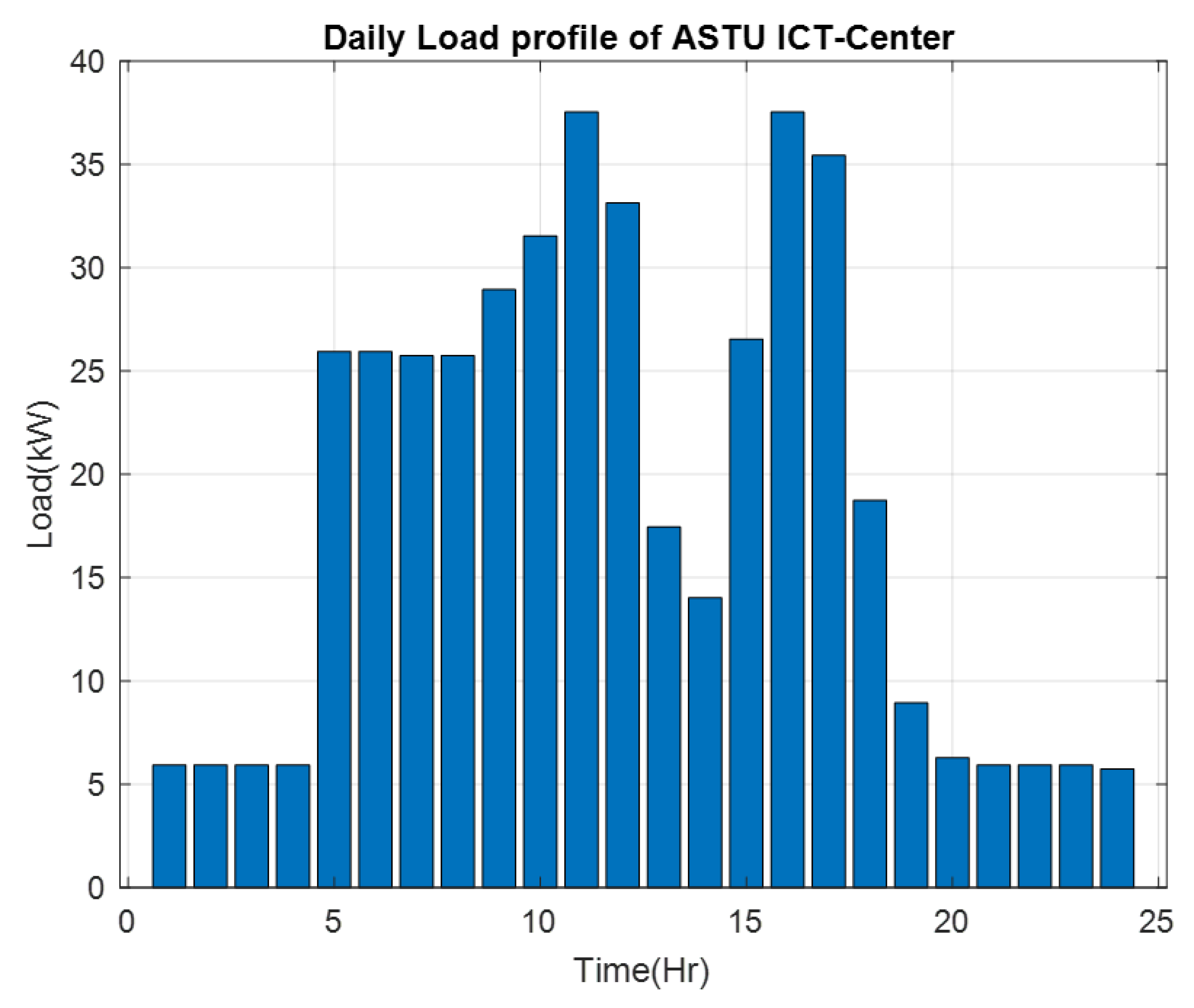
4.1.2. Load Assessment

A load assessment is crucial in designing and sizing standalone MGs powered by renewable energy systems and in analyzing any electrical system. It involves calculating the total power consumption of all electrical devices and equipment within a study area or facility. This research used direct measurement and load estimation methods for load assessments. The type of load considered in this area is given in

Table 1. Analysis of power consumption and appliance utilization at ASTU-ICT center.

Rooms and Load	Qty (pcs)	Rating (W)	Total P (kW)	Hrs./Day	Energy/Day
Office room	12
Lighting	16	25	0.4	1	0.4
Socket outlets	8	50	0.4	1	0.4
Socket outlets	16	50	0.8	6	4.8
Ventilators	8	25	0.2	4	0.8
Refrigerator	8	200	1.6	18	28.8
Printer	8	100	0.8	2	1.6
Scanner	8	50	0.4	1	0.4
Copier	8	1000	8	1	8
Conference room	2
Lighting	8	25	0.2	1	0.2
Socket outlet	4	50	0.2	2	0.4
LCD projector	2	100	0.2	5	1
TV set	2	150	0.3	2	0.6
Air conditioner	4	250	1	5	5
Labs	8
Lighting	64	25	1.6	3	4.8
Socket outlet/PCs	400	50	20	11	220
Projector	8	100	0.8	6	4.8
Air conditioner	16	250	4	6	24
Switches (Nw)	8	25	0.2	24	4.8
Switches (Nw)	4	50	0.2	24	4.8
Server room	1
Lighting	4	25	0.1	3	0.3
Socket outlets	6	50	0.3	4	1.2
Servers	4	500	2	24	48
Ventilators	4	60	0.24	12	2.88
Air conditioner	2	500	1	24	24
Library/smart room	1
Lighting	10	25	0.25	3	0.75
Socket outlets	40	50	2	8	16
Printing	2	100	0.2	2	0.8
Scanner	2	50	0.1	1	0.1
Copier (Xerox)	1	1000	1	1	1
Ventilators	10	60	0.6	8	4.8
Air conditioner	4	250	0.1	7	0.7
TV set (room)	4	150	0.6	4	2.4
TV set corridor	1	500	0.5	24	12
Rest rooms	12
Lighting	24	25	0.6	2	1.2
Socket outlets	12	50	-	-	-
Corridors	12
Lighting	18	25	0.45	1	0.45
Lighting	8	25	0.2	12	2.4
Socket outlets	12	50	-	-	-
Total (kW) = 51.54 kW				Total = 434.58 kWh/d

, and the daily load profile is given in Figure 10.

4.1.3. Specifications of Hybrid Microgrid System Components

To guarantee system reliability, components with adequate rated capacities must be selected to prevent widespread power outages or MGs collapse due to equipment failure.

Table 2. Technical and economic specifications of hybrid microgrid components.

Component/Sources	Parameter	Value	Units
Photovoltaic (PV)	Lifespan	20	Years
	Rated capacity	1	kW
	Efficiency	95	%
	Initial cost	1200	USD/kW
	Running cost	2	%
Wind turbine (WT)	Lifespan	20	Years
	Rated capacity	1	kW
	Efficiency	95	%
	Initial cost	3200	USD/kW
	Running cost	2	%
	Cut-in speed	2.5	m/s
	Cut-out speed	18	m/s
	Rated speed	12	m/s
Diesel generator (DG)	Lifespan	20	Years
	Rated capacity	100	kW
	Efficiency	90	%
	Initial cost	1000	USD/kW
	Fuel cost	1.8	USD/kWh
	Running cost	2	%
Battery storage system (BSS)	Lifespan	5	Years
	Rated capacity	100	kW
	Efficiency	92	%
	Initial cost	750	USD/kW
	Running cost	2	%

presents the economic and technical specifications of the key components.

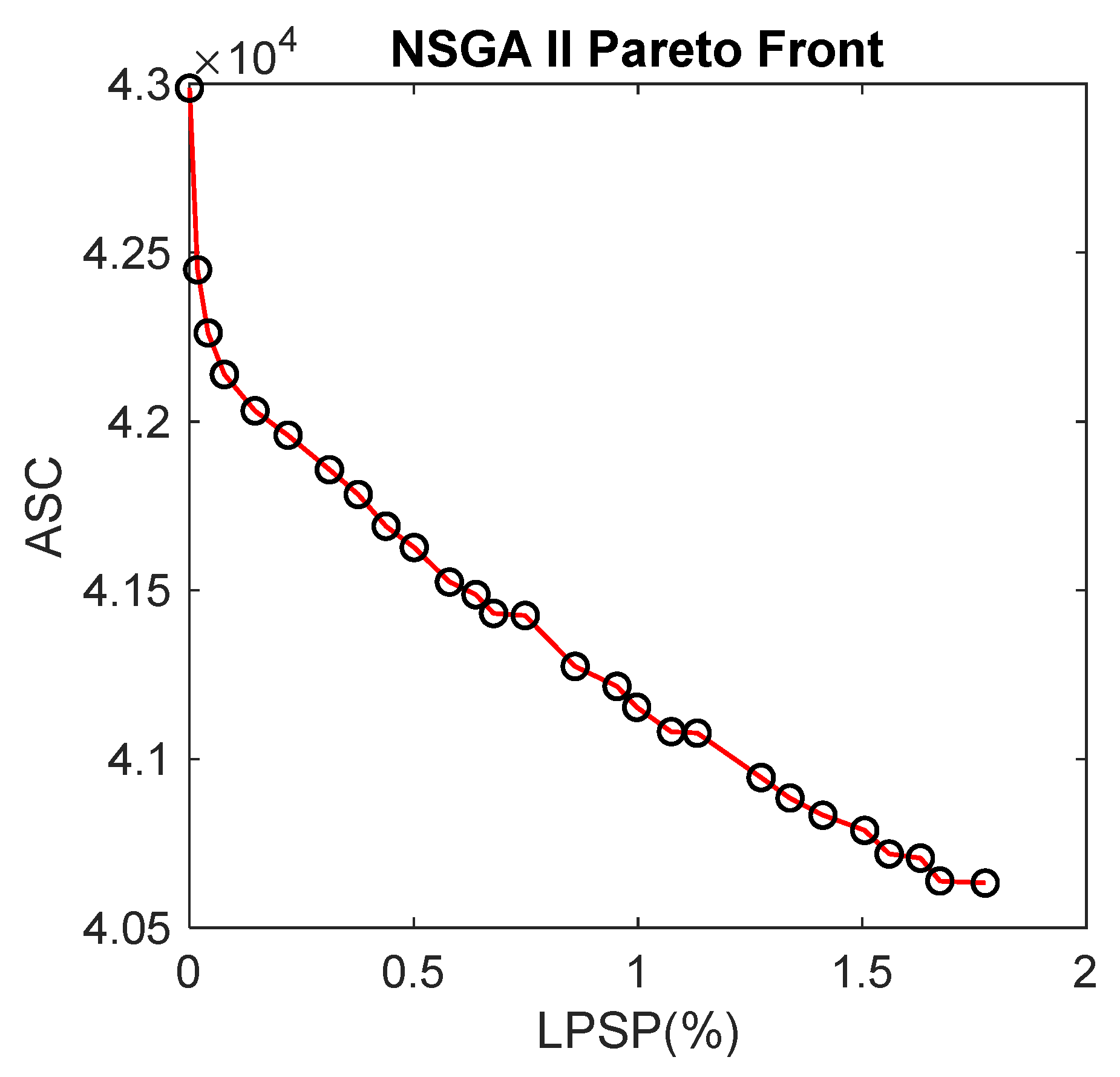
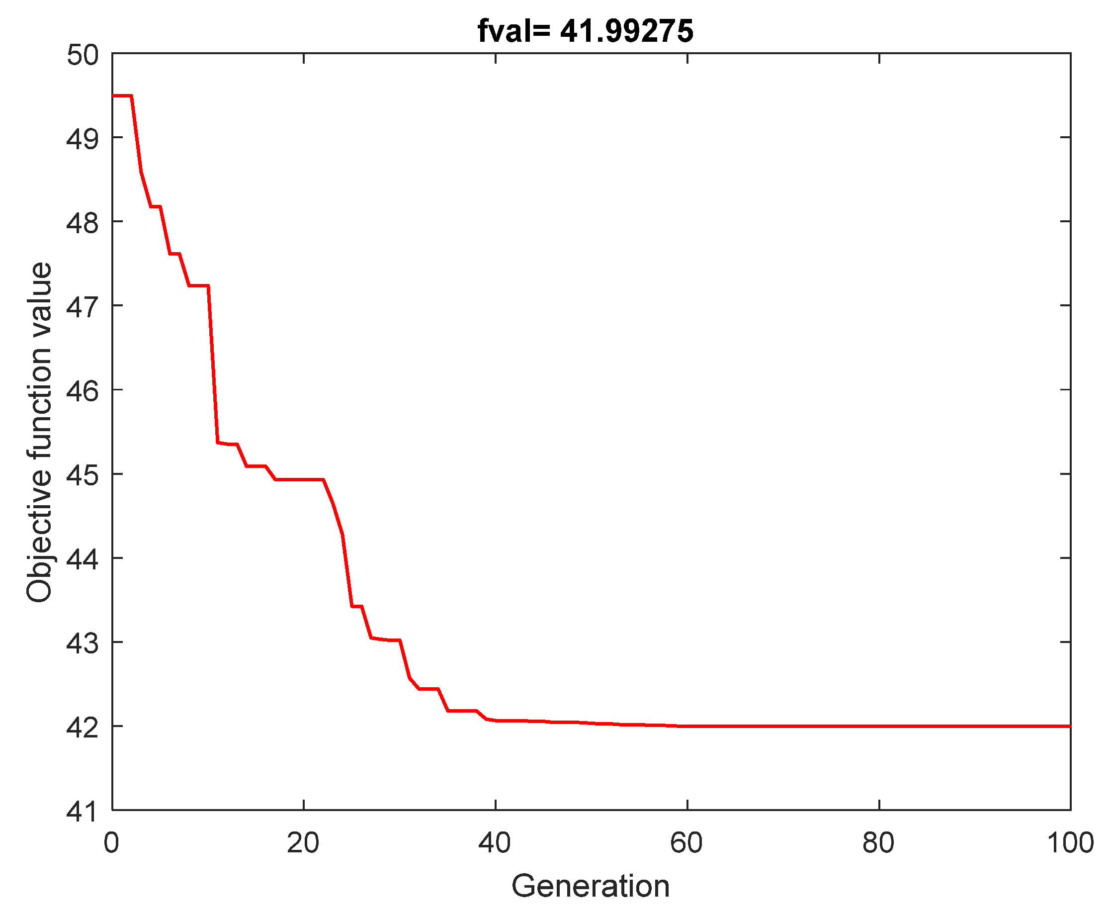
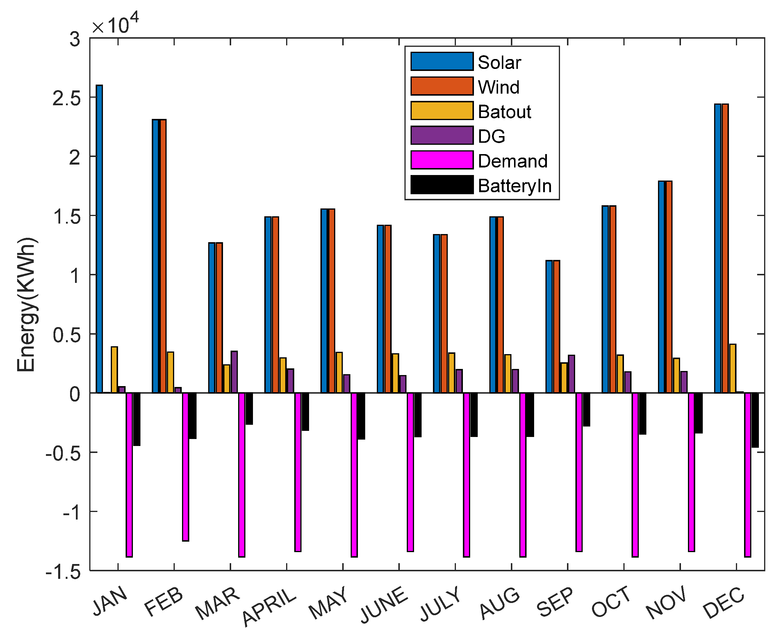
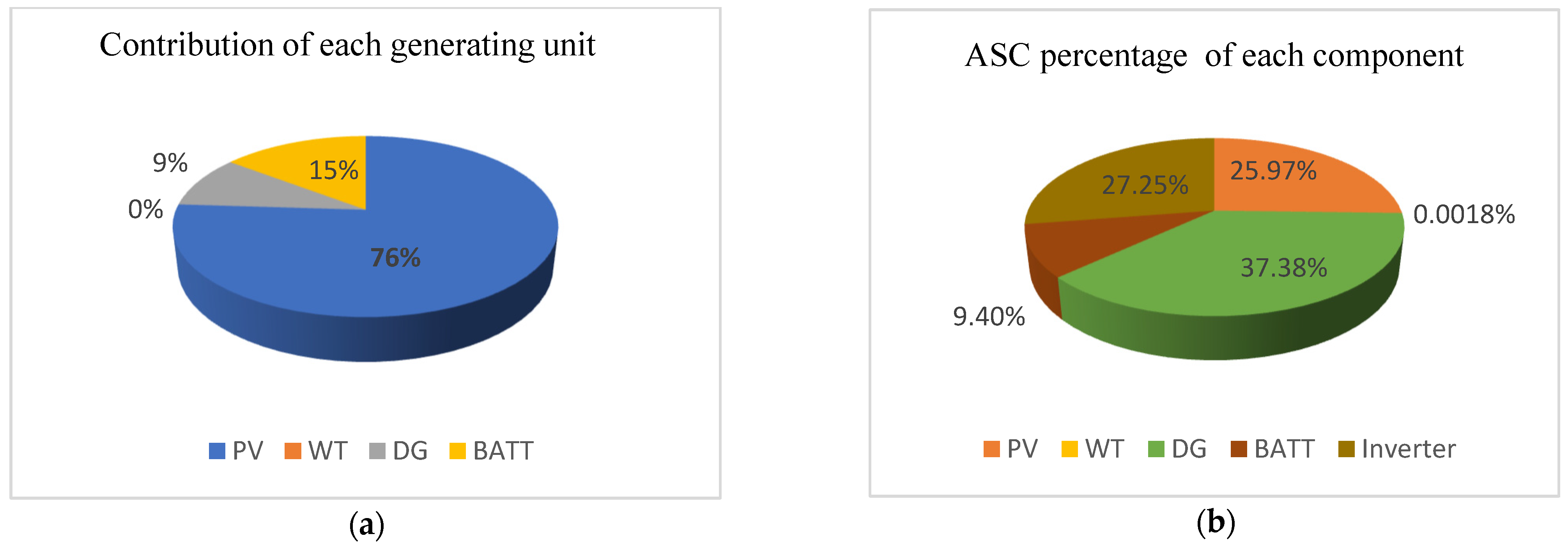
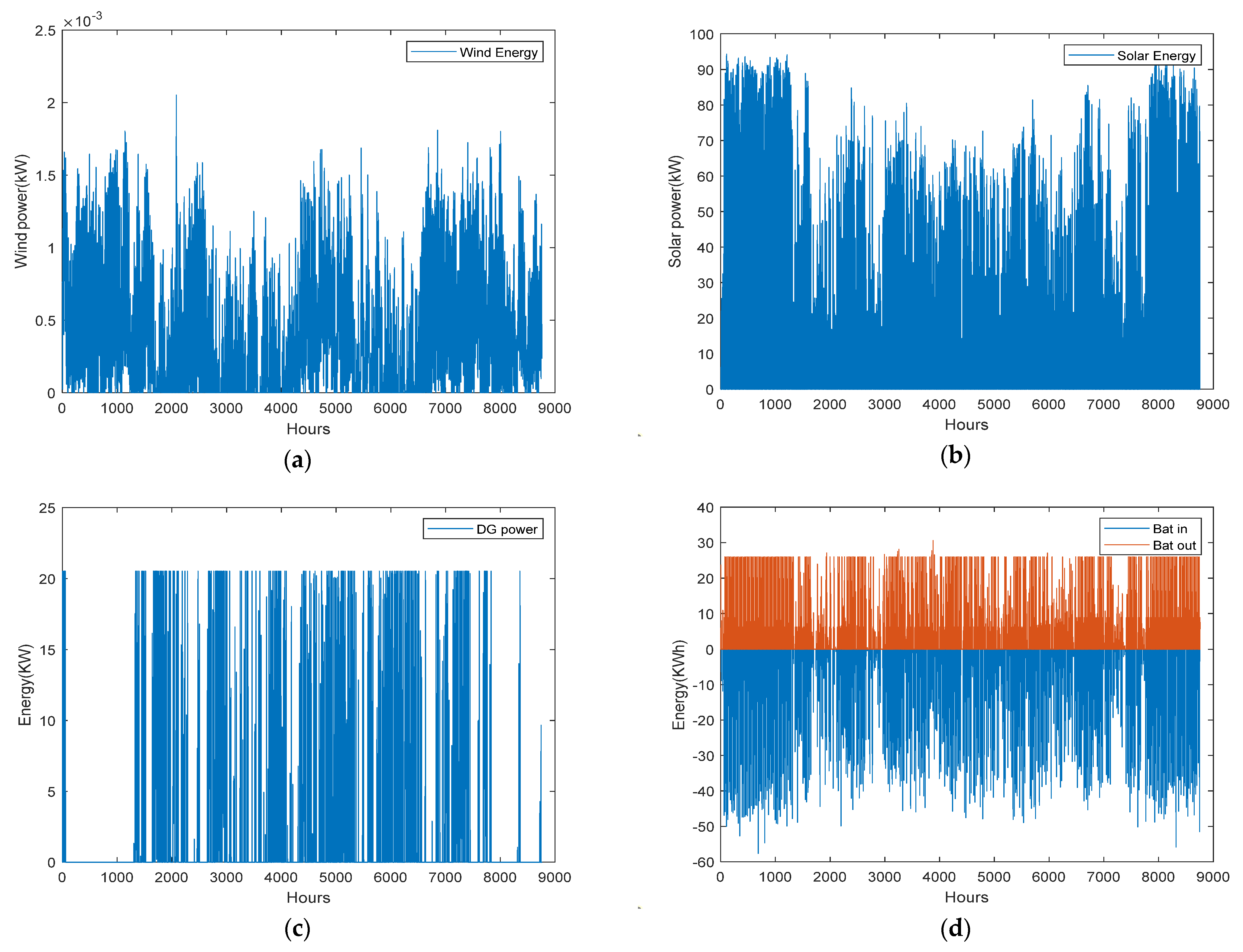
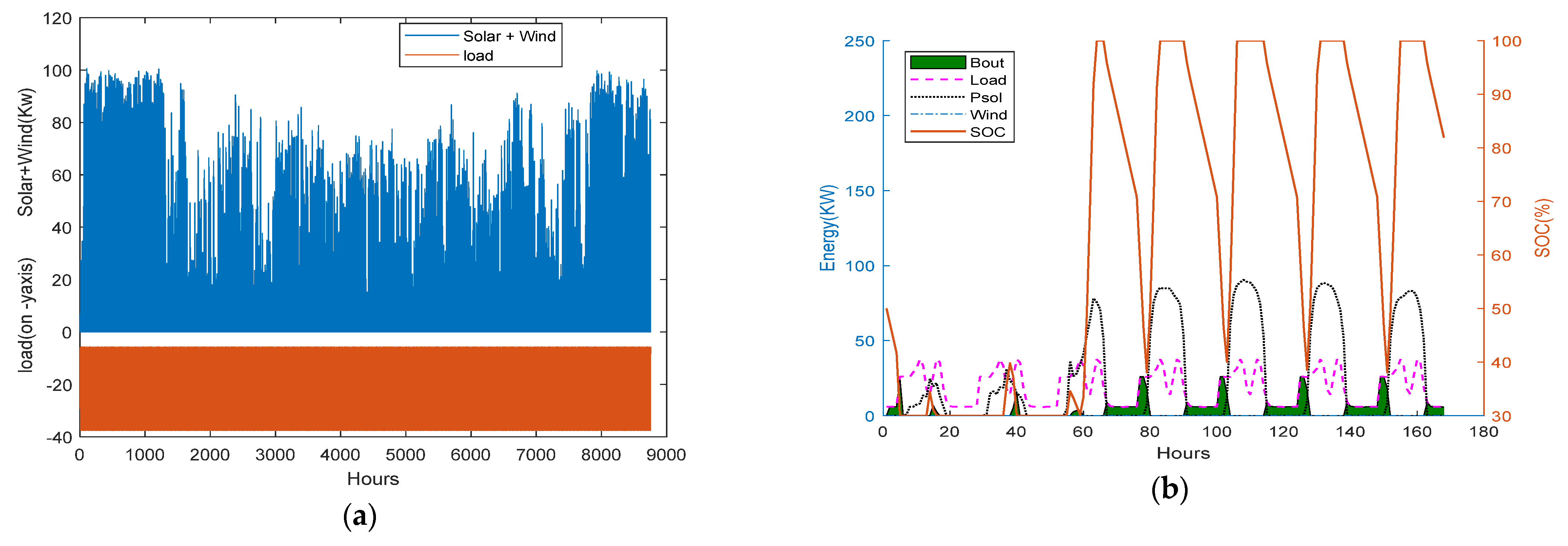
4.2. Results and Discussion

This study presents an optimized design for a standalone HMSs that incorporates PV, WT, a battery bank, and a DG as a backup power source. The primary goal was to meet the energy demand of the ICT center, estimated at 51.4 kW. The HGA was employed to tackle the constrained optimization problem outlined in (30). This study uses a weighting factor value of $w$ = 0.001. The results were compared with those of the MATLAB R2021a particle swarm and genetic algorithm functions. Henceforth, MATLAB particle swarm optimization and the MATLAB genetic algorithm are abbreviated as “M-PSO” and “M-GA”, respectively.

The parameters utilized for the three algorithms are listed in the

Table 3. Parameter settings for the three algorithms.

Algorithms	Parameters
M-PSO	Particle size: 50
	Number of iterations: 100
	Inertia weight w: 0.4
	Individual confidence factor c1: 2
	Swarm confidence factor c2: 2
	Uniform mutation percentage: 0.5
M-GA	Population size: 50
	Number of generations: 100
HGA	Population size: 50
	Number of generations: 100
	Reproduction constant η: 1.8
	Mutation rate Pm: 0.05
	Shape parameter b: 6

.

The convergence of the objective function value over generations for HGA is illustrated in Figure 11.

The comparison of solutions obtained using HGA, M-PSO and M-GA is illustrated in

Table 4. Comparison of solutions obtained using HGA, M-PSO, and M-GA.

Estimated Components	HGA	M-PSO	M-GA
Number of Wind Turbines	0.002052	1	11.7672
Number of PV Modules	99.285063	100	90.5829
Number of Diesel Generators	20.508859	27.0511	25.3139
Number of Battery Units	23.039927	21.9769	21.2232
Annualized System Cost	42.104013	42.104013	42.104013
Loss of Power Supply Probability	0.579535	0.002563	0.007883
Renewable Energy Factor	87.6453	87.7059	89.0158
Levelized Cost of Energy	0.2546	0.2623	0.2665
Total Load (kWh)	1.6309 × 105	1.6309 × 105	1.6309 × 105
Total Load Loss (kWh)	945.1387	4.1805	12.8560
Total Discharging (kWh)	3.6824 × 104	3.6645 × 104	3.3952 × 104
Total Charging (kWh)	4.0947 × 104	4.0744 × 104	3.7764 × 104
Total Solar Energy	1.9130 × 105	1.9268 × 105	1.7454 × 105
Total Wind Energy	3.4499	1.6812 × 103	1.9784 × 104
Total DG Energy Generation	2.3635 × 104	2.3895 × 104	2.1345 × 104
Minimum DG Size Required (kW)	20.5089	27.0511	25.3139
Total Dump Energy	3.2287 × 104	3.4471 × 104	3.3701 × 104
Annual Cost	4.1524 × 104	4.2778 × 104	4.3457 × 104
Wind Cost	0.7777	378.9906	4.4597 × 103
Solar Cost	1.0784 × 104	1.0862 × 104	9.8392 × 103
DG Cost	1.5522 × 104	1.6418 × 104	1.5240 × 104
Battery Cost	3.9009 × 103	3.7210 × 103	3.5933 × 103
Inverter Total Cost	1.1317 × 104	1.1398 × 104	1.0325 × 104
Bin	4.0947 × 104	4.0744 × 104	3.7764 × 104
Bout	3.6824 × 104	3.6645 × 104	3.3952 × 104
Time Elapsed (S)	197.2889	2.3272 × 103	333.6378

.

This study conducted a detailed comparison of three optimization algorithms, namely, the HGA, M-GA, and M-PSO, specifically for the optimal design of hybrid microgrids. The assessment was based on various performance metrics, including the ASC, LCOE, dumped energy, convergence time, and LPSP.

Regarding the ASC, the results were as follows: the HGA obtained USD 42,104, M-GA obtained USD 42,104, and M-PSO obtained USD 42,104. Here, all three algorithms obtained almost the same results. The HGA recorded USD 0.2546/kWh for the LOCE, while M-GA obtained USD 0.2665/kWh, and M-PSO returned USD 0.2623/kWh. Here, the HGA demonstrated superior performance with the lowest LCOE, suggesting better economic viability over the system’s lifespan.

Regarding the convergence time, the HGA took 197.2889 s, M-GA took 333.6378 s, and M-PSO took 2327.2 s. This shows that the HGA exhibited the fastest convergence time, significantly reducing computational effort compared to M-GA and M-PSO. Regarding renewable energy penetration, the results were as follows: the HGA obtained a rate of 87.6453%, M-GA obtained a rate of 89.0158%, and M-PSO obtained a rate of 87.7059%. Here, M-GA enabled a higher integration of renewable resources, promoting sustainability.

Overall, the results indicate that the HGA outperformed both M-GA and M-PSO. The HGA minimized costs, enhanced reliability, and showed superior computational efficiency. These findings suggest that the HGA is a strong candidate for the optimal design of HMSs, offering a well-rounded approach to cost-effectiveness, reliability, and sustainability. Figure 12 shows the annual power generation profile of the hybrid energy system optimized using the HGA.

Figure 13 illustrates the power generation and investment percentages of different components within the hybrid energy system. The PV panels contributed 76% of the total power output, with an investment of 25.25%. The WT generated almost 0% of the power, requiring a 0% investment. The BSS and DGs contributed 15% and 9%, respectively, with investments of 9.40% and 37.38%.

The total annualized system cost and individual component costs of a microgrid system are illustrated in Figure 14.

The energy contributions of wind, solar, diesel generator, and battery over a year are illustrated in Figure 15.

The solar and wind power contribution to load demand, the energy balance and battery state of charge (SOC) are depicted in Figure 16.

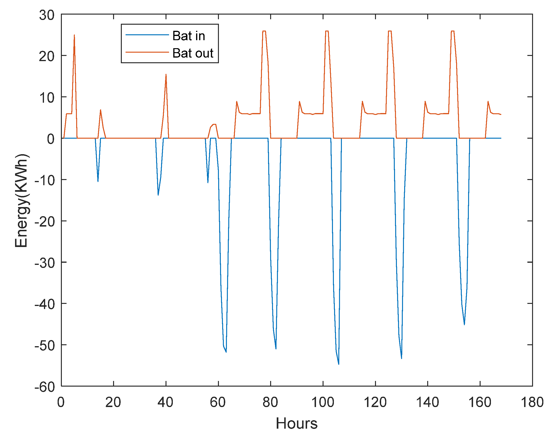
4.3. Microgrid Energy Storage with Fluctuating Renewable Energy

As renewable energy generation such as solar or wind power is inherently variable, energy storage systems such as batteries play a crucial role in ensuring a stable and reliable power supply. In this scenario, the battery is charged during excess renewable energy generation periods, storing energy for later use. When the renewable energy output is insufficient to meet the load demand, the battery discharges to bridge the gap. This ability to balance supply and demand enables the MGs to operate independently and reduce reliance on the traditional grid. By effectively managing energy storage, MGs can enhance the integration of renewable energy sources, improve grid resilience, and contribute to a more sustainable energy future. Figure 17 illustrates the dynamic interplay between energy storage and renewable energy sources in a MG system.

5. Conclusions

This study investigated the design and optimization of a standalone HRES for the ICT center at Adama Science and Technology University. By integrating PV panels, WT, battery banks, and DGs, the system aims to provide a reliable and sustainable power supply. A comprehensive mathematical model simulated the system’s performance while accounting for the stochastic nature of renewable energy sources and the load demand. The optimization problem was formulated as a multi-objective challenge, focusing on minimizing the ASC and LPSP. To tackle this complex problem, we employed an HGA. The simulation results show that the HGA achieved the optimal system configuration, with a LCOE of 0.2546 USD/kWh, an LPSP of 0.58%, and a convergence time of 197.2889 s. These findings demonstrate that the HGA exhibits the fastest convergence time, significantly reducing computational effort compared to both M-GA and M-PSO. Furthermore, the optimization results provide a set of design solutions for the HRES, assisting designers in selecting the most effective configurations. The proposed HRES effectively meets the energy demands of the ICT center, significantly reducing the reliance on fossil fuels and lowering overall energy costs. These findings underscore the potential of HRES in providing reliable and sustainable power for remote and off-grid locations.

Despite the promising outcomes of the proposed method, its data dependency presents a significant limitation. The optimization’s accuracy is critically reliant on the quality and availability of input data, such as solar irradiance, wind speed, and load profiles. Deficiencies in this data can negatively impact both system performance and reliability.

Future research directions may include exploring advanced energy management strategies to further enhance system performance, integrating additional renewable energy sources such as biomass, and assessing the impacts of climate change on system design and operation.

References

1. Fekik, A.; Azar, A.T.; Hameed, I.A.; Hamida, M.L.; Amara, K.; Denoun, H.; Kamal, N.A. Enhancing Photovoltaic Efficiency with the Optimized Steepest Gradient Method and Serial Multi-Cellular Converters. Electronics 2023, 12, 2283. [Google Scholar] [CrossRef]
2. Fekik, A.; Hamida, M.L.; Azar, A.T.; Ghanes, M.; Hakim, A.; Denoun, H.; Hameed, I.A. Robust Power Control for PV and Battery Systems: Integrating Sliding Mode MPPT with Dual Buck Converters. Front. Energy Res. 2024, 12, 1380387. [Google Scholar] [CrossRef]
3. Luna-Rubio, R.; Trejo-Perea, M.; Vargas-Vázquez, D.; Ríos-Moreno, G.J. Optimal Sizing of Renewable Hybrids Energy Systems: A Review of Methodologies. Sol. Energy 2012, 86, 1077–1088. [Google Scholar] [CrossRef]
4. Potrč, S.; Čuček, L.; Martin, M.; Kravanja, Z. Sustainable Renewable Energy Supply Networks Optimization—The Gradual Transition to a Renewable Energy System within the European Union by 2050. Renew. Sustain. Energy Rev. 2021, 146, 111186. [Google Scholar] [CrossRef]
5. Thango, B.A.; Obokoh, L. Techno-Economic Analysis of Hybrid Renewable Energy Systems for Power Interruptions: A Systematic Review. Eng 2024, 5, 2108–2156. [Google Scholar] [CrossRef]
6. Dufo-López, R.; Bernal-Agustín, J.L. Design and Control Strategies of PV-Diesel Systems Using Genetic Algorithms. Solar Energy 2005, 79, 33–46. [Google Scholar] [CrossRef]
7. Al-falahi, M.D.A.; Jayasinghe, S.D.G.; Enshaei, H. A Review on Recent Size Optimization Methodologies for Standalone Solar and Wind Hybrid Renewable Energy System. Energy Convers. Manag. 2017, 143, 252–274. [Google Scholar] [CrossRef]
8. Bashir, N.; Modu, B.; Bahru, J. Techno-Economic Analysis of Off-Grid Renewable Energy Systems for Rural Electrification in North-Eastern Nigeria. Int. J. Renew. Energy Res. 2018, 8, 1217–1228. [Google Scholar]
9. Ajlan, A.; Tan, C.W.; Abdilahi, A.M. Assessment of Environmental and Economic Perspectives for Renewable-Based Hybrid Power System in Yemen. Renew. Sustain. Energy Rev. 2017, 75, 559–570. [Google Scholar] [CrossRef]
10. Sinha, S.; Chandel, S.S. Review of Software Tools for Hybrid Renewable Energy Systems. Renew. Sustain. Energy Rev. 2014, 32, 192–205. [Google Scholar] [CrossRef]
11. Bernal-Agustín, J.L.; Dufo-López, R. Simulation and Optimization of Stand-Alone Hybrid Renewable Energy Systems. Renew. Sustain. Energy Rev. 2009, 13, 2111–2118. [Google Scholar] [CrossRef]
12. Seedahmed, M.M.A.; Ramli, M.A.M.; Bouchekara, H.R.E.H.; Milyani, A.H.; Rawa, M.; Nur Budiman, F.; Firmansyah Muktiadji, R.; Mahboob Ul Hassan, S. Optimal Sizing of Grid-Connected Photovoltaic System for a Large Commercial Load in Saudi Arabia. Alex. Eng. J. 2022, 61, 6523–6540. [Google Scholar] [CrossRef]
13. Tozzi, P.; Jo, J.H. A Comparative Analysis of Renewable Energy Simulation Tools: Performance Simulation Model vs. System Optimization. Renew. Sustain. Energy Rev. 2017, 80, 390–398. [Google Scholar] [CrossRef]
14. Fathy, A.; Kaaniche, K.; Alanazi, T.M. Recent Approach Based Social Spider Optimizer for Optimal Sizing of Hybrid PV/Wind/Battery/Diesel Integrated Microgrid in Aljouf Region. IEEE Access 2020, 8, 57630–57645. [Google Scholar] [CrossRef]
15. Bukar, A.L.; Tan, C.W.; Lau, K.Y. Optimal Sizing of an Autonomous Photovoltaic/Wind/Battery/Diesel Generator Microgrid Using Grasshopper Optimization Algorithm. Sol. Energy 2019, 188, 685–696. [Google Scholar] [CrossRef]
16. Farh, H.M.H.; Al-Shamma’a, A.A.; Al-Shaalan, A.M.; Alkuhayli, A.; Noman, A.M.; Kandil, T. Technical and Economic Evaluation for Off-Grid Hybrid Renewable Energy System Using Novel Bonobo Optimizer. Sustainability 2022, 14, 1533. [Google Scholar] [CrossRef]
17. Mariam, L.; Basu, M.; Conlon, M.F. A Review of Existing Microgrid Architectures. J. Eng. 2013, 2013, 937614. [Google Scholar] [CrossRef]
18. Alegria, E.; Brown, T.; Minear, E.; Lasseter, R.H. CERTS Microgrid Demonstration with Large-Scale Energy Storage and Renewable Generation. IEEE Trans. Smart Grid 2014, 5, 937–943. [Google Scholar] [CrossRef]
19. Lidula, N.W.A.; Rajapakse, A.D. Microgrids Research: A Review of Experimental Microgrids and Test Systems. Renew. Sustain. Energy Rev. 2011, 15, 186–202. [Google Scholar] [CrossRef]
20. Bramm, A.M.; Eroshenko, S.A.; Khalyasmaa, A.I.; Matrenin, P.V. Grey Wolf Optimizer for RES Capacity Factor Maximization at the Placement Planning Stage. Mathematics 2023, 11, 2545. [Google Scholar] [CrossRef]
21. Lei, X. A Photovoltaic Prediction Model with Integrated Attention Mechanism. Mathematics 2024, 12, 2103. [Google Scholar] [CrossRef]
22. Bamisile, O.; Acen, C.; Cai, D.; Huang, Q.; Staffell, I. The environmental factors affecting solar photovoltaic output. Renew. Sustain. Energy Rev. 2025, 208, 115073. [Google Scholar] [CrossRef]
23. Huld, T.; Gottschalg, R.; Beyer, H.G.; Topič, M. Mapping the Performance of PV Modules, Effects of Module Type and Data Averaging. Sol. Energy 2010, 84, 324–338. [Google Scholar] [CrossRef]
24. Skoplaki, E.; Palyvos, J.A. On the Temperature Dependence of Photovoltaic Module Electrical Performance: A Review of Efficiency/Power Correlations. Sol. Energy 2009, 83, 614–624. [Google Scholar] [CrossRef]
25. Ayop, R.; Isa, N.M.; Tan, C.W. Components Sizing of Photovoltaic Stand-Alone System Based on Loss of Power Supply Probability. Renew. Sustain. Energy Rev. 2018, 81, 2731–2743. [Google Scholar] [CrossRef]
26. Fathy, A. Reliable and Efficient Approach for Mitigating the Shading Effect on Photovoltaic Module Based on Modified Artificial Bee Colony Algorithm. Renew. Energy 2015, 81, 78–88. [Google Scholar] [CrossRef]
27. Borhanazad, H.; Mekhilef, S.; Ganapathy, V.G.; Modiri-Delshad, M.; Mirtaheri, A. Optimization of micro-grid system using MOPSO. Renew. Energy 2014, 71, 295–306. [Google Scholar] [CrossRef]
28. Sukamongkol, Y.; Chungpaibulpatana, S.; Ongsakul, W. A Simulation Model for Predicting the Performance of a Solar Photovoltaic System with Alternating Current Loads. Renew. Energy 2002, 27, 237–258. [Google Scholar] [CrossRef]
29. Nadjemi, O.; Nacer, T.; Hamidat, A.; Salhi, H. Optimal Hybrid PV/Wind Energy System Sizing: Application of Cuckoo Search Algorithm for Algerian Dairy Farms. Renew. Sustain. Energy Rev. 2017, 70, 1352–1365. [Google Scholar] [CrossRef]
30. Wang, L.; Tan, A.C.C.; Cholette, M.; Gu, Y. Comparison of the Effectiveness of Analytical Wake Models for Wind Farm with Constant and Variable Hub Heights. Energy Convers. Manag. 2016, 124, 189–202. [Google Scholar] [CrossRef]
31. Justus, C.G. Wind Energy Statistics for Large Arrays of Wind Turbines (New England and Central U.S. Regions). Sol. Energy 1978, 20, 379–386. [Google Scholar] [CrossRef]
32. Bhandari, B.; Lee, K.T.; Lee, G.Y.; Cho, Y.M.; Ahn, S.H. Optimization of Hybrid Renewable Energy Power Systems: A Review. Int. J. Precis. Eng. Manuf. Green Technol. 2015, 2, 99–112. [Google Scholar] [CrossRef]
33. Shin, J.; Lee, J.H.; Realff, M.J. Operational Planning and Optimal Sizing of Microgrid Considering Multi-Scale Wind Uncertainty. Appl. Energy 2017, 195, 616–633. [Google Scholar] [CrossRef]
34. Rehman, S.; Al-Abbadi, N.M. Wind Shear Coefficients and Energy Yield for Dhahran, Saudi Arabia. Renew. Energy 2007, 32, 738–749. [Google Scholar] [CrossRef]
35. Wind Turbines—Part 1: Design Requirements. 2005. Available online: https://dlbargh.ir/mbayat/46.pdf (accessed on 19 April 2024).
36. Kharrich, M.; Kamel, S.; Alghamdi, A.S.; Eid, A.; Mosaad, M.I.; Akherraz, M.; Abdel-Akher, M. Optimal Design of an Isolated Hybrid Microgrid for Enhanced Deployment of Renewable Energy Sources in Saudi Arabia. Sustainability 2021, 13, 4708. [Google Scholar] [CrossRef]
37. Wang, L.; Singh, C. PSO-Based Multi-Criteria Optimum Design of A Grid-Connected Hybrid Power System With Multiple Renewable Sources of Energy. In Proceedings of the IEEE Swarm Intelligence Symposium, Honolulu, HI, USA, 1–5 April 2007. [Google Scholar] [CrossRef]
38. Guangqian, D.; Bekhrad, K.; Azarikhah, P.; Maleki, A. A Hybrid Algorithm Based Optimization on Modeling of Grid Independent Biodiesel-Based Hybrid Solar/Wind Systems. Renew. Energy 2018, 122, 551–560. [Google Scholar] [CrossRef]
39. Skarstein, O.; Uhlen, K. Design Considerations with Respect to Long-Term Diesel Saving in Wind/Diesel Plants. Wind Eng. 1989, 13, 72–87. [Google Scholar]
40. Azoumah, Y.; Yamegueu, D.; Ginies, P.; Coulibaly, Y.; Girard, P. Sustainable Electricity Generation for Rural and Peri-Urban Populations of Sub-Saharan Africa: The “Flexy-Energy” Concept. Energy Policy 2011, 39, 131–141. [Google Scholar] [CrossRef]
41. Mahmoud, M.M.; Ibrik, I.H. Techno-Economic Feasibility of Energy Supply of Remote Villages in Palestine by PV-Systems, Diesel Generators and Electric Grid. Renew. Sustain. Energy Rev. 2006, 10, 128–138. [Google Scholar] [CrossRef]
42. Jayachandran, M.; Ravi, G. Design and Optimization of Hybrid Micro-Grid System. Energy Procedia 2017, 117, 95–103. [Google Scholar] [CrossRef]
43. Zhu, W.; Guo, J.; Zhao, G.; Zeng, B. Optimal Sizing of an Island Hybrid Microgrid Based on Improved Multi-Objective Grey Wolf Optimizer. Processes 2020, 8, 1581. [Google Scholar] [CrossRef]
44. Fathy, A. A Reliable Methodology Based on Mine Blast Optimization Algorithm for Optimal Sizing of Hybrid PV-Wind-FC System for Remote Area in Egypt. Renew. Energy 2016, 95, 367–380. [Google Scholar] [CrossRef]
45. Ndwali, K.; Njiri, J.G.; Wanjiru, E.M. Multi-Objective Optimal Sizing of Grid Connected Photovoltaic Batteryless System Minimizing the Total Life Cycle Cost and the Grid Energy. Renew. Energy 2020, 148, 1256–1265. [Google Scholar] [CrossRef]
46. Bouchekara, H.R.E.H.; Javaid, M.S.; Shaaban, Y.A.; Shahriar, M.S.; Ramli, M.A.M.; Latreche, Y. Decomposition Based Multiobjective Evolutionary Algorithm for PV/Wind/Diesel Hybrid Microgrid System Design Considering Load Uncertainty. Energy Rep. 2021, 7, 52–69. [Google Scholar] [CrossRef]
47. Deb, K.; Pratap, A.; Agarwal, S.; Meyarivan, T. A Fast and Elitist Multiobjective Genetic Algorithm: NSGA-II. IEEE Trans. Evol. Comput. 2002, 6, 182–197. [Google Scholar] [CrossRef]
48. Jin, G.G.; Jarso, A.K. An Improved Hybrid Genetic Algorithm Using the Affine Combination-Based Reproduction. Commun. Stat. Simul. Comput. 2024, 1–27. [Google Scholar] [CrossRef]
49. NASA. NASA POWER Data Access Viewer. 2021. Available online: https://power.larc.nasa.gov/data-access-viewer/ (accessed on 1 January 2021).
Figure 1. Stand-alone microgrid system components and configuration.
Mathematics 13 00985 g001
Figure 2. Characteristic curves of PV array under changing solar irradiance ( G ).
Mathematics 13 00985 g002
Figure 3. WT power output with varying wind speeds.
Mathematics 13 00985 g003
Figure 4. Conceptual framework of proposed rule-based energy management system.
Mathematics 13 00985 g004
Figure 5. NSGA-II procedure.
Mathematics 13 00985 g005
Figure 6. Pareto front of hybrid microgrid optimization problem.
Mathematics 13 00985 g006
Figure 7. Annual wind speed recorded at research site.
Mathematics 13 00985 g007
Figure 8. Annual ambient temperature recorded at research site.
Mathematics 13 00985 g008
Figure 9. Annual solar radiation recorded at research site.
Mathematics 13 00985 g009
Figure 10. Daily load profile of ASTU ICT center.
Mathematics 13 00985 g010
Figure 11. Convergence of objective function value over generations for HGA.
Mathematics 13 00985 g011
Figure 12. Monthly electricity generation from a hybrid system.
Mathematics 13 00985 g012
Figure 13. (a) Generation percentages; (b) ASC percentages.
Mathematics 13 00985 g013
Figure 14. Annualized cost and individual component costs of a microgrid system.
Mathematics 13 00985 g014
Figure 15. Energy contribution of each generating unit over a year: (a) wind; (b) solar; (c) diesel generator; (d) battery.
Mathematics 13 00985 g015
Figure 16. (a) Solar and wind power contribution to load demand; (b) energy balance and battery state of charge (SOC).
Mathematics 13 00985 g016
Figure 17. Battery charging and discharging patterns in hybrid microgrids.
Mathematics 13 00985 g017