Abstract
Previous studies typically assume that output constraints are symmetric or time-invariant. However, effectively addressing asymmetric and time-varying output constraints remains an unsolved issue, especially in the case of switched non-square multi-input multi-output (MIMO) nonlinear systems. To tackle this challenge, this paper first establishes a prescribed-time (PT) Lyapunov criterion for switched nonlinear systems. Second, an asymmetric nonlinear mapping (ANM) method is proposed to handle asymmetric time-varying output constraints. Compared to the barrier Lyapunov function (BLF) approach, the ANM method relaxes the initial output conditions and the constraint functions are not necessarily required to be opposite in sign. Finally, a PT tracking controller is designed for a class of switched MIMO nonlinear systems with a non-square control coefficient matrix by using the time-varying gain technique. This controller achieves zero-error tracking within the prescribed time while ensuring that output constraints are satisfied. The effectiveness of the proposed control strategy is validated through numerical and simulation examples.
Keywords:
switched MIMO nonlinear systems; prescribed-time tracking control; time-varying output constraints; non-square control coefficient matrix MSC:
93-10
1. Introduction
Switched systems, comprising multiple subsystems governed by a deterministic switching law, are extensively utilized to model diverse real-world scenarios, including aircrafts, robotics, and network systems. As a result, the control and stabilization of these systems have garnered significant research interest, as presented in [1,2,3] and related studies. It is worth noting that many practical engineering systems are often modeled by more complex MIMO nonlinear systems, which have been extensively studied in [4,5,6,7]. Furthermore, nonlinear systems with a non-square control coefficient matrix find extensive applications across various engineering domains, including spacecraft attitude control, flexible robotic manipulators, and the swing-up control of gymnastic robots, as illustrated in [8,9,10]. However, control strategies for non-square switched MIMO nonlinear systems remain an open research problem. Therefore, exploring the tracking control problem for non-square switched MIMO nonlinear systems presents a challenging and significant research endeavor.
Recently, an increasing number of researchers are focusing on the finite-time (FT) control of nonlinear systems due to its advantages, such as faster convergence rates and enhanced robustness against disturbances. To achieve FT stability for nonlinear systems, various sophisticated and well-designed methods have been proposed, including the homogeneous approach, backstepping design, dynamic gain control, and adding a power integrator (see [11,12,13,14,15]). It is worth noting that the estimation of settling time in FT control heavily depends on initial conditions. To address this limitation, the concept of fixed-time (FxT) stability was introduced (see [16,17,18,19]). FxT stability is notable for its ability to estimate an upper bound of settling time that is independent of initial conditions. However, while FxT stability provides advantages in settling time estimation, the relationship between control parameters and the upper bound of the settling time is often complex, and the settling time is frequently overestimated. As a result, the concept of prescribed-time (PT) stability has been introduced, allowing users to arbitrarily specify the system’s convergence time based on practical requirements, regardless of the initial conditions. Specifically, PT stability has been successfully applied to various complex control problems, including uncertain nonlinear systems with time delays in [20]. Due to its distinct advantages, PT stability has garnered significant research interest in the control community (see [21,22,23]).
On the other hand, many real-world systems are often required to satisfy specific output constraints. As a result, the control of nonlinear systems with output constraints has attracted significant attention, as highlighted in studies such as [24,25,26,27]. The BLF has proven to be an effective tool for both controller design and stability analysis in such systems. As the system state variable approaches the predefined constraint boundary, the BLF value tends to infinity. Ensuring the boundedness of the BLF can effectively prevent constraint violations. However, as noted in [28], control algorithms based on BLFs often require transforming the output constraint problem into a tracking error constraint problem, which results in more conservative initial output conditions. By introducing a nonlinear transformation that is dependent on the output, the authors of [28] proposed an adaptive control method for single-input single-output systems with time-varying output constraints, which relaxes the initial output condition requirements. Nevertheless, this approach does not account for switching or MIMO characteristic in the modeling. Additionally, the time-varying output constraints considered in [28] are not arbitrary functions but must satisfy specific conditions. For instance, the output is required to satisfy , where and are assumed to be positive functions.
Motivated by these observations, we now formulate the following research question:
For switched MIMO systems with time-varying output constraints and non-square control coefficient matrices, how can we achieve prescribed-time trajectory tracking control?
In this paper, we aim to provide a comprehensive answer to this question. The contributions of this work are listed in the following three aspects:
- (1)
- The conservatism in initial conditions inherent to BLF-based control methods, as observed in [24,25,26,27], poses significant challenges for practical implementation. Although the integral BLF approach proposed in [29] alleviates this issue to some extent, it remains ineffective in addressing time-varying asymmetric output constraints. To address this limitation, we employ the ANM method, effectively alleviating the conservatism in the system’s initial output constraints.
- (2)
- The proposed ANM method is applicable to asymmetric time-varying output constraints, including unilateral constraints, unconstrained cases, and constant constraints, offering greater generality compared to the nonlinear transferred function approach discussed in [28]. Our approach permits the constraint functions to be arbitrary smooth time-varying functions, in contrast to [27,28,30], where they are required to have opposite signs.
- (3)
- Compared to the MIMO systems with square coefficient matrices studied in [4,5,6], this work proposes a unified design approach that is applicable not only to square MIMO systems but also effectively handles non-square MIMO systems, achieving zero-error tracking within a prescribed time.
The rest of this paper is organized as follows. Section 2 presents the system model and preliminaries. Section 3 details the proposed control strategy and conducts an in-depth stability analysis. Section 4 presents numerical and simulation examples with corresponding results to validate the theoretical findings. The paper concludes with some remarks in Section 5.
2. Problem Formulation
2.1. System and Assumptions
This work investigates the following switched MIMO system:
where , , , and () are the state and control input vectors, respectively. Differently from the switching mechanism in [31], where the switching is governed by a stochastic Markov process, our switching signal, denoted as , is a deterministic, piecewise constant and right continuous function. Throughout this paper, we assume that all the states of (1) remain continuous at each switching instant, and there is a finite number of switchings for the switching signal within any finite time interval. For any , the matrix denotes the control coefficient matrix, which is not necessarily symmetric, and the function consists of unknown smooth nonlinear vectors, which represents non-vanishing disturbance.
Let us denote and as the constraint function vectors. The objective of this paper is to design a tracking controller that ensures that all state variables remain bounded, while enabling the output to accurately track a reference signal within any prescribed time without violating the predetermined output constraint
Remark 1.
We emphasize that the constraint functions and , can be any smooth time-varying functions. This distinguishes our approach from the requirement in [27,28,30], where the two constraint functions must have opposite signs. In practical applications, output constraint functions may both be positive, both negative, or differ in sign. Our method offers a more general and flexible framework, broadening its applicability to a wider range of constrained control problems.
Assumption 1.
For any , there exist the unknown bounded function and the known smooth function such that
where is bounded by an unknown constant .
Assumption 2.
For any , the control coefficient matrix can be decomposed as
where is a known matrix, with , for , being nonzero vectors, and is a square matrix that is not necessarily symmetric. Moreover, the matrix is symmetric and positive-definite, i.e.,
where is a known constant and denotes the minimum eigenvalue of the matrix •.
Assumption 3.
For any , there exist the constants such that the time-varying functions and their time derivative satisfy
where denote the first-order time derivatives of and , respectively, i.e., and .
Assumption 4.
For any , there exist the known time-varying functions and positive constants , , such that the desired trajectory satisfies and its i-th time derivatives satisfy ,
Remark 2.
Assumption 2 is introduced to address the non-invertibility issue of non-square coefficient matrices. The non-square nature of the system introduces significant challenges in controller design, as illustrated in inequality (37). Assumption 2 provides the necessary theoretical foundation for achieving prescribed-time tracking control. It is worth noting that similar conditions have been successfully applied in [9,32]. Moreover, this assumption effectively characterizes various practical engineering systems, including spacecraft attitude control, flexible robotic manipulators, and the swing-up control of gymnastic robots, with relevant applications discussed in [8,9,10].
2.2. Preliminaries
In this paper, and denote the set of nonnegative real numbers and the real n-dimensional space, respectively. For a given matrix A, denotes its transpose. For a given vector X, is the Euclidean norm. Define for a matrix . Let denote all nonnegative functions on , which are continuously differentiable in t and twice continuously differentiable in .
We introduce the following scaling function:
where is an integer and is a freely prescribed time. Obviously, is a monotonically increasing function on with and . Meanwhile, is continuously differentiable with respect to t and
In the following part, we introduce two lemmas, which are useful for our subsequent controller design and stability analysis.
Theorem 1.
Consider a switched nonlinear system with being defined as that in (1) and being a smooth function. If there exist a non-negative function and the positive constants , such that for all , ,
then the function satisfies
Proof.
Let be the switching time instants of the switching signal in system (19). During the time interval (), the -th subsystem is activated. Then, there exists a time interval such that . For any , from (6) and (8), we have
which implies that
We compute the term on the left side of (11) to obtain
On the right-hand side of (11), it can be derived that
Based on (12) and (13), we have
This completes the proof of Theorem 1. □
3. Control Design and Stability Analysis
3.1. State-Constrained Transformation
Let us define the tracking error , where for . In light of the output constraint (2), it can be verified that () must satisfy the constraint condition:
To tackle the issue of output constraint (15),we introduce the following asymmetric nonlinear mapping (ANM):
where is an indicator function defined by
The aforementioned transformation is well-defined on the condition that the error variables , adhere to the constraint condition (15). Consequently, if is satisfied, then the variables , will indeed comply with the constraint condition (15). In fact, the ANM method is designed to transform the output-constrained problem into a bounded tracking error problem by introducing a nonlinear mapping function (15). We see that the output constraints will not be violated as long as is bounded. Moreover, according to Assumptions 3 and 4, we know that both and are positive and bounded, i.e., there exist positive constants and such that and . Thus, if , satisfies (15), then it follows from (16) that
Noting that for , we further know that holds for all . In addition, it can be inferred that is continuously differentiable with respect to its arguments and
It is easy to compute that
Due to the fact that
we can obtain
Using the transformation (16), together with the switched MIMO system (1), yields
where , and are defined by , , with , .
Remark 3.
Compared with the existing results, such as [24,25], the ANM method offers a broader range of applicability and can be categorized into the following cases:
Case 1 [Symmetric time-varying constraints, i.e., and , ]. Under the assumption of symmetric and time-varying output constraints, the ANM (16) still works with
Case 2 [Symmetric constant constraints, i.e., and , ]. In this case, the output constraints are assumed to be positive numbers. Then, the system (1) degenerates into the case studied in [24,25]. Response: The underline is necessary to clearly present the classification and should be retained in all highlighted parts.
Case 3 [Unilateral constraints or non-constraints, i.e., or , ]. In the unilateral constraint case, the output variable is required to be or for all . Taking the first case as an example, the ANM (16) is changed into
On the other hand, our results can be extended to the case where no constraints are imposed on the output . In this case, the ANM (16) can reduce into a trivial transformation , .
3.2. Controller Design
Let us define
where are the virtual controllers to be specified later. In the following, we focus on the control design of the switched MIMO system (1). The design process is carried out by using the backstepping methodology.
Step 1. Let us consider a candidate Lyapunov function . Then, the dynamics of , , are
Combining with (19) yields
For any , in accordance with Assumptions 3 and 4, there exist the positive constants and such that and . It is noteworthy that the relationship holds true for . Therefore, by using the fact for and Young’s inequality, we can derive
where . Similarly,
where . Denote , , and . Obviously, the matrix is invertible due to the positiveness of , . It follows from (23)–(25) that
where . Due to the fact that , the last term in the above equation can be rewritten as . Noting that for , we have . By taking
with being a real number, then it follows that
Hence, we know from (26) that .
Step 2. Let us consider a candidate Lyapunov function . The dynamic of is
Then, along with the solution of (29), it follows that
Note that . By using the Young inequality, we have
By taking
with being a real number, we have .
Repeating this step, we can obtain the dynamic of
and find a () in the form of
with being a real number, such that
where , , and are positive real numbers.
Stepn. Consider a Lyapunov function . The dynamic of is
Then, along with the solution of (35), it follows that
By using the Young inequality, we have
where , is a control parameter. Note, that
Hence, by taking
with being a real number, we have
Therefore, we obtain
where and are positive constants.
Remark 4.
Since in system (1) is not necessarily a square matrix, directly applying the inverse of for controller design, as in [5,6,24], is unfeasible. To address this, we decompose into a non-square matrix and a square matrix , as stated in Assumption 2. This enables controller design even when is non-invertible. However, since is unknown and cannot be directly utilized, constructing a control input based on is challenging. To resolve this, we incorporate inequality (37) and design a prescribed-time tracking controller relying solely on , eliminating the dependence on and ensuring convergence within the prescribed time.
3.3. Stability Analysis
Theorem 2.
Under Assumptions 1–4, there exists a tracking controller u in the form of (38) for system (1) such that for any initial data satisfying , ,
- (1)
- the prescribed output constraint is not violated, i.e., the output satisfies
- (2)
- all signals of the closed-loop system are bounded on ;
- (3)
- the tracking error possesses the following property:where represents the first time derivative of .
Proof.
(1) According to Theorem 1 and (39), we know that remains bounded over the interval . This, in turn, implies that the variables , , are also bounded within the same interval. Observing (21), we deduce that , are also bounded, as . Consequently, by referring to (16), we can assert that , hold for all . Given the relationship , , we can further obtain
Considering the definitions of and in (15), we conclude that the output will obey the pre-assigned output constraint provided that the initial value satisfies .
(2) Based on (21) and (39), we know that and , , are bounded over the interval . Moreover, combining with , , it can be inferred that .
Next, we need to show the boundedness of the controller u. First, we consider the boundedness of the first virtual controller . Based on Assumption 4, it follows that is bounded. Noting that , we have . Considering that and are both bounded on the interval , we conclude that the virtual controller is bounded on .
Second, we consider the boundedness of the second virtual controller . Recall that
For any , according to the definition of and the boundedness of and , we have
Given that , are bounded, and , it is sufficient to ensure that remains bounded, provided that is also bounded. Let us denote . Based on the definition of , we can derive that
Denote . For any , it follows from (22) and (27) that
Note, that
and . Hence, due to the fact that , we have
Since is bounded over the interval , we know that there exists a finite constant such that
Applying the L’Hôpital’s rule, we have
Combining with (46) and applying the L’Hôpital’s rule again yields
Case 1 For , it follows from (49) that , which indicates that is bounded on the interval . Moreover, it further follows that tends to zero at a rate not slower than . Thus, we know that tends to zero at a rate not slower than as t approaches . Thus, we can ensure the boundedness of on according to (44).
Case 2 For , we can deduce from (49) that tends to zero at a rate not slower than and tends to zero at a rate not slower than as t approaches . Therefore, in conjunction with (44), we can conclude that is bounded over the interval .
Consequently, the boundedness of can be guaranteed over the interval , which in turn implies that is also bounded.
By repeatedly applying the L’Hôpital’s rule to (49), we establish that , for and , approaches zero at a rate of no less than as t nears . By analogous reasoning applied to (44)–(46), we can similarly demonstrate that , , also tends to zero at a comparable rate as t approaches . Consequently, it is sufficient to show that , for and , remains bounded over the interval . Observing that , , we deduce that , is bounded. In conjunction with (38), we can conclude that u is bounded on the interval .
Remark 5.
As noted in [28], the BLF method often requires the initial output to be restricted within a smaller range than the actual constraints, whereas the ANM method effectively avoids this limitation. To illustrate this issue, we consider the following system with output constrained by a constant bound:
where , is the control input, and are the system states. The system output y is subject to the following constraint: , where is a known positive constant. Define the tracking error as , where is a known reference signal. We consider the following logarithmic BLF:
where , , Y is a positive constant. The BLF approach guarantees compliance with the output constraint by restricting the tracking error within the bound: . Recalling the definition of , we obtain . When , which implies that:
Since , it follows that , leading to a more restrictive initial range for the output signal than the original constraint . Thus, by adopting the ANM method, we effectively circumvent the conservativeness associated with the BLF-based control algorithm regarding the initial value of the system output.
Remark 6.
It is noteworthy that this work centers on achieving PT tracking control, a goal that diverges from the findings presented in [4,7,9,22]. The pivotal difference resides in our employment of the ANM method to address output constraints, thereby recasting the output-constrained challenge into an investigation of the boundedness of , . Conversely, by using the time-varying gain technique and L’Hôpital’s rule, a zero-error tracking outcome is attainable. For analogous results, refer to [7], where a full-state tracking result is obtained for normal MIMO systems. Indeed, due to the presence of output constraints and the ANM (16), a nonlinear term is incorporated into (19). It can be easily verified that this nonlinear term vanishes as , approaches zero. Consequently, a good tracking result, , is ensured. Given that numerous physical systems can be represented as two-dimensional nonlinear systems, this tracking outcome is adequately sufficient for a broad spectrum of practical applications.
4. Example
In this section, two examples are provided to validate our theoretical results.
Example 1.
Consider the following three-dimensional switched MIMO system:
where ,, and are the state and control input vectors, respectively. The switching signal takes values from the set . The system parameters are defined as follows:
Consider the output variable , which is required to satisfy the time-varying constraints for all . The time-varying constraint function vectors are defined as:
Furthermore, the reference trajectories are given by
Besides, it can be verified that Assumption 1 holds by choosing . By choosing the matrix
it can be verified that Assumption 2 holds, and the minimum eigenvalue satisfies . Clearly, Assumption 3 is satisfied with , .
Based on the control framework introduced in Section 3, we design a tracking controller as follows:
where , and are defined in (21) with . For the simulation, the initial condition is given as , , and the design parameters are set as , , , , and .
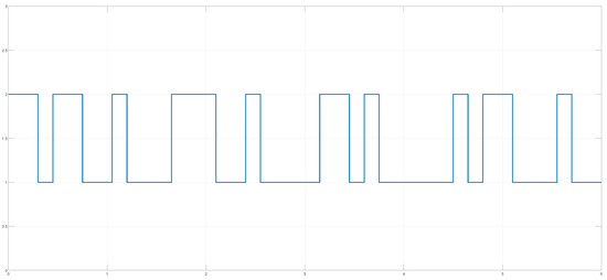
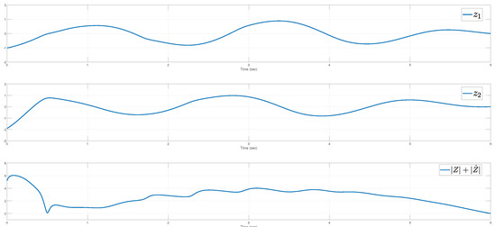
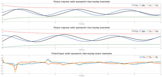
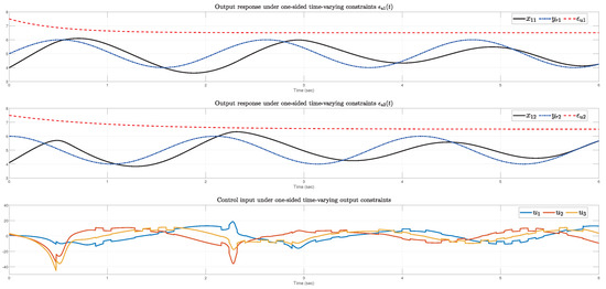
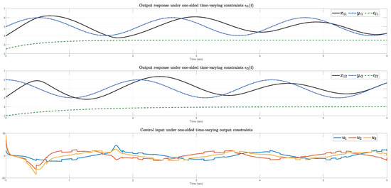
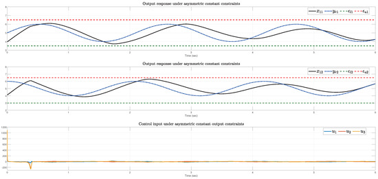
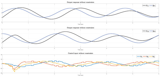
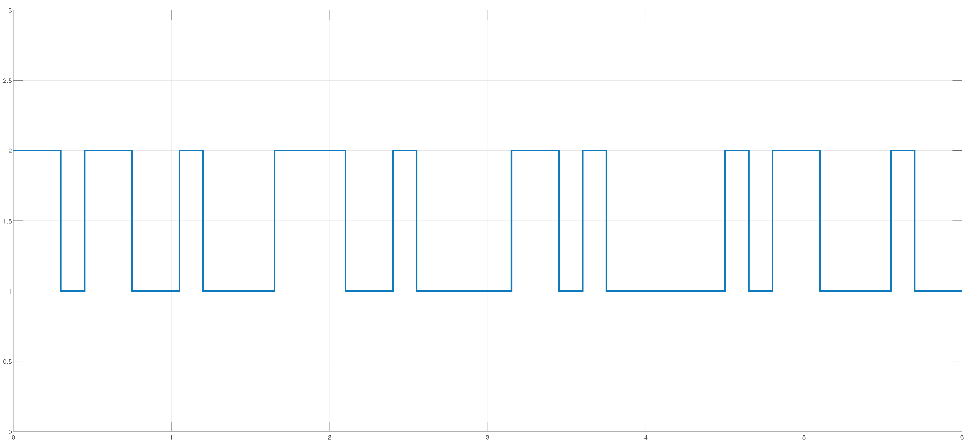
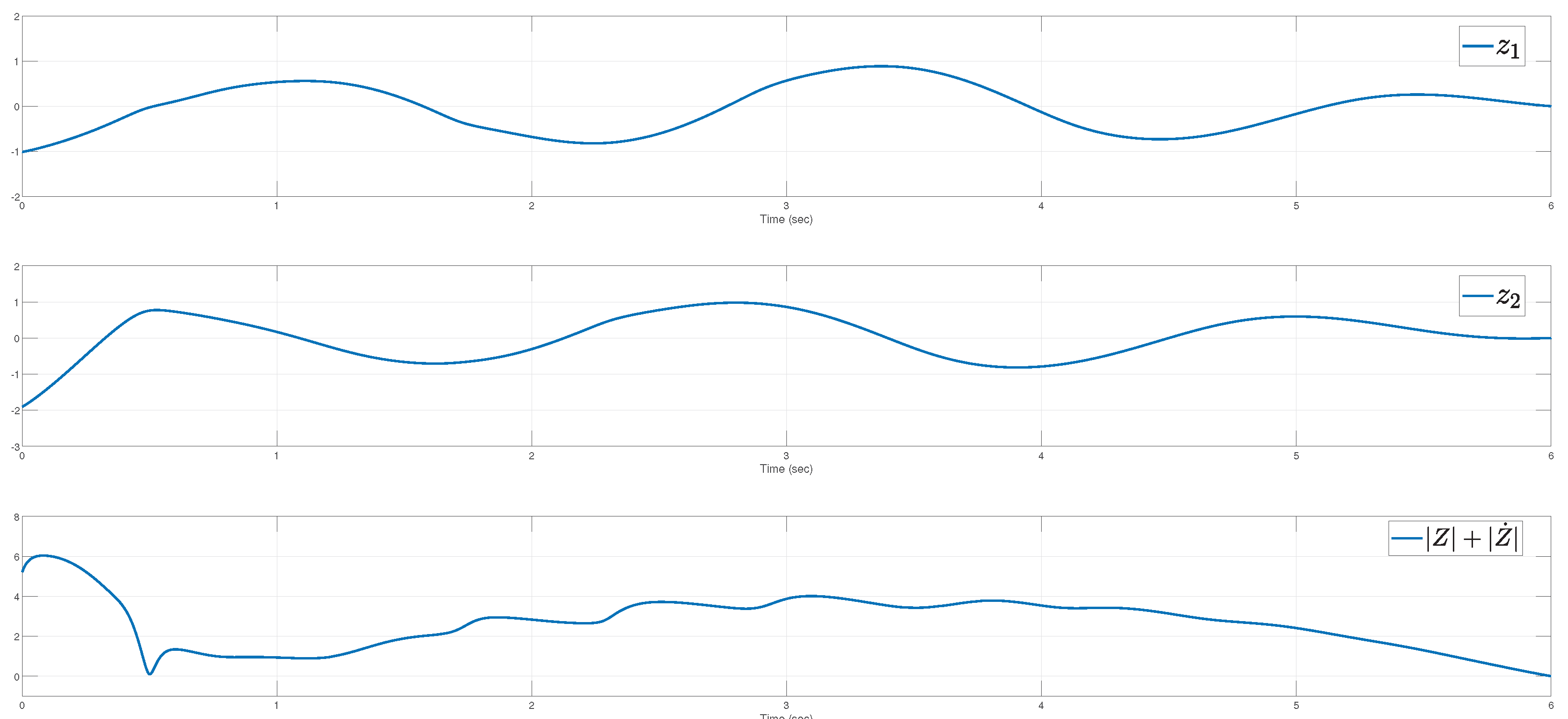
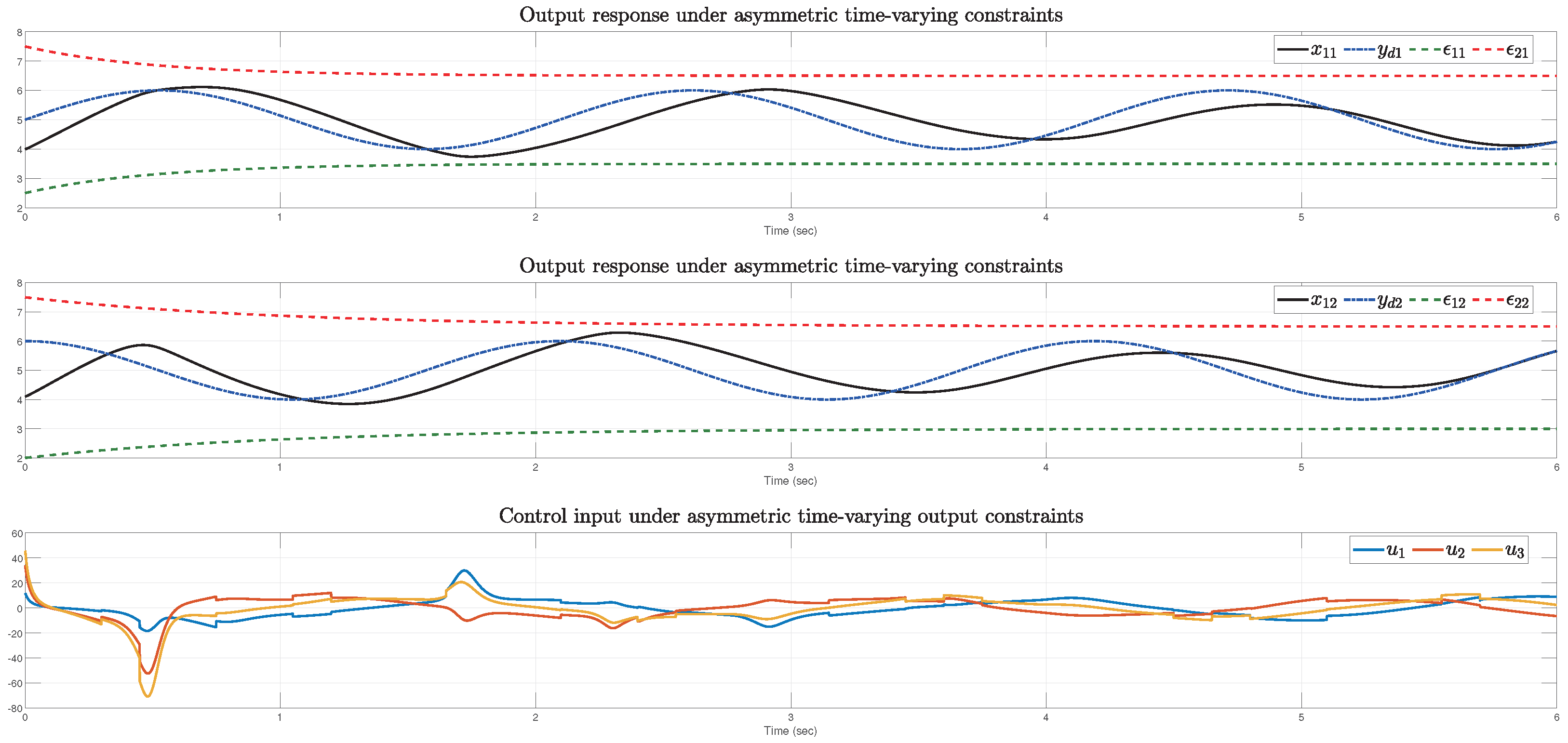
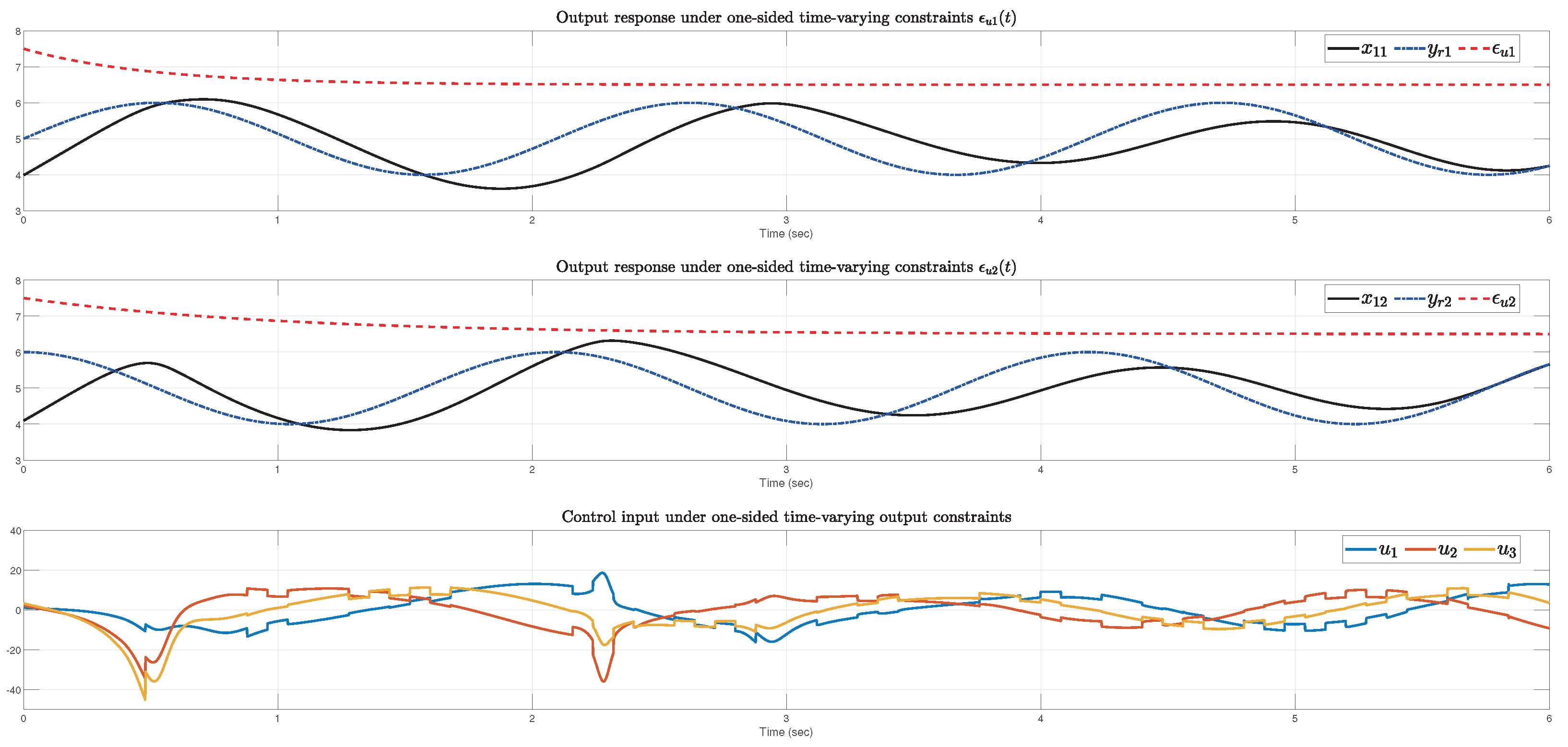
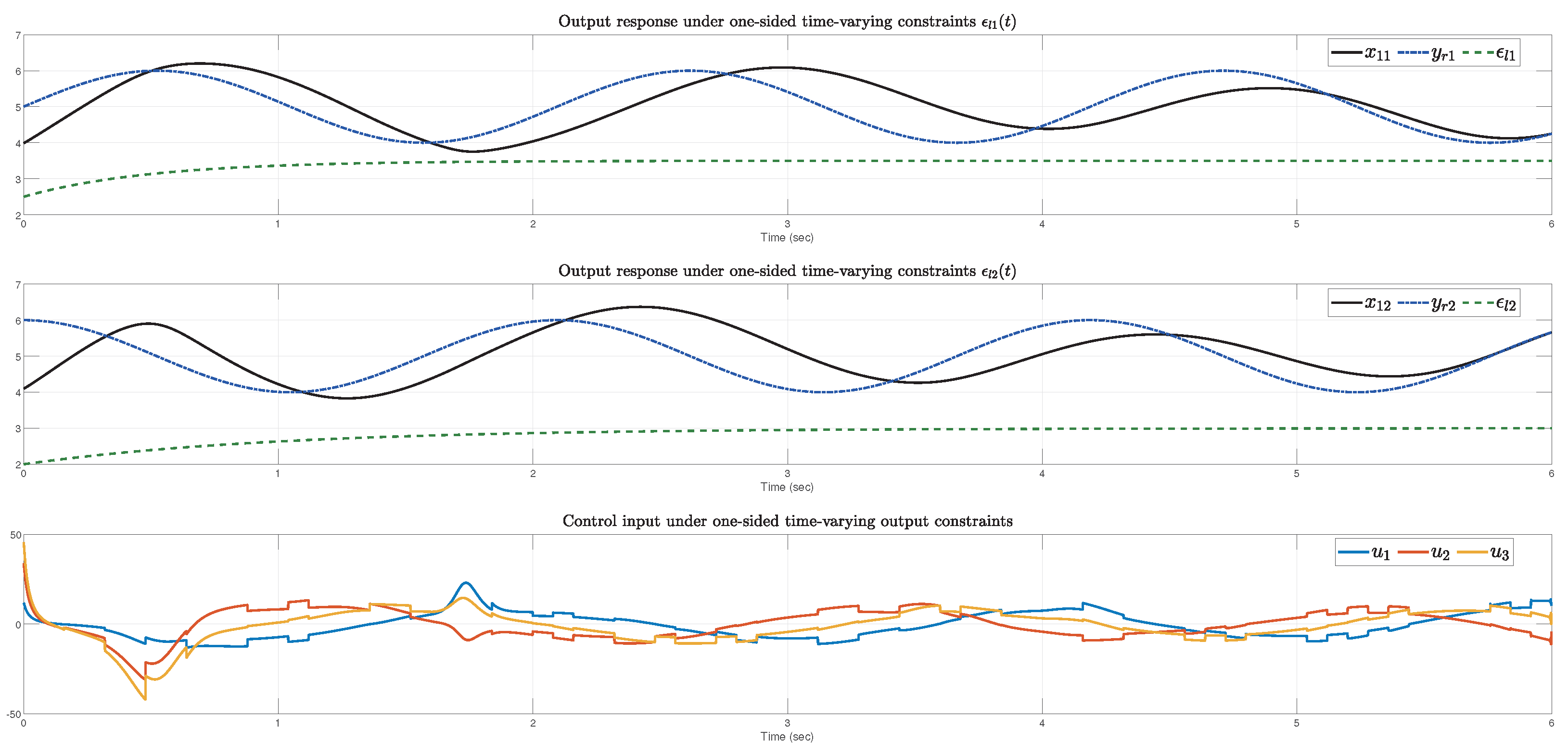
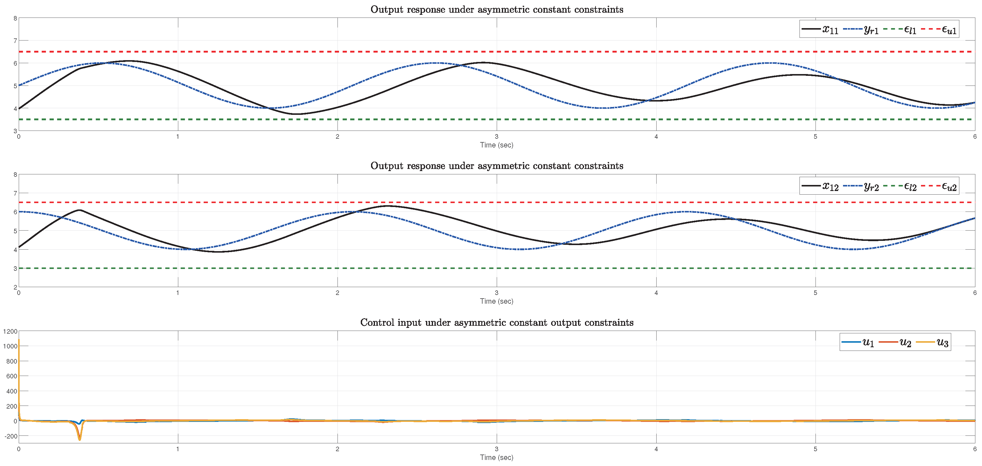
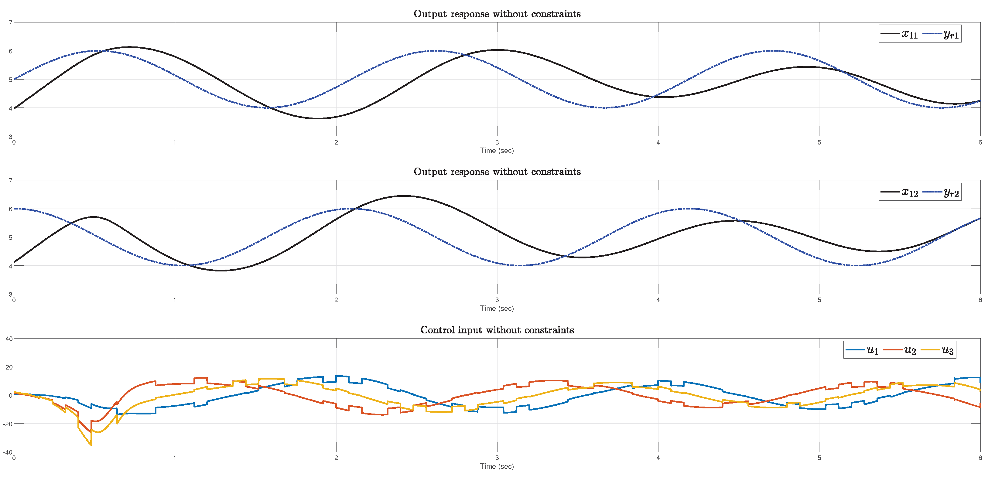
The simulation results are given in Figure 1, Figure 2, Figure 3, Figure 4, Figure 5, Figure 6 and Figure 7. Figure 2 illustrates that the output tracking errors converge to zero at the prescribed time, while the norm of the derivative of the tracking error also converges to zero. Figure 3 demonstrates that the time-varying asymmetric output constraints are strictly satisfied, and the control signal u remains bounded. To better illustrate the advantages of the ANM method, we present the control performance and output tracking under different constraint settings (see Figure 4, Figure 5, Figure 6 and Figure 7), including unilateral constraints, constant constraints, and the unconstrained case. This confirms that the ANM method is applicable to all these scenarios, as stated in Remark 3. Compared to the unconstrained case, the control input u exhibits greater variation under time-varying asymmetric output constraints. This is because the system must exert more control effort to ensure that the state remains within the prescribed constraint boundaries.
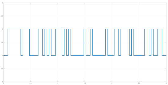
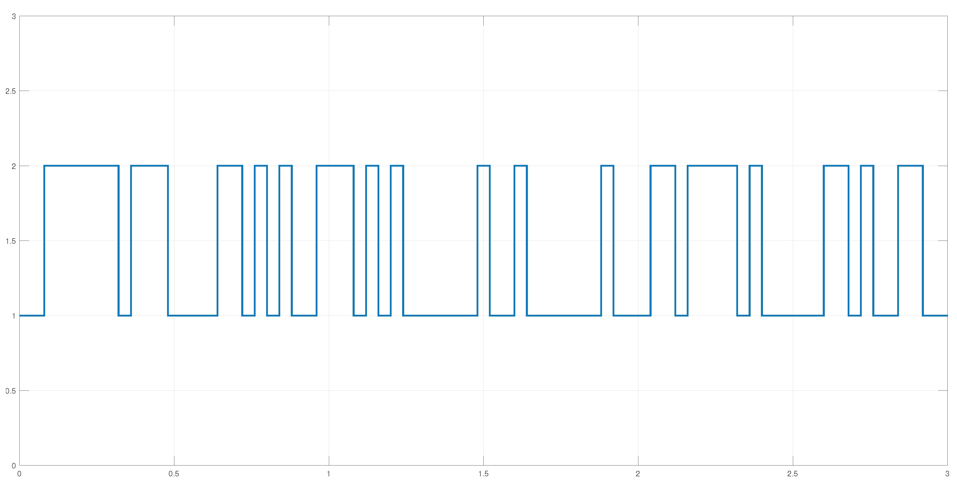
Figure 1.
The switching law in Example 1.
Figure 2.
The output tracking error in Example 1.
Figure 3.
Output and control input under asymmetric time-varying constraints in Example 1.
Figure 4.
Output and control input under one-sided time-varying constraints in Example 1.
Figure 5.
Output and control input under one-sided time-varying constraints in Example 1.
Figure 6.
Output and control input under asymmetric constant constraints in Example 1.
Figure 7.
Unconstrained output and control input in Example 1.
Example 2.
Consider a spacecraft system driven by four reaction wheels as mentioned in [8], where the nonlinear dynamics of the system are given by
where represents the attitude angles of the spacecraft, represents the angular velocity of the spacecraft, and represents the control torques imposed on the four reaction wheels. is an extended inertia matrix with being the inertia matrix, and represents the nonlinear disturbance term with being a skew-symmetric matrix of defined by
In this example, switching dynamics are incorporated into system modeling to capture the variation in outer surroundings, i.e., represents the switching signal taking values from the set . We select the matrices in the above model as
Assume that the output variable , and must fulfill () for all . The time-varying constraint function vectors and are set as
The desired trajectories of attitude angles are chosen as
It is easy to show that , with being some unknown disturbance and (which is computable and not unique). Hence, it shows that Assumption 1 holds. Based on (58), it can be computed that the matrix is setting as
which implies that Assumption 2 holds with . According to (2), Assumption 3 is satisfied with , .
Based on the control framework introduced in Section 3, we design a tracking controller as follows:
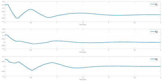
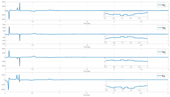
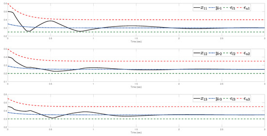
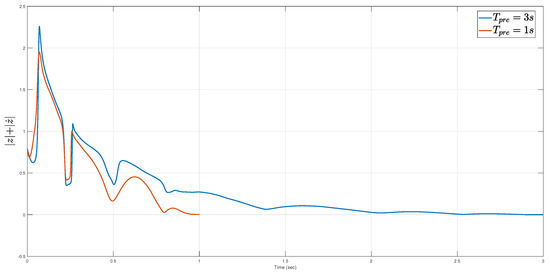
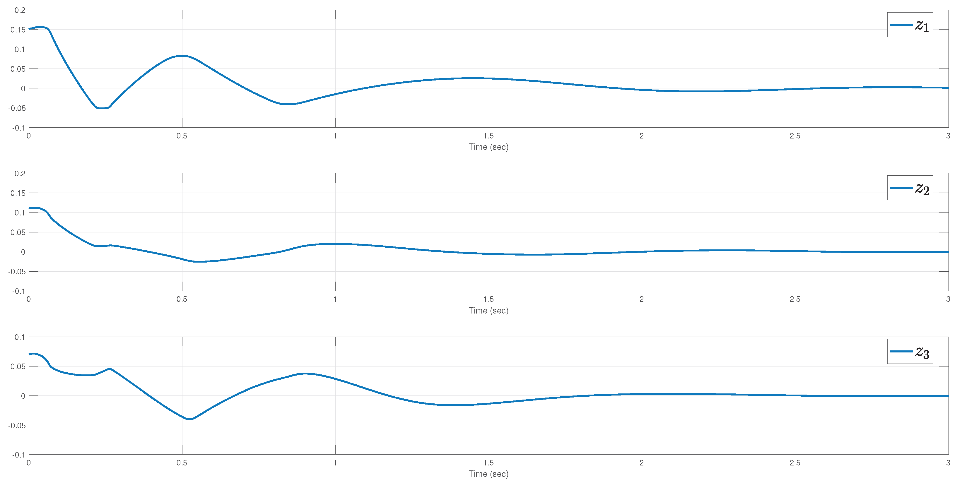
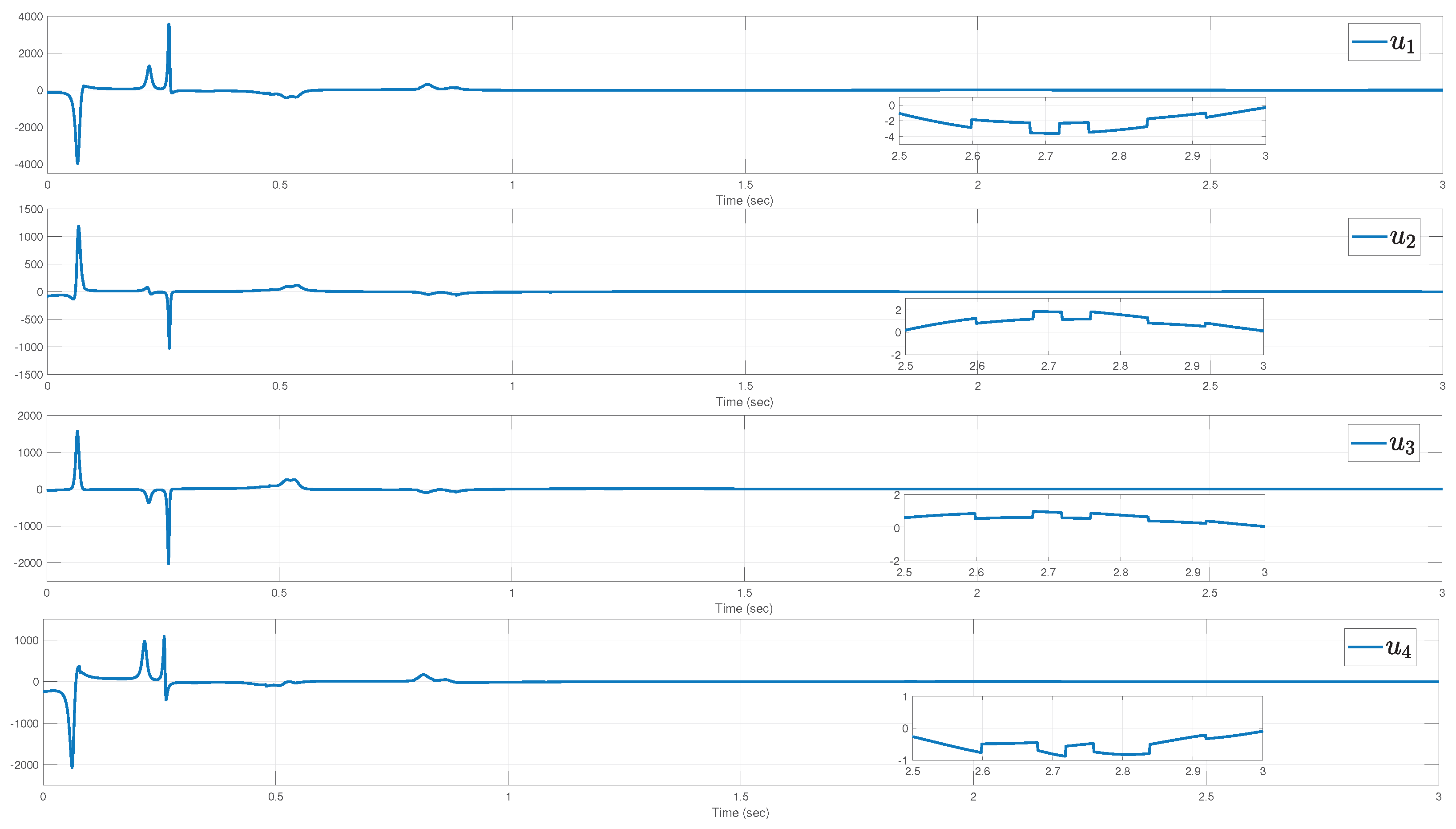
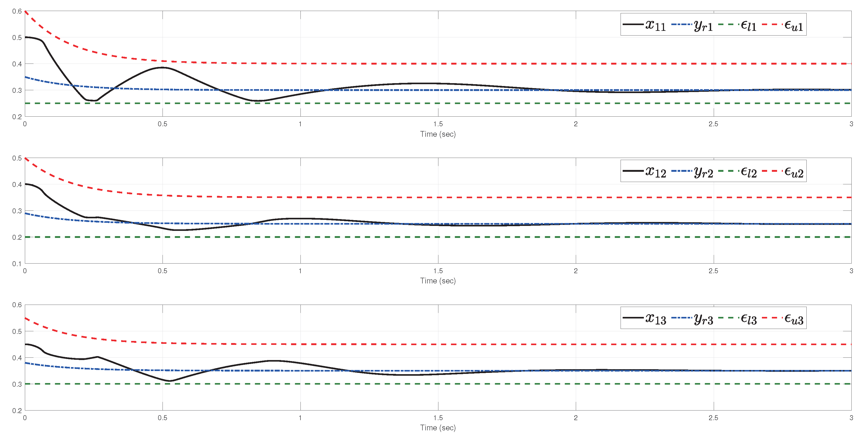
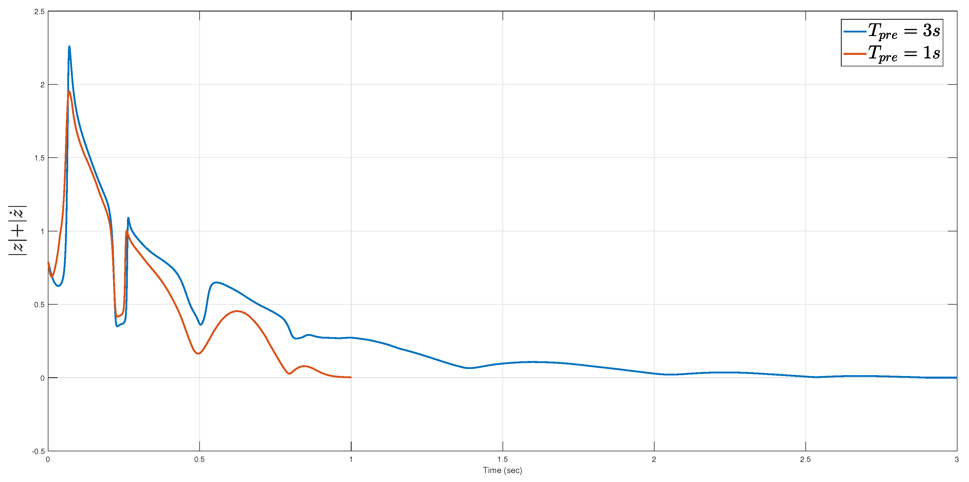
where , and are defined in (21) with . For the simulation, the initial condition is given as , , and the design parameters are set as , , , and . The simulation results are given in Figure 8, Figure 9, Figure 10, Figure 11 and Figure 12. Figure 9 shows that the output tracking errors () converge to zero at the prescribed time, verifying the effectiveness of the proposed control strategy in achieving zero-error trajectory tracking. Figure 10 illustrates that the control input u remains bounded throughout the tracking process. From Figure 11, we can infer that the time-varying asymmetric output constraints are satisfied, confirming that the ANM approach successfully prevents constraint violations. Figure 12 presents the variation of the tracking error under different prescribed times, further validating the flexibility of the proposed method in achieving prescribed-time convergence with different time settings.
Figure 8.
The switching law in Example 2.
Figure 9.
The output tracking error in Example 2.
Figure 10.
The control input in Example 2.
Figure 11.
The output response under asymmetric time-varying constraints in Example 2.
Figure 12.
Comparison of tracking error under different prescribed times in Example 2.
Remark 7.
Although the boundedness of all signals has been theoretically proven, numerical simulations often encounter issues due to the unbounded nature of the time-varying gain as t approaches . To circumvent this problem and enable practical simulation, we introduce a small positive parameter to modify , resulting in . This method is consistent with the techniques employed in [33,34].
5. Conclusions
A PT tracking control method is proposed for a class of switched MIMO nonlinear systems with asymmetric time-varying output constraints. By combining the tangent-type ANM and the backstepping recursive design strategy, the proposed controller effectively achieves zero-error tracking while ensuring that all closed-loop signals remain bounded and satisfy the specified output constraints. Simulation results confirm that the method successfully achieves the desired tracking performance. In future work, we will investigate prescribed-time tracking control for switched stochastic MIMO systems, considering both system uncertainties and external disturbances. Furthermore, we will develop an adaptive controller based on the backstepping method to achieve prescribed-time tracking control.
Author Contributions
Conceptualization, Y.L. and H.W.; methodology, Y.L. and H.W.; software, F.J.; validation, H.W. and Q.Z.; formal analysis, H.W. and Q.Z.; investigation, F.J.; resources, F.J.; data curation, Y.L. and H.W.; writing—original draft preparation, Y.L.; writing—review and editing, Y.L. and H.W.; supervision, Q.Z.; project administration, Q.Z.; funding acquisition, Q.Z. All authors have read and agreed to the published version of the manuscript.
Funding
This research was funded by the National Natural Science Foundation of China, grant numbers 62003170 and 62303001.
Data Availability Statement
The data that support the findings of this study are available from authors upon reasonable request.
Conflicts of Interest
The authors declare no conflicts of interest.
References
- Li, S.; Ahn, C.K.; Guo, J.; Xiang, Z.R. Global output feedback sampled-data stabilization of a class of switched nonlinear systems in the p-normal form. IEEE Trans. Syst. Man Cybern. Syst. 2019, 51, 1075–1084. [Google Scholar] [CrossRef]
- Liberzon, D. Finite data-rate feedback stabilization of switched and hybrid linear systems. Automatica 2014, 50, 409–420. [Google Scholar] [CrossRef]
- Pavlichkov, S.S.; Dashkovskiy, S.N.; Pang, C.K. Uniform stabilization of nonlinear systems with arbitrary switchings and dynamic uncertainties. IEEE Trans. Autom. Control 2016, 62, 2207–2222. [Google Scholar] [CrossRef]
- Kong, L.H.; He, W.; Liu, Z.J.; Yu, X.B.; Silvestre, C. Adaptive tracking control with global performance for output-constrained MIMO nonlinear systems. IEEE Trans. Autom. Control 2022, 68, 3760–3767. [Google Scholar] [CrossRef]
- Liu, Y.C.; Zhu, Q.D. Adaptive neural network asymptotic control design for MIMO nonlinear systems based on event-triggered mechanism. Inf. Sci. 2022, 603, 91–105. [Google Scholar] [CrossRef]
- Xu, H.; Yu, D.; Sui, S.; Zhao, Y.P.; Chen, C.L.P.; Wang, Z. Nonsingular practical fixed-time adaptive output feedback control of MIMO nonlinear systems. IEEE Trans. Neural Netw. Learn. Syst. 2022, 34, 7222–7234. [Google Scholar] [CrossRef]
- Ye, H.F.; Song, Y.D. Prescribed-time tracking control of MIMO nonlinear systems with nonvanishing uncertainties. IEEE Trans. Autom. Control 2022, 68, 3664–3671. [Google Scholar] [CrossRef]
- Shao, X.D.; Hu, Q.L.; Shi, Y.; Zhang, Y.M. Fault-tolerant control for full-state error constrained attitude tracking of uncertain spacecraft. Automatica 2023, 151, 110907. [Google Scholar] [CrossRef]
- Song, Y.D.; Huang, X.C.; Wen, C.Y. Tracking control for a class of unknown non-square MIMO nonaffine systems: A deep-rooted information based robust adaptive approach. IEEE Trans. Autom. Control 2015, 61, 3227–3233. [Google Scholar] [CrossRef]
- Xin, X.; Kaneda, M. Swing-up control for a 3-DOF gymnastic robot with passive first joint: Design and analysis. IEEE Trans. Robot. 2007, 23, 1277–1285. [Google Scholar] [CrossRef]
- Levant, A. Homogeneity approach to high-order sliding mode design. Automatica 2005, 41, 823–830. [Google Scholar] [CrossRef]
- Du, H.B.; Qian, C.J.; Yang, S.Z.; Li, S.H. Recursive design of finite-time convergent observers for a class of time-varying nonlinear systems. Automatica 2013, 49, 601–609. [Google Scholar] [CrossRef]
- Zhang, X.F.; Feng, G.; Sun, Y.H. Finite-time stabilization by state feedback control for a class of time-varying nonlinear systems. Automatica 2012, 48, 499–504. [Google Scholar] [CrossRef]
- Hong, Y.G.; Wang, J.K.; Cheng, D.Z. Adaptive finite-time control of nonlinear systems with parametric uncertainty. IEEE Trans. Autom. Control 2006, 51, 858–862. [Google Scholar] [CrossRef]
- Song, X.N.; Wu, C.L.; Song, S.; Stojanovic, V.; Tejado, I. Fuzzy wavelet neural adaptive finite-time self-triggered fault-tolerant control for a quadrotor unmanned aerial vehicle with scheduled performance. Eng. Appl. Artif. Intell. 2024, 131, 107832. [Google Scholar] [CrossRef]
- Polyakov, A. Nonlinear feedback design for fixed-time stabilization of linear control systems. IEEE Trans. Autom. Control 2011, 57, 2106–2110. [Google Scholar] [CrossRef]
- Polyakov, A.; Efimov, D.; Perruquetti, W. Finite-time and fixed-time stabilization: Implicit Lyapunov function approach. Automatica 2015, 51, 332–340. [Google Scholar] [CrossRef]
- Ning, B.D.; Han, Q.L.; Zuo, Z.Y.; Ding, L.; Lu, Q.; Ge, X.H. Fixed-time and prescribed-time consensus control of multi-agent systems and its applications: A survey of recent trends and methodologies. IEEE Trans. Ind. Inform. 2022, 19, 1121–1135. [Google Scholar] [CrossRef]
- Chen, C.C.; Sun, Z.Y. Fixed-time stabilisation for a class of high-order non-linear systems. IET Control Theory Appl. 2018, 12, 2578–2587. [Google Scholar] [CrossRef]
- Zhang, Z.X.; Zhang, K.; Xie, X.P.; Stojanovic, V. ADP-based prescribed-time control for nonlinear time-varying delay systems with uncertain parameters. IEEE Trans. Autom. Sci. Eng. 2024, 22, 3086–3096. [Google Scholar] [CrossRef]
- Xie, H.X.; Jing, Y.W.; Dimirovski, G.M.; Chen, J.Q. Adaptive fuzzy prescribed-time tracking control for nonlinear systems with input saturation. ISA Trans. 2023, 143, 370–384. [Google Scholar] [CrossRef] [PubMed]
- Cui, Q.; Cao, H.W.; Wang, Y.J.; Song, Y.D. Prescribed-time tracking control of constrained Euler-Lagrange systems: An adaptive proportional-integral solution. Int. J. Robust Nonlinear Control 2022, 32, 9723–9741. [Google Scholar] [CrossRef]
- Li, J.J.; Xiang, X.B.; Dong, D.L.; Yang, S.L. Prescribed-time observer based trajectory tracking control of autonomous underwater vehicles with tracking error constraints. Ocean Eng. 2023, 274, 114018. [Google Scholar] [CrossRef]
- Gao, Y.; Tong, S.C.; Li, Y.M. Observer-based adaptive fuzzy output constrained control for MIMO nonlinear systems with unknown control directions. Fuzzy Sets Syst. 2016, 290, 79–99. [Google Scholar] [CrossRef]
- Zhang, T.P.; Liu, H.Q.; Xia, M.Z.; Yi, Y. Adaptive neural control of MIMO uncertain nonlinear systems with unmodeled dynamics and output constraint. Int. J. Adapt. Control Signal Process. 2018, 32, 1731–1747. [Google Scholar] [CrossRef]
- Tian, X.Y.; Li, Y.C.; Ma, R.C. Prescribed-time stabilization with time-varying output constraints for switched nonlinear systems. Int. J. Control Autom. Syst. 2023, 21, 1538–1546. [Google Scholar] [CrossRef]
- Ling, S.; Wang, H.Q.; Liu, P.X. Adaptive tracking control of high-order nonlinear systems under asymmetric output constraint. Automatica 2020, 122, 109281. [Google Scholar] [CrossRef]
- Zhao, K.; Song, Y.D.; Chen, C.L.P.; Chen, L. Control of nonlinear systems under dynamic constraints: A unified barrier function-based approach. Automatica 2020, 119, 109102. [Google Scholar] [CrossRef]
- Tang, Z.L.; Ge, S.Z.S.; Tee, K.P.; He, W. Robust adaptive neural tracking control for a class of perturbed uncertain nonlinear systems with state constraints. IEEE Trans. Syst. Man Cybern. Syst. 2016, 46, 1618–1629. [Google Scholar] [CrossRef]
- Fan, B.; Yang, Q.M.; Tang, X.Y.; Sun, Y.X. Robust ADP design for continuous-time nonlinear systems with output constraints. IEEE Trans. Neural Netw. Learn. Syst. 2018, 29, 2127–2138. [Google Scholar] [CrossRef]
- Song, X.N.; Sun, P.; Song, S.; Stojanovic, V. Saturated-threshold event-triggered adaptive global prescribed performance control for nonlinear Markov jumping systems and application to a chemical reactor model. Expert Syst. Appl. 2024, 249, 123490. [Google Scholar] [CrossRef]
- Song, Y.D.; Ye, H.F.; Lewis, F.L. Prescribed-time control and its latest developments. IEEE Trans. Syst. Man Cybern. Syst. 2023, 53, 4102–4116. [Google Scholar] [CrossRef]
- Song, Y.D.; Wang, Y.J.; Holloway, J.; Krstic, M. Time-varying feedback for regulation of normal-form nonlinear systems in prescribed finite time. Automatica 2017, 83, 243–251. [Google Scholar] [CrossRef]
- Krishnamurthy, P.; Khorrami, F.; Krstic, M. A dynamic high-gain design for prescribed-time regulation of nonlinear systems. Automatica 2020, 115, 108860. [Google Scholar] [CrossRef]
Disclaimer/Publisher’s Note: The statements, opinions and data contained in all publications are solely those of the individual author(s) and contributor(s) and not of MDPI and/or the editor(s). MDPI and/or the editor(s) disclaim responsibility for any injury to people or property resulting from any ideas, methods, instructions or products referred to in the content. |
© 2025 by the authors. Licensee MDPI, Basel, Switzerland. This article is an open access article distributed under the terms and conditions of the Creative Commons Attribution (CC BY) license (https://creativecommons.org/licenses/by/4.0/).