Abstract
Hot metal temperature is a key factor affecting the quality and energy consumption of iron and steel smelting. Accurate prediction of the temperature drop in a hot metal ladle is very important for optimizing transport, improving efficiency, and reducing energy consumption. Most of the existing studies focus on the prediction of molten iron temperature in torpedo tanks, but there is a significant research gap in the prediction of molten iron ladle temperature drop, especially as the ladle is increasingly used to replace the torpedo tank in the transportation process, this research gap has not been fully addressed in the existing literature. This paper proposes an interpretable hybrid deep learning model combining Bi-LSTM and Transformer to solve the complexity of temperature drop prediction. By leveraging Catboost-RFECV, the most influential variables are selected, and the model captures both local features with Bi-LSTM and global dependencies with Transformer. Hyperparameters are optimized automatically using Optuna, enhancing model performance. Furthermore, SHAP analysis provides valuable insights into the key factors influencing temperature drops, enabling more accurate prediction of molten iron temperature. The experimental results demonstrate that the proposed model outperforms each individual model in the ensemble in terms of R2, RMSE, MAE, and other evaluation metrics. Additionally, SHAP analysis identifies the key factors contributing to the temperature drop.
MSC:
68T07
1. Introduction
The steel manufacturing industry primarily depends on the long process involving the blast furnace and basic oxygen furnace (BF-BOF) [1]. Molten iron, as the primary raw material for steelmaking [2], provides the necessary heat for the steelmaking process, and its temperature is a critical parameter influencing the steelmaking process [3]. It directly affects key indicators such as material consumption, energy consumption, solid waste emissions, product quality, and production costs [4]. At the same time, by tracking temperature changes during molten iron transportation in the ladle, operators can optimize logistics scheduling to minimize energy consumption [5]. Therefore, accurate temperature prediction is essential for maintaining stable steelmaking operations and lowering production costs.
In real-world production settings, real-time monitoring and tracking of molten iron temperature through hardware technologies remain a significant challenge. The elevated temperatures associated with molten iron make it prohibitively expensive to employ consumable equipment for temperature detection. Temperature measurements are typically limited to the initial stage of molten iron, with no readings taken during intermediate processing phases [6].
The advancement of machine learning technologies has prompted researchers to explore molten iron temperature prediction. Zhang et al. [7] introduced an innovative ensemble pattern tree model that combines multiple pattern tree models through bagging techniques. This approach achieved a high prediction accuracy for molten iron temperature, with an R2 of 0.92, surpassing the performance of PLS, decision trees, and artificial neural networks. Zhao et al. [4] employed the AdaBoost ensemble algorithm to develop a molten iron temperature prediction model, utilizing a dataset with selected features and K-means clustering-derived attributes, informed by Pearson’s thermodynamic chart analysis. The model achieved prediction accuracy above 90%, with an error of ±5 °C. Su et al. [8] introduced a molten iron temperature prediction model based on an enhanced multi-layer extreme learning machine (ELM). The model incorporated adaptive particle swarm optimization (APSO) to optimize input weights, hidden layer weights, and biases, while also employing an ensemble framework to reduce overfitting. As a result, it demonstrated improved prediction accuracy and generalization performance. Liu et al. [9] introduced an intelligent approach to molten iron temperature prediction by combining expert knowledge with extensive datasets. They first used multi-feature engineering methods to select temperature features and then applied the filtered feature combination as input to create a GSO-DF model. The model achieved an MAE of 3.54 and an MSE of 27.34, along with a hit rate of 92.86% within a ±10 °C tolerance range. By updating daily and testing future data for the next month, the average hit rate exceeded 91%, improving temperature compliance by 6.8%, and providing reliable guidance for on-site operations. Song et al. [6] created a mechanistic model for molten iron transportation grounded in temperature drop and heat transfer principles, and introduced a data fusion temperature prediction model employing Kalman filtering alongside historical production data. The temperature prediction hit rate reached 70–80%, meeting the requirements of actual production. Díaz et al. [10] proposed an enhanced multivariate adaptive regression spline (MARS) model for predicting molten iron ladle temperature during transportation. Selected process variables and historical temperature measurements served as predictive inputs, achieving an average absolute error of 11.2 °C, which marked a notable improvement over earlier modeling efforts. Despite advancements in molten iron temperature prediction, challenges persist, such as inadequate model generalization, limited ability to capture feature dependencies, and a lack of interpretability.
Recent progress in deep learning technologies has opened up new possibilities for tackling intricate nonlinear prediction problems. Bi-LSTM (Bidirectional Long Short-Term Memory) networks, known for their ability to capture bidirectional contextual information, have demonstrated excellent performance in sequence data modeling, making them ideal for tasks involving temporal dependencies [11,12,13]. While other models, such as traditional LSTM and GRU, are also commonly used for sequence data, Bi-LSTM’s bidirectional structure provides an advantage by considering both past and future context, which is crucial for predicting dynamic processes like molten iron temperature drops. On the other hand, the Transformer, with its global attention mechanism, excels at capturing long-range dependencies and offers superior feature extraction capabilities [14,15,16]. This makes it particularly well-suited for handling complex relationships across large datasets, where other models like CNN or RNN may struggle. However, existing models often fail to fully capture both local and long-range dependencies effectively. The hybridization of Bi-LSTM and Transformer is necessary to combine the strengths of both models—Bi-LSTM for local feature extraction and Transformer for global dependencies—thereby improving predictive accuracy in complex tasks such as molten iron temperature drop prediction. Additionally, the introduction of the Optuna automated hyperparameter optimization framework [17,18] has provided robust support for improving model performance. The application of SHAP techniques [19] has further enhanced both global and local interpretability, enabling the quantification of individual feature contributions and offering insights into the model’s decision-making process. This is particularly important in industrial applications, where interpretability is crucial for ensuring the reliability and transparency of the model. In existing studies, while high accuracy is often achieved, there is a lack of focus on interpretability, which limits the practical application of deep learning models in critical fields. By addressing this gap, our model not only achieves high accuracy but also provides transparency, making it more suitable for real-world deployment.
Building on the previous analysis, this paper addresses the challenges of molten iron temperature drop prediction, the need for modeling high-dimensional input data, and the issue of limited model interpretability. The study investigates the integration of Bi-LSTM and Transformer benefits, introducing an interpretable hybrid deep learning model. The primary contributions of this paper include:
- (1)
- Combined with deep learning technology, an interpretable hybrid deep learning model optimized by Optuna framework based on Bi-LSTM and Transformer is proposed for prediction of hot metal temperature drop.
- (2)
- The Catboost-RFECV algorithm is used for feature selection, identifying the most significant features that influence the temperature drop prediction.
- (3)
- SHAP (Shapley Additive Explanations) is used to analyze the interpretability of the deep learning model by quantitatively assessing the contribution of each input feature to the molten iron temperature drop prediction. This method provides clear insights into how each feature influences the model’s output, enhancing transparency and understanding of the model’s decision-making process.
- (4)
- This paper focuses on molten iron ladle temperature prediction, an area where there is limited existing research, especially compared to the more extensively studied temperature prediction for torpedo ladles, making our work relatively novel in this context.
- (5)
- Experiments are conducted using the molten iron ladle turnover dataset from Tangsteel to assess the model’s performance. The findings indicate that the proposed model demonstrates strong adaptability and feasibility in predicting molten iron temperature at the iron-steel interface, facilitating efficient, real-time, and reliable temperature forecasting.
In this paper, Section 2 presents the molten iron temperature prediction model, introducing the design and construction of the model. Section 3 covers experiments and analysis, demonstrating data preprocessing, model performance evaluation, and experimental results. Section 4 provides the conclusion, summarizing the research findings.
2. Hot Metal Temperature Prediction Model
2.1. Feature Selection Approach
Catboost-RFECV
Feature selection seeks to determine the most effective subset of features and is a vital component of feature engineering. In machine learning, numerous feature selection techniques are available, mainly encompassing filter methods, wrapper methods, and embedded methods. Based on experimental data and comparisons from multiple experiments, this paper selects the CatBoost Cross-Validation Recursive Feature Elimination (CatBoost-RFECV) algorithm for the final feature selection process [20,21,22].
CatBoost is a gradient boosting-based machine learning algorithm that employs binary decision trees for making predictions. It effectively tackles challenges related to gradient bias and prediction shifts.
Recursive Feature Elimination with Cross-Validation (RFECV) [23,24] is a feature selection algorithm that combines Recursive Feature Elimination (RFE) with Cross-Validation methods.
2.2. Optimization Algorithm
Optuna Optimization Framework
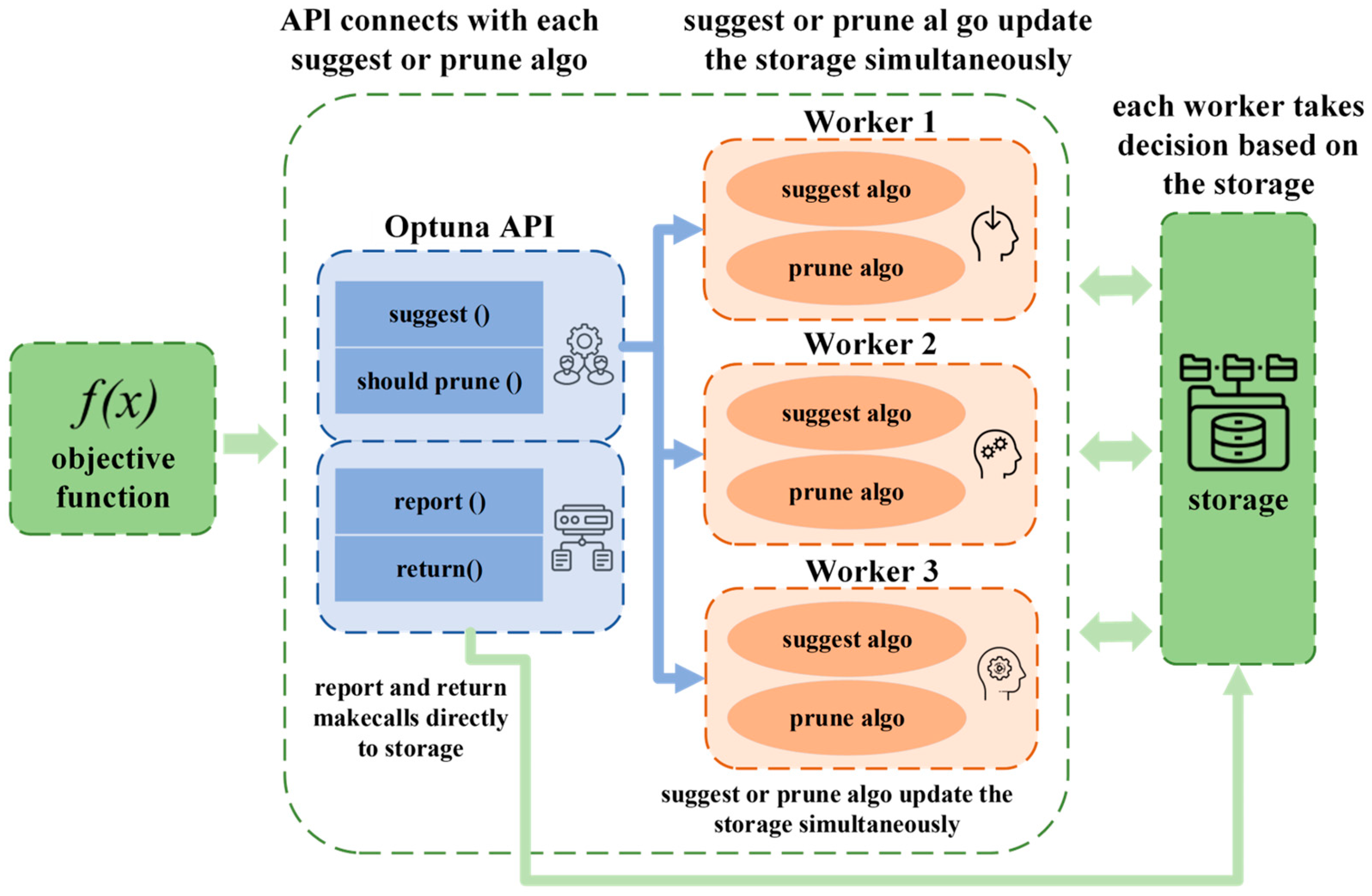
The Optuna framework (Figure 1) is an automated hyperparameter optimization tool, the core of which is to find the optimal hyperparameter configuration of a machine learning model or algorithm by using Bayesian optimization to strike a balance between efficient exploration and utilization [25,26,27].

Figure 1.
Optuna tuning framework diagram.
2.3. Construction of Optuna-Bi-LSTM-Transformer Model
2.3.1. Bi-LSTM
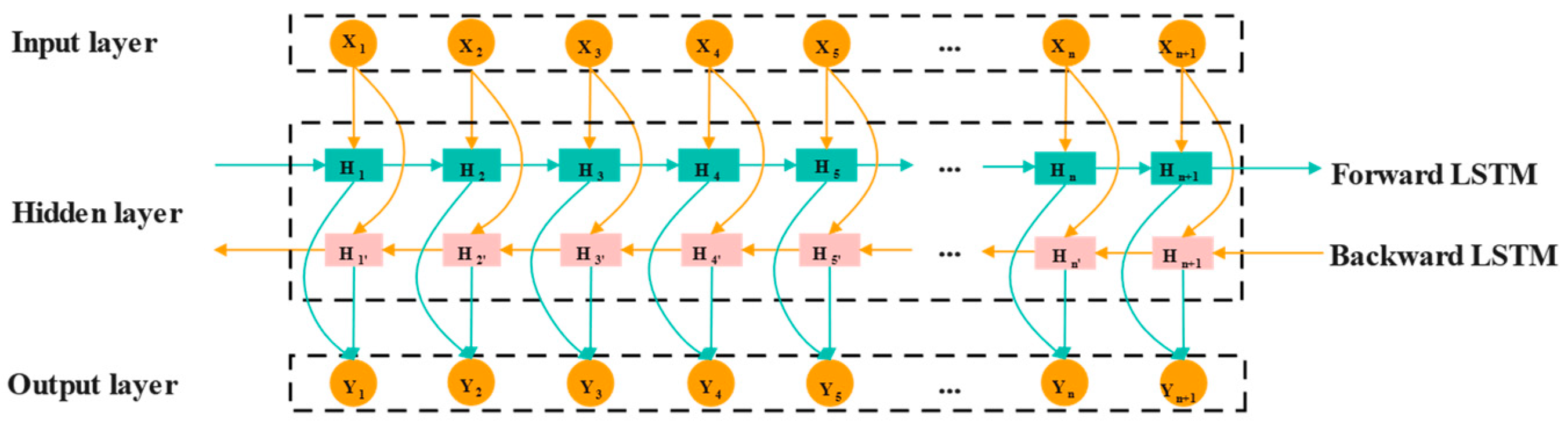
Bi-LSTM (Bidirectional Long Short-Term Memory Network) is an advanced deep learning model for time series data, combining both forward and backward LSTM networks [28,29,30]. Forward LSTM forward analysis data along sequence data; backward LSTM processes the time series in reverse to capture historical information, and this bidirectional approach allows Bi-LSTM to effectively capture long-term dependencies, improving data utilization and prediction accuracy. The network structure of Bi-LSTM is illustrated in Figure 2.
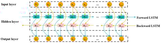
Figure 2.
Structure of Bi-LSTM neural network.
2.3.2. Transformer
Transformer is a deep learning model that relies on the attention mechanism [26]. Its architecture is shown in Figure 3. Transformer abandons the architectural limitations of recurrent neural network (RNN) or convolutional neural network (CNN) in traditional sequence models and realizes efficient sequence modeling capability through full attention mechanism [31,32,33]. The architecture of Transformer was primarily determined through a combination of theoretical insights from attention mechanisms and empirical validation, as demonstrated in the original Transformer model by Vaswani et al. [34].
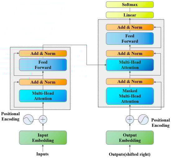
Figure 3.
Transformer architecture.
Transformers outperform RNNs for time-series prediction due to their ability to capture long-range dependencies through the self-attention mechanism, avoiding the vanishing gradient problem commonly faced by RNNs. Furthermore, the parallel processing capability of Transformers allows for more efficient computation, enabling them to model sequences as a whole rather than sequentially, which enhances their predictive power and performance.
- (1)
- Multi-head attention mechanism
Transformer’s multi-head attention mechanism (MHA) is one of its core modules, designed to capture global dependencies and multi-scale features in input features [35].
At the core of the multi-head attention mechanism is the “Self-Attention” computation, designed to create a representation of contextual features by examining the interactions among Query (Q), Key (K), and Value (V). Given an input matrix , is first generated by a linear transformation, i.e.,:
where is the learnable parameter matrix, and dk is the dimension of each attentional head. Subsequently, the dot product is used to calculate the similarity between the query and the key, resulting in an attention score:
Here, represents the similarity of the query to the key, is the scaling factor to prevent the dot product value from being too large to cause gradient instability, and is used for normalization so that the attention score at each position is a probability distribution. The attention score generates a context vector through the weighted value matrix V, which represents the global information of the input sequence.
To improve the model’s capacity to capture multi-scale features, the multi-head attention mechanism handles the input data using multiple attention heads simultaneously. Each attentional head learns the feature representation in a different subspace, and its output is as follows:
where is the parameter matrix of the I-th head. When all the attention heads have been calculated, the output is integrated by concatenation operation and the final output of multi-head attention is generated by linear transformation:
where is a parameter matrix for linear transformation after concatenation.
- (2)
- Feed Forward Network
After multiple self-attention, Transformer further enhances feature nonlinear conversion capability through feedforward neural network [34]. The features of each location are independently nonlinear and mapped through a two-layer fully connected network:
where and are trainable parameters, and is usually larger than d to increase the model capacity. , are offset terms.
- (3)
- Residual connection and layer normalization
For each sublayer, such as multi-head attention or feed-forward networks, the residual connection adds the input directly to the output:
where is the input of the sublayer and is the output of the sublayer. The residual connection allows gradients to propagate directly to the shallow network, preventing features from being weakened layer by layer in the deep network.
2.3.3. Optuna-Bi-LSTM-Transformer
The Optuna-Bi-LSTM-Transformer model is optimized using the Optuna framework to determine the optimal values of these hyperparameters, thereby maximizing the model’s performance (Algorithm 1). The process is shown in Figure 4. The specific optimization process is as follows:
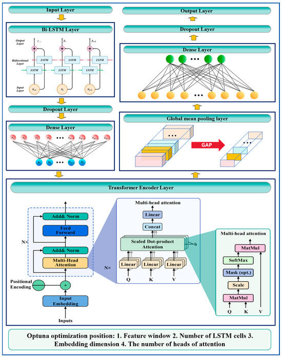
Figure 4.
Structure diagram of Optuna-Bi-LSTM-Transformer.
Step 1: Hyperparameter optimization
- Feature window size optimization: Optuna is used to search for the optimal size of the input feature window. By adjusting the length of the input sequence, OPTUNA captures the most useful information in the time series for prediction.
- LSTM unit number optimization: Optuna is employed to determine the optimal number of cells in the Bi-LSTM layer. The first Bi-LSTM layer captures local features of the input sequence, while the second layer extracts global features.
- Embedding dimension optimization: Optuna searches for the embedding dimension to balance the representation power and computational complexity of the model, ensuring that high-quality feature representations are extracted.
- Multi-head attention number optimization: Optuna is utilized to search for the optimal number of heads (num_heads) and the dimension of each head (key_dim) in the Transformer.
Step 2: Optimize the target
Goals include minimizing loss functions and improving model performance.
Step 3: Define the hyperparameter search space
By defining the search space for the aforementioned hyperparameters, Optuna is employed to efficiently optimize hyperparameters and achieve the optimal model configuration.
| Algorithm 1: Optuna-Bi-LSTM-Transformer Algorithm |
| Input: Divided and normalized feature dataset |
| Output: Best Optuna-Bi-LSTM-Transformer hyperparameters (feature_window-best, lstm_units-best, embedding_dim-best, num_heads-best) |
| 1 Start the algorithm. |
| 2 Set the Optuna objective function as: |
| 3 Optuna-Bi-LSTM-Transformer(feature_window, lstm_units, embedding_dim, num_heads). |
| 4 Initialize variables: |
| 5 lstm_units_1, lstm_units_2, num_heads, dense_units, dropout_rate, time_steps, Fitness. |
| 6 Initialize best hyperparameters: |
| 7 lstm_units_1-best, lstm_units_2-best, num_heads-best, dense_units-best, dropout_rate-best, time_steps-best, Fitness-best. |
| 8 Set loop parameters: |
| 9 max_trials, current_trial. |
| 10 Start the loop: |
| 11 from current_trial = 1 to max_trials. |
| 12 Randomly sample hyperparameters using Optuna: |
| 13 Feature_window, lstm_units, embedding_dim, num_heads. |
| 14 Compute Fitness value: 15 Fitness = Optuna-Bi-LSTM-Transformer(feature_window, lstm_units, embedding_dim, num_heads). 16 Fitness is calculated using performance metrics such as MSE, RMSE, or MAE to evaluate prediction accuracy. |
| 17 Fitness = Optuna-Bi-LSTM-Transformer(feature_window, lstm_units, embedding_dim, num_heads). |
| 18 If Fitness > Fitness-best, 19 update the following: |
| 20 Fitness-best, feature_window-best, lstm_units-best, embedding_dim-best, num_heads-best. |
| 21 Output current trial results: |
| 22 current_trial, Fitness, feature_window, lstm_units, embedding_dim, num_heads. |
| 23 If early stopping conditions are met, output: |
| 24 ‘Early stopping condition met, exiting loop’ and break the loop. |
| 25 End the loop. |
| 26 Output the best hyperparameters: |
| 27 Feature_window-best, lstm_units-best, embedding_dim-best, num_heads-best. |
| 28 End the algorithm. |
2.4. Model Analysis Method
SHAP Interpretable Model
In recent years, deep learning technology has made substantial progress, especially in handling sequential data and modeling complex relationships. Despite their strong predictive capabilities, deep learning models are often seen as “black boxes” because of their limited interpretability, which hinders their wider application.
SHapley Additive exPlanations (SHAP) is a technique for interpreting machine learning model predictions, grounded in Shapley value theory. It offers both global and local interpretability by decomposing the predicted outcomes into the contributions of each feature. It provides both global and local interpretability by breaking down the predicted outcomes into the contributions of individual features.
Based on the trained model, the SHAP interpreter is built and used to calculate the SHAP value of the test dataset. The detailed calculation formula is as follows:
3. Experiment and Analysis
3.1. Experimental Setup
3.1.1. Description of Experimental Environment and Dataset
- (a)
- Experimental Environment:
The experiments were performed using the following hardware configuration: an Intel64 Family 6 Model 154 Stepping 3 CPU with 16 GB of RAM and an NVIDIA RTX 3060 GPU with 24 GB of VRAM. The software environment consisted of the Windows 11 operating system, with TensorFlow 2.12.0 as the primary framework, and Python 3.10 as the programming language.
- (b)
- Dataset Description
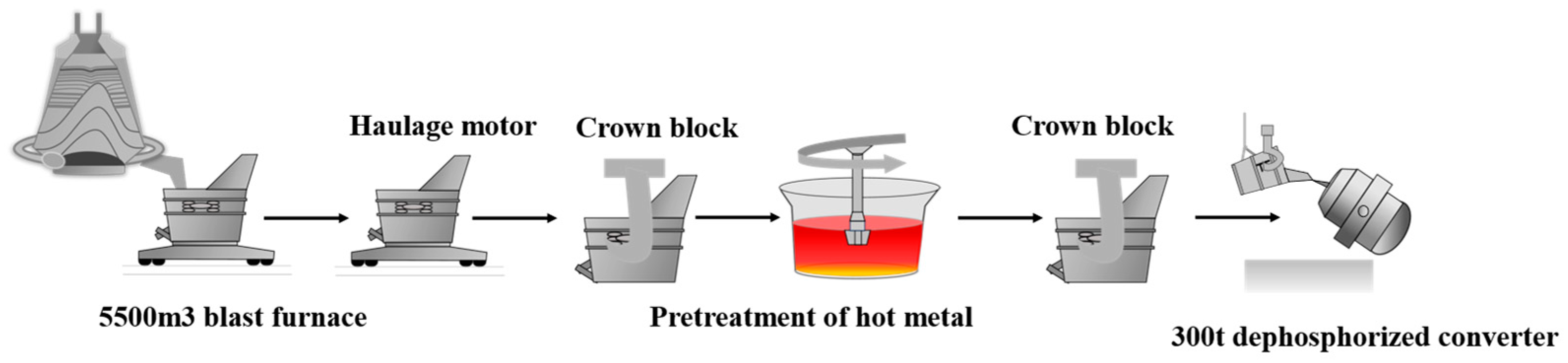
The dataset used in this study comes from Tangshan Iron and Steel Group Co., Ltd. This study utilizes hot metal ladle transportation data as its foundation, combined with the actual variation in hot metal temperature. The transportation process of molten steel ladle is shown in Figure 5. Key process parameters and time metrics of the ladle were chosen as input variables to build a predictive model for accurately forecasting the incoming station temperature of hot metal in the KR desulfurization process (KR inlet temperature). These original characteristics include the following: age (number of times), total connection duration (seconds), rewrapping time with cover (seconds), rewrapping time without cover (seconds), primary connection temperature, secondary connection temperature, secondary temperature, total net weight of hot metal ladle, empty time (with cover), empty packet interval (seconds), and KR station temperature. Considering the primary factors influencing the KR inlet temperature, six parameters were chosen as input variables: hot metal temperature at the previous station, total iron tapping duration (seconds), covered time for a loaded ladle (seconds), uncovered time for a loaded ladle (seconds), covered time for an empty ladle (seconds), and time intervals for an empty ladle (seconds). The KR inlet temperature serves as the target variable for prediction.
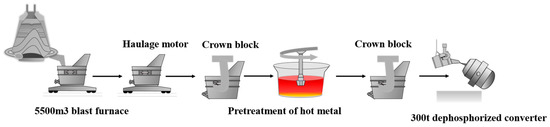
Figure 5.
Hot Metal Ladle Transportation Flowchart.
Specifically, the molten iron temperature of the previous station refers to the temperature of the previous station during the transportation of molten iron, which reflects the trend of temperature change and is crucial to the subsequent temperature prediction. Total pouring time (seconds) refers to the total time from the beginning of pouring to the completion of pouring. Full ladle covering time (s) and full ladle not covering time (s) represent the covering time and non-covering time at full ladle load, respectively. The covering time helps to reduce heat loss of molten iron and maintain a high temperature, while the non-covering time may cause the temperature to drop. Empty ladle cover time (seconds) refers to the length of time that the ladle is covered in the empty ladle state. Finally, the time interval of the empty ladle (seconds) represents the time interval of the ladle in the idle state, which is mainly related to the preparation and transfer process of the ladle, and indirectly affects the final temperature change.
3.1.2. Baseline Model
To thoroughly assess the predictive performance of the proposed Optuna-optimized Transformer-Bi-LSTM hybrid model, this study benchmarks a range of models, including Optuna-Transformer, Optuna-Transformer-Bi-LSTM, Transformer-Bi-LSTM, Optuna-Bi-LSTM, Transformer-LSTM, Transformer, LSTM, and Bi-LSTM.
3.1.3. Model Performance Evaluation Metrics
This study uses several commonly employed evaluation metrics: R2 (Coefficient of Determination), Mean Squared Error (MSE), Root Mean Squared Error (RMSE), Mean Absolute Percentage Error (MAPE), and Accuracy.
- (1)
- Coefficient of Determination (R2)
In this context, represents the actual values, represents the predicted values, denotes the mean of the actual values, and n is the total number of samples.
- (2)
- Mean Squared Error (MSE)
- (3)
- Root Mean Squared Error (RMSE)
- (4)
- Mean Absolute Percentage Error (MAPE)
- (5)
- Accuracy (Hit Rate)
Hit Rate is utilized to determine if the discrepancy between the predicted and actual values lies within a specified tolerance range, indicating the reliability and precision of the model’s predictions. In this study, assuming the error tolerance range is defined as [insert tolerance range], the Hit Rate is calculated using the following formula:
In this context, n represents the total number of samples, denotes the actual values, represents the predicted values, efers to the prediction error, and is the indicator function. When , the value of is 1, otherwise, it is 0.
3.1.4. Model Hyperparameter Configuration and Optimization
In the experiments, four key hyperparameters were chosen for optimization: feature window size, number of LSTM units, embedding dimension, and the count of heads in the multi-head attention mechanism. To evaluate the impact of hyperparameter combinations on model performance, the Mean Squared Error (MSE) of the training set was used as the objective function, with the Optuna framework facilitating the automated search and optimization process.
3.2. Data Processing and Feature Selection
3.2.1. Data Preprocessing
In light of the large-scale data characteristics in hot metal temperature prediction, the data preprocessing steps are crucial, including handling missing values, outliers, and data normalization. The turnover information of hot metal ladles from Tangshan Steel serves as the experimental base data, with nine key indicators selected as initial feature variables, among which the KR inlet temperature is set as the prediction target. These initial indicators include the following: ladle age (count), total iron tapping duration (seconds), covered time for a loaded ladle (seconds), uncovered time for a loaded ladle (seconds), primary and secondary iron tapping temperatures, hot metal temperature, total net weight of the ladle, covered time for an empty ladle, and time intervals for an empty ladle (seconds).
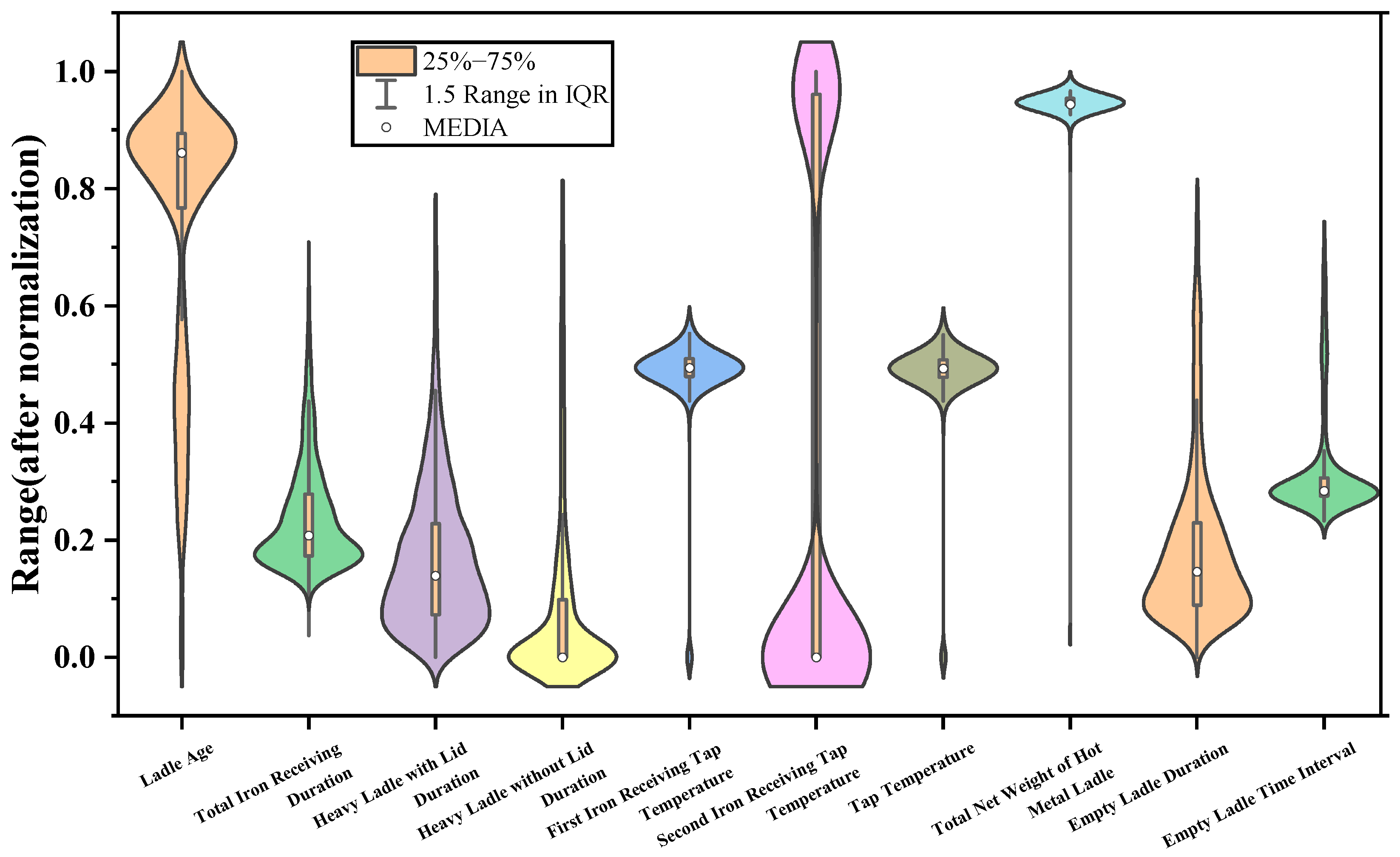
For outlier detection, a violin plot method was employed, visualizing the data distribution to identify anomalies. The violin diagram is shown in Figure 6.

Figure 6.
Violin plot.
After addressing missing values, we performed an outlier detection process. To identify potential outliers, we initially used a violin plot (Figure 6) to visually assess the distribution of the data. Any points that deviated significantly from the general distribution were flagged as outliers. These outliers were then further examined to determine whether they represented genuine data points or erroneous entries. If the outliers were deemed irrelevant or erroneous, they were removed. To ensure that the removal of outliers did not result in the loss of important information, we carefully reviewed the context of the data and cross-validated the impact of their removal on model performance. Following the outlier treatment, the Z-score normalization method was applied to standardize the data, ensuring uniformity in the dimensionality of different indicators and eliminating discrepancies in value ranges. The normalization formula used is as follows:
In this context, X represents the original data, μ is the mean, σ is the standard deviation.
3.2.2. Feature Selection
This study employed the Recursive Feature Elimination with the Cross-Validation (RFECV) method to identify six key features that significantly influence hot metal temperature prediction. These features include the following: iron tapping temperature, total iron tapping duration (seconds), covered time for a loaded ladle (seconds), uncovered time for a loaded ladle (seconds), covered time for an empty ladle, and time intervals for an empty ladle (seconds).
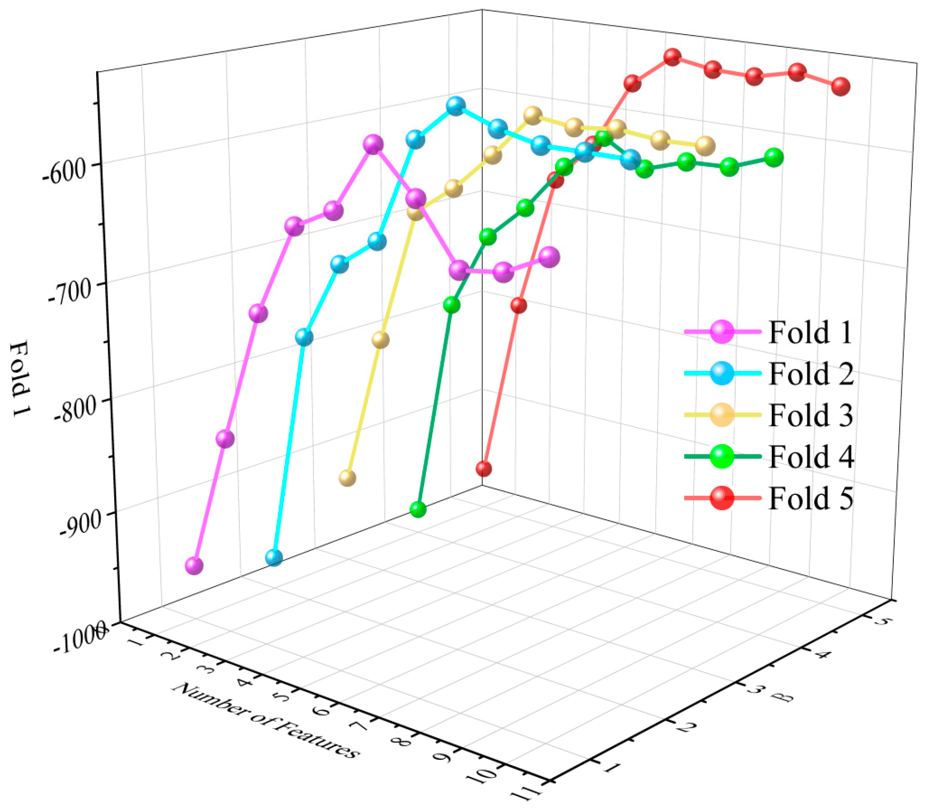
The feature selection process relies on the CatBoost regression model and employs a 5-fold cross-validation strategy. Through recursive elimination of redundant or low-correlated features, the model performance is progressively optimized. The final selection of these six features not only reduces the model’s complexity but also significantly enhances its predictive accuracy and generalization capability. As illustrated in Figure 7 and Figure 8.
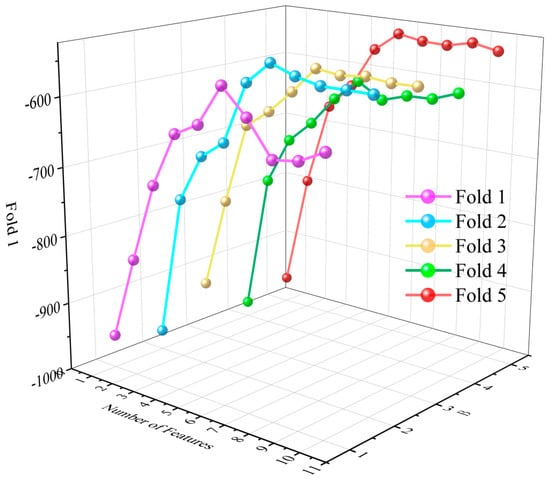
Figure 7.
Feature number and cross-validation score.
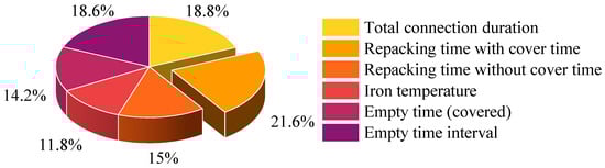
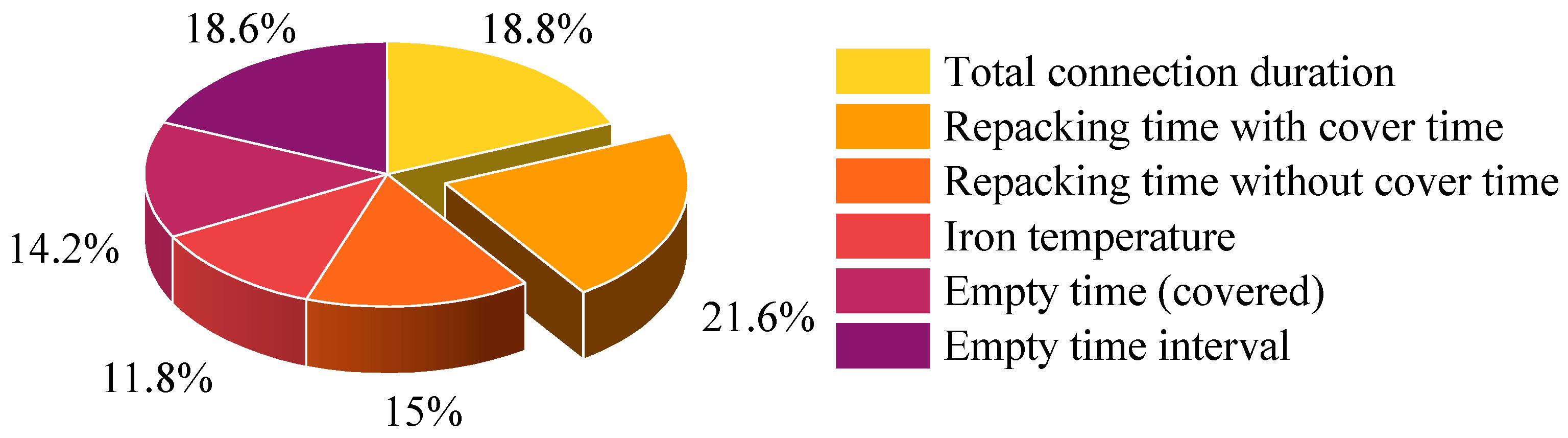
Figure 8.
Feature importance of selected features.
3.3. Experimental Results and Comparison
3.3.1. Hyperparameter Analysis of the Optuna-Transformer-Bi-LSTM Network Model
Table 1 presents the key parameter settings and their optimal choices for the Optuna-Transformer-Bi-LSTM model. These parameters, confirmed through experiments, significantly influence the model’s predictive performance. Specifically, the feature window size is set to 20. With 128 LSTM units, the Bi-LSTM layer is capable of extracting more intricate sequence features, enhancing the model’s ability to capture complex dynamic variations. The embedding dimension is set to 64, striking a good balance between feature representation power and computational efficiency. The multi-head attention mechanism is configured with eight heads.

Table 1.
Parameter settings for the Optuna-Transformer-Bi-LSTM model.
3.3.2. Ablation Study
In this study, a systematic ablation study was conducted to deeply analyze the performance and contributions of the hybrid deep learning model based on Bi-LSTM and Transformer (Table 2). Specifically, we compared the Transformer, Bi-LSTM, LSTM, and their combined models (such as Transformer-Bi-LSTM and Optuna-Transformer-Bi-LSTM). The Optuna-optimized hybrid model (Optuna-Transformer-Bi-LSTM), proposed as the core model in this study, was evaluated by comparing it with unoptimized models, single-structure models, and models optimized only with Optuna. See Appendix A for the model architecture and hyperparameters.
Table 2.
Comparison of the experimental results.
This paper monitors val_loss during training by using the early_stopping callback function. The function of the callback is to stop the training in advance if the validation loss is not improved within a certain number of rounds during the training process to prevent the model from overfitting. In the end, the paper chooses the weight of the round with the least validation loss, rather than the weight of the last round, so as to ensure the best performance of the model in generalization ability. Each model uses a different ratio of training set to test set (8:2, 7:3, 6:4), mainly to evaluate the performance and stability of the model under different data volumes.
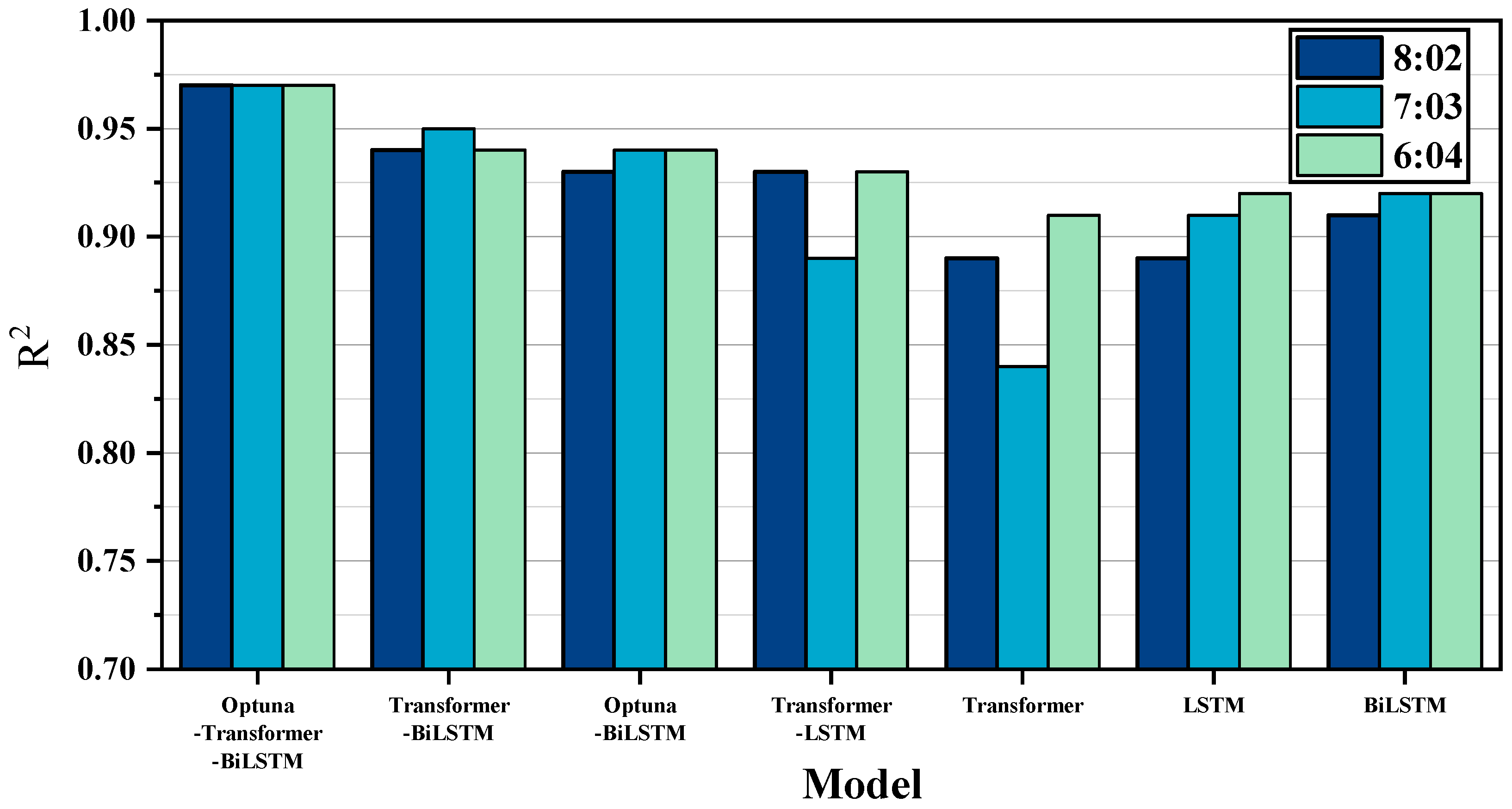
The comparison of R2 for different models, as shown in Figure 9, reveals that, across the three data divisions (8:2, 7:3, 6:4), the Optuna-Transformer-Bi-LSTM model consistently achieves the highest hit ratio within the error ranges of ±5 °C and ±10 °C. Specifically, the hit ratio for ±5 °C remains above 98%, while the ±10 °C hit rate is nearly 100%, significantly outperforming other models.
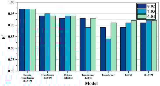
Figure 9.
Comparison of R2 for different models.
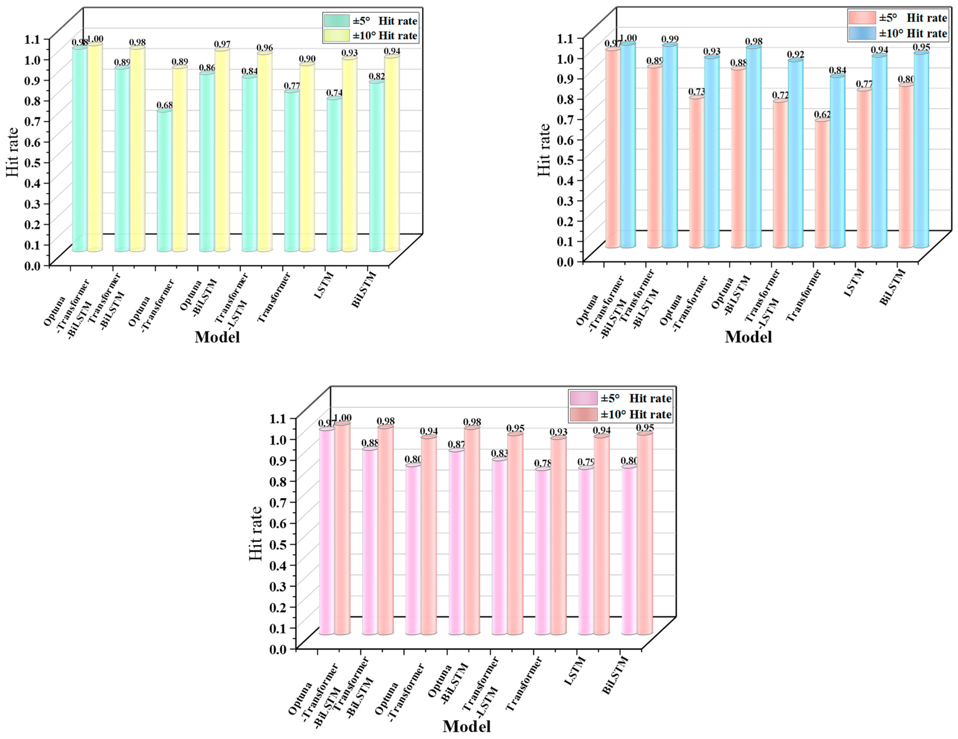
The comparison of hit rates, shown in Figure 10, demonstrates that the Optuna-Transformer-Bi-LSTM model consistently maintains the highest hit rates across the three data splits (8:2, 7:3, 6:4) within the ±5 °C and ±10 °C error ranges. The hit rate for ±5 °C exceeds 98%, and for ±10 °C, it is nearly 100%, significantly outperforming other models. In contrast, the unoptimized Transformer-Bi-LSTM model and other single-structure models, such as LSTM and Transformer, show significantly lower hit rates, especially in the ±5 °C range, where the discrepancy is more noticeable, with the lowest hit rate dropping to 74%. When calculating the hit rate, we set an error tolerance range of ±15 °C; the higher the hit rate, the better. In engineering practice, when the error between the predicted value and the actual value is within ±15 °C, the hit rate of 100% is considered to be very accurate and meets the actual production requirements.

Figure 10.
Comparison of Hit Rate under different proportions.
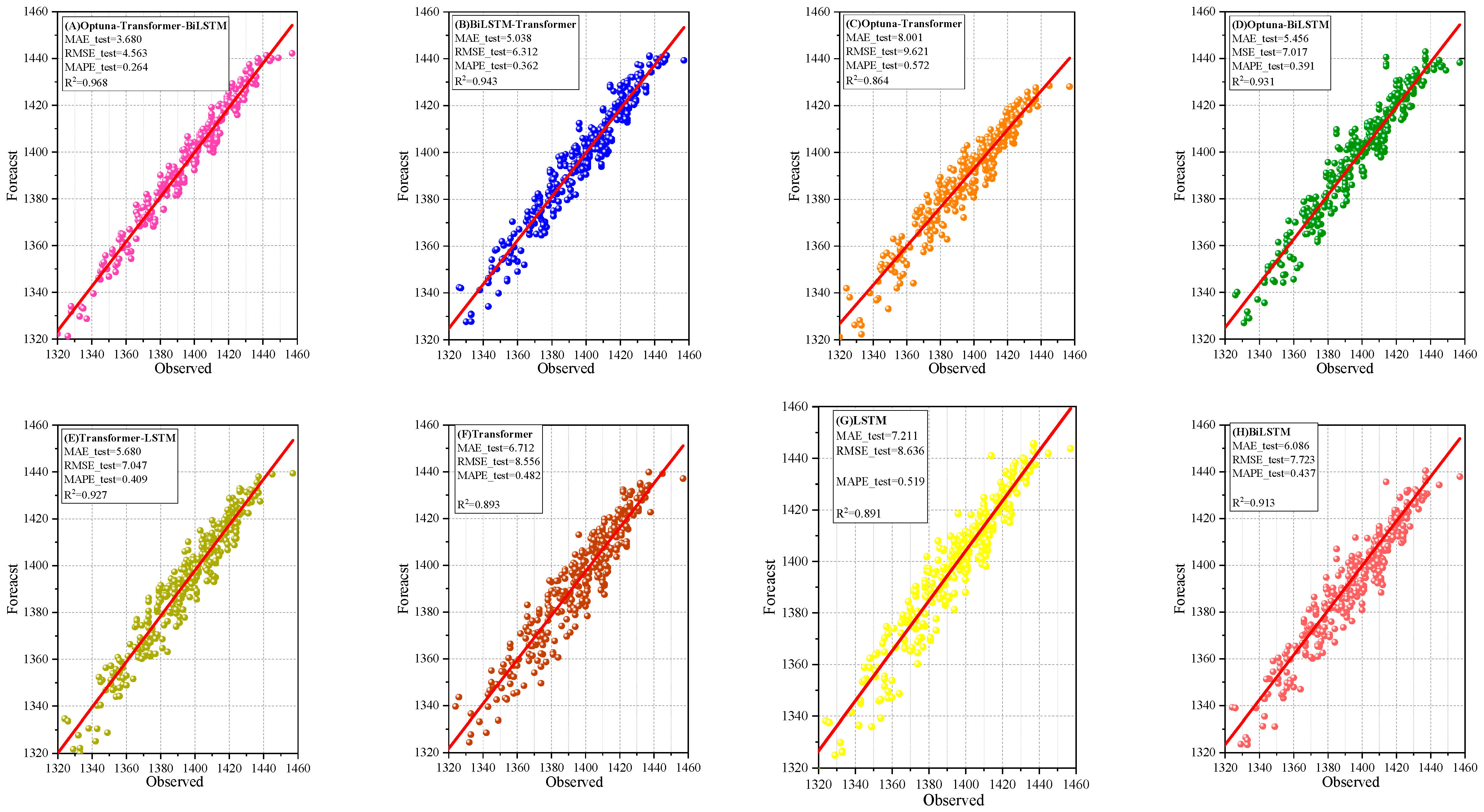
Figure 11 is an important scatter plot used to evaluate the model’s fitting ability (8:2 division of training set, test set, and dataset). The scatter plot shows that the predicted values of the Optuna-Transformer-Bi-LSTM model are very close to the actual values, with the points closely distributed around the ideal fitting line. The R2 value reaches 0.968, while both MAE and RMSE outperform those of other models, demonstrating the model’s exceptional fitting accuracy and robustness in molten iron temperature reduction prediction.
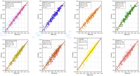
Figure 11.
Scatter plot of predicted and observed values (8:2 division of training set, test set, and dataset).
3.3.3. The Simulation Results of KR Station Entrance Temperature
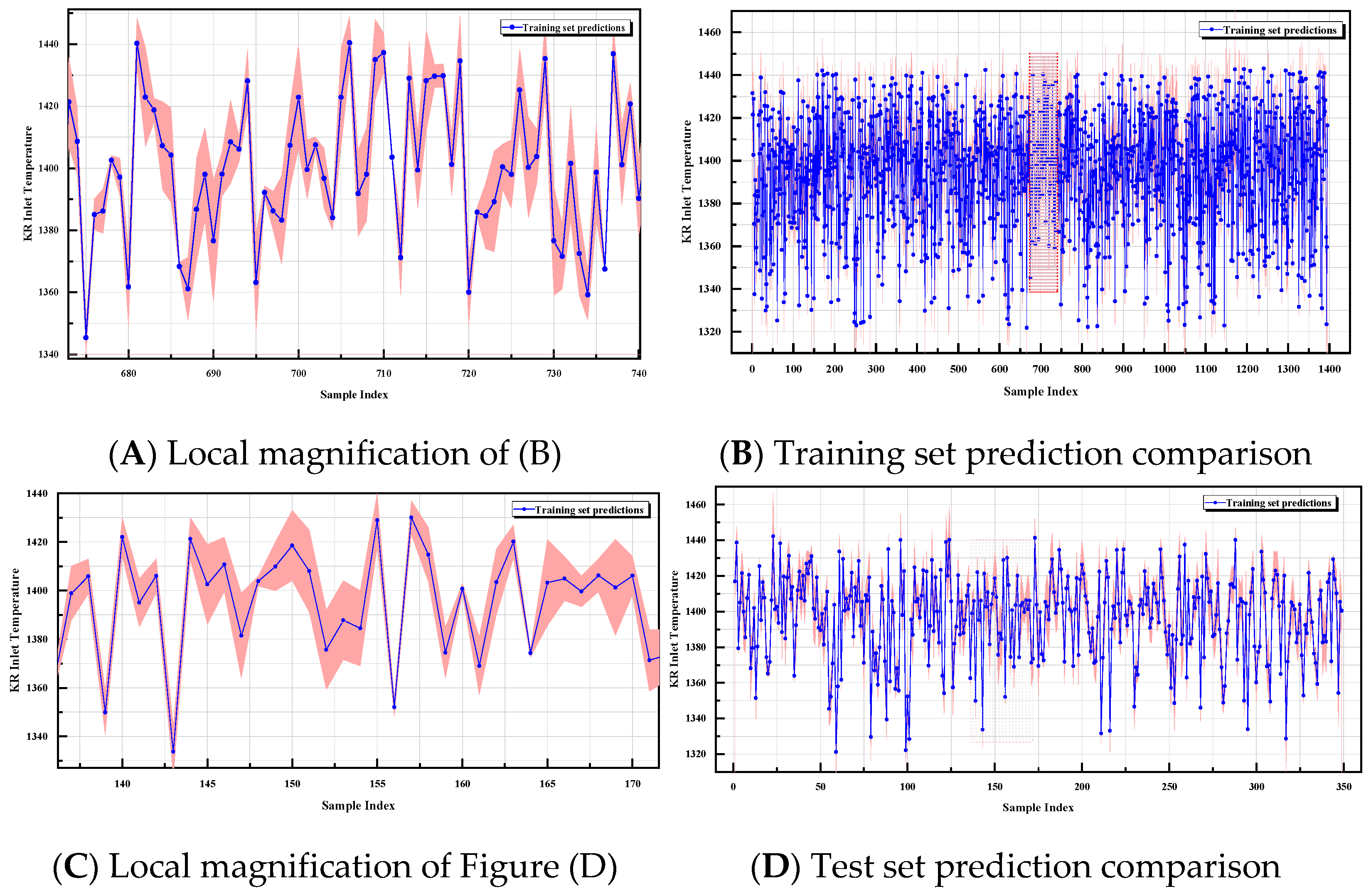
From the simulation results in Figure 12, it can be observed that the predicted values of the model exhibit a strong alignment with the actual values. The blue solid line represents the predicted values, while the pink shaded area indicates the ±10 °C prediction error range. Overall, the majority of the predicted values fall within this error range, showcasing the model’s strong predictive accuracy. Moreover, the predicted values’ fluctuations closely align with the dynamic variations in the actual values, indicating that the model effectively captures the dynamic changes in molten iron temperatures.
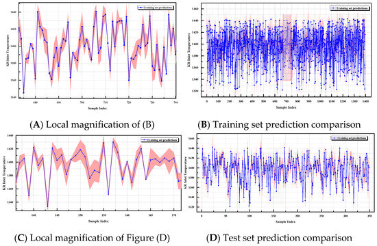
Figure 12.
Test set fit plot.
3.3.4. SHAP-Based Model Explainability Analysis
- (1)
- Global Explanation
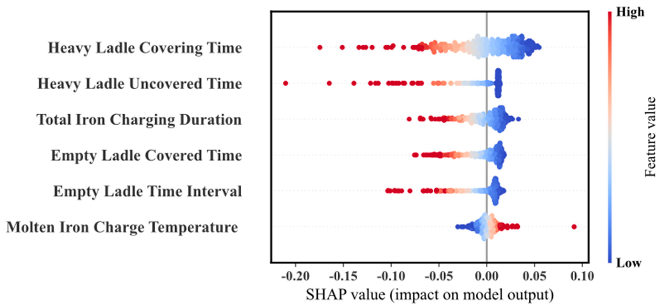
Figure 13 provides a comprehensive SHAP summary plot, illustrating the SHAP values for individual samples based on input features. After model generation, the features were ranked based on their contributions to the prediction results. The x-axis represents the SHAP values, and the y-axis lists the input features. Each point on the plot represents a sample, with the color intensity reflecting the feature value—blue denotes lower feature values, while red indicates higher feature values. The model analysis reveals that “HeavyLadleCoveringTime” and “HeavyLadleUncoveredTime” are the two most influential factors for predicting molten iron temperature, as variations in their feature values significantly affect the magnitude and sign of the SHAP values. Additionally, “TotalIron Charging Duration” also plays an important role in model performance, while “Empty Ladle Covered Time”, “EmptyLadleTimeInterval”, and “MoltenIron Charge Temperature” have relatively lower contributions. This feature importance analysis provides strong evidence for improving the accuracy of molten iron temperature prediction and optimizing related process flows.
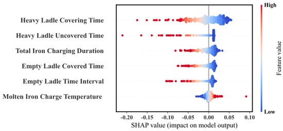
Figure 13.
SHAP summary plot.
Figure 14 illustrates the feature importance visualization of SHAP values, measuring the average influence of each input feature on the model’s prediction of molten iron ladle temperature. The x-axis represents the average absolute SHAP values, reflecting the magnitude of the feature’s impact on the model’s output, while the y-axis orders the features by their importance. Among them, “HeavyLadleCoveringTime” has the highest average SHAP value, indicating that it is the most important factor for predicting molten iron ladle temperature. Following that are “HeavyLadleUncoveredTime” and “TotalIronChargingDuration,” which also have significant effects on the model’s predictions. “EmptyLadleCoveredTime” and “EmptyLadleTimeInterval” are of moderate importance, while “MoltenIronChargeTemperature” has the least impact.
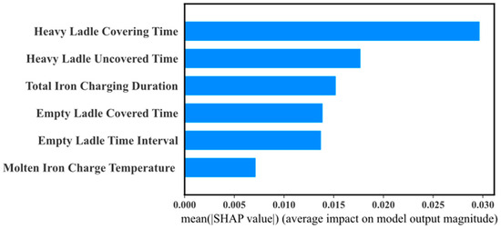
Figure 14.
SHAP value feature importance visualization.
- (2)
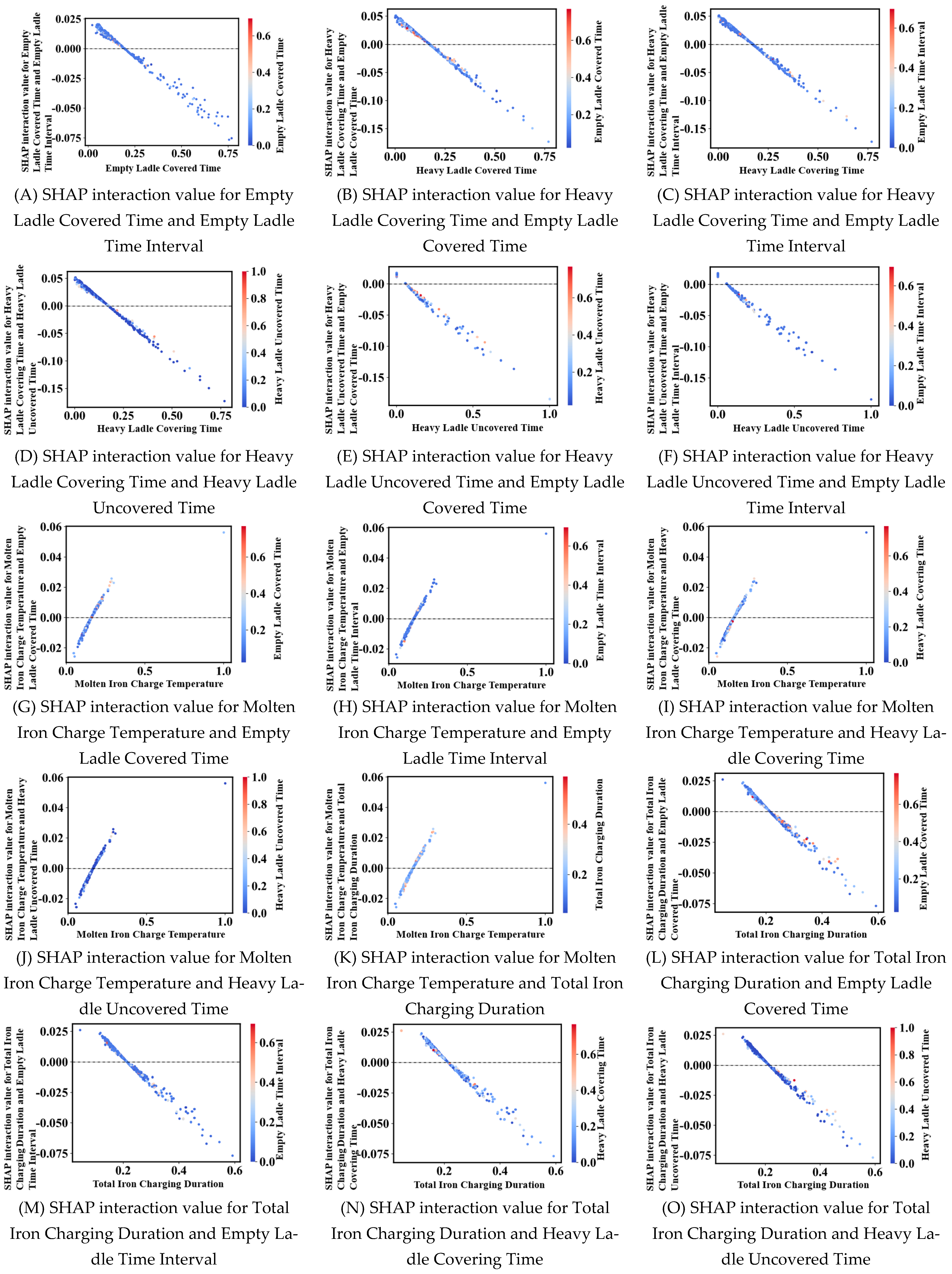
- SHAP interaction analysis
With the global interpretation, we are able to identify the overall impact of individual features on the model predictions, but further SHAP interaction analysis is required for a deeper understanding of the interactions between features and their joint contribution to the prediction results.
Interpreted as an example, Figure 15A, which shows the SHAP interaction values between the empty packet coverage time and the empty scooping sub-time interval, exhibits a negative correlation, with a gradual decrease in the SHAP interaction values as the empty packet coverage time increases and the color shifts from blue to red, which indicates an increase in the empty packet time interval.
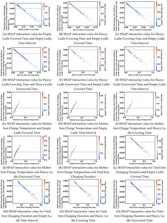
Figure 15.
SHAP interaction value plot.
- (3)
- Partial explanation
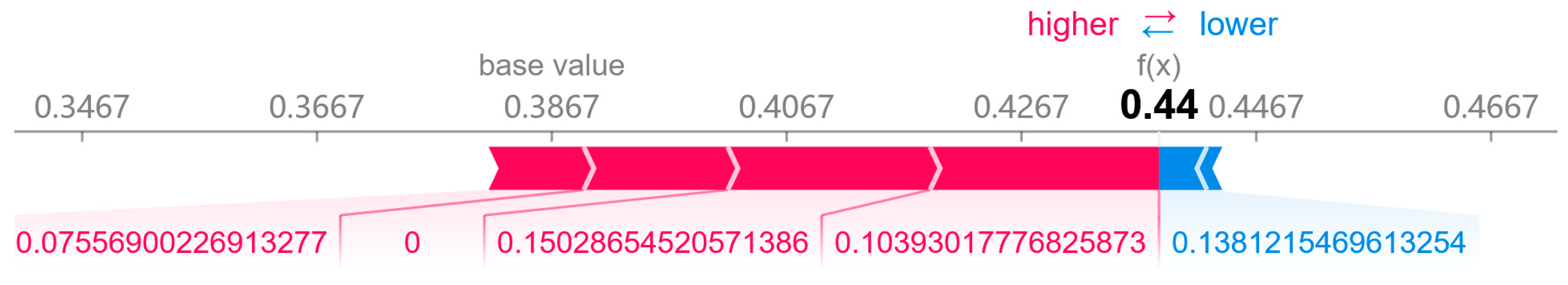
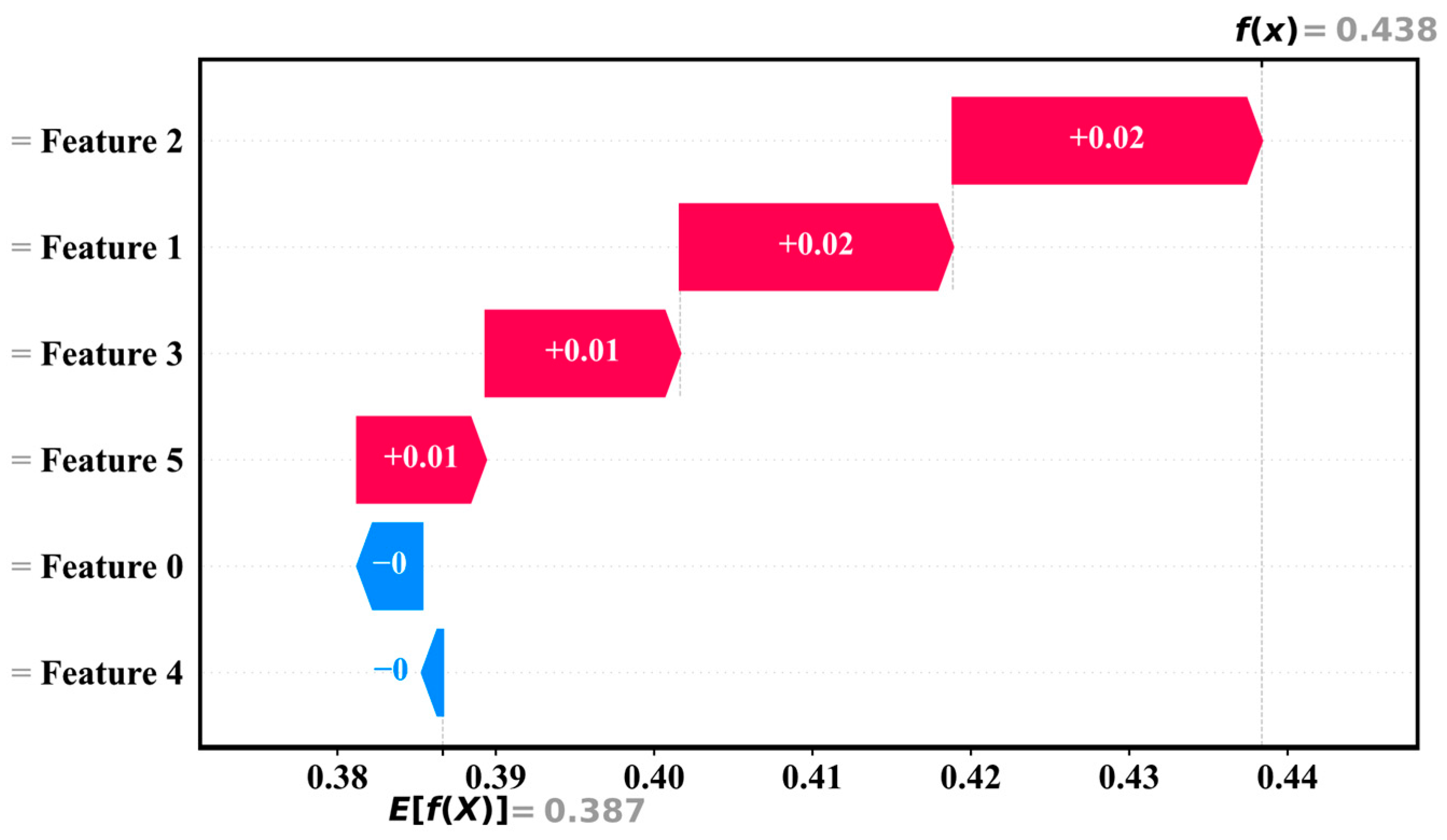
Figure 16 and Figure 17 show the force plot and waterfall plot, respectively, which are used to locally interpret the origin of individual sample predictions and the specific contribution of each feature to the prediction.
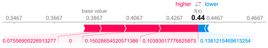
Figure 16.
Force diagram.

Figure 17.
Waterfall diagram.
In Figure 16, the force diagram shows the effect of each feature on the predicted value f(x) = 0.44 by visualizing the positive (red arrows) and negative (blue arrows) contributions of the features. The baseline value (base value) is 0.3867, representing the initial predicted value of the model without any feature inputs. Red arrows (positive contribution) indicate that the value of the feature shifts the prediction upwards, while blue arrows (negative contribution) represent that it pulls the prediction downwards. For example, the total contribution of a particular combination of features to the final output of the model is +0.0533, which raises the final prediction to 0.44.
In Figure 17, the waterfall plot further quantifies and demonstrates step-by-step the process of forming the predicted values. Each feature is represented as a stacked representation of its incremental impact on the predicted value. The baseline value is also 0.387, and by stacking the contributions of each feature in turn (e.g., Feature 2 and Feature 1 each contribute +0.02+0.02, and Feature 3 and Feature 5 each contribute +0.01+0.01), the final predicted value is obtained as f(x) = 0.438 f(x) = 0.438.
3.3.5. Analysis and Discussion
In this study, the proposed hybrid deep learning model based on Bi-LSTM and Transformer shows obvious advantages in the prediction of hot metal temperature. Compared to existing traditional methods, our approach has achieved significant improvements in accuracy, efficiency, and interpretability. First of all, the combination of Bi-LSTM and Transformer enables the model to effectively capture local features and global dependencies in time series data. Bi-LSTM can make full use of historical information and future trends through its bidirectional structure, while Transformer can handle long-distance dependencies through its global attention mechanism. Thus, the overall prediction accuracy of the model is improved. This combination makes our model better able to deal with complex nonlinear data, and shows high accuracy in the prediction of hot metal temperature.
4. Conclusions
This paper addresses the challenge of molten iron temperature drop prediction during the transit process and the limitations of traditional methods in handling high-dimensional data and ensuring model generalization. We propose an interpretable hybrid deep learning model that combines Bi-LSTM and Transformer to effectively capture both local and long-range dependencies. The model’s interpretability is ensured through SHAP analysis, which quantifies the contribution of each input feature to the prediction outcomes, enhancing transparency. The experimental results demonstrate that our proposed model outperforms traditional models in R2, RMSE, MAE, and hit rate metrics, confirming its effectiveness in predicting molten iron temperature drops. Furthermore, the SHAP analysis reveals the key factors influencing the temperature drop of the iron ladle, providing actionable insights for optimizing iron transfer scheduling. Future work will focus on incorporating additional real-time operational data and environmental factors to improve the model’s robustness. Additionally, we plan to explore adaptive learning techniques to enhance model performance under varying production conditions, aiming for seamless deployment in industrial applications. Furthermore, expanding the model’s interpretability framework will help stakeholders better understand its decision-making process, promoting its integration into real-world temperature management systems.
Author Contributions
Conceptualization, Z.S.; methodology, Z.S. and W.H.; software, Z.S.; validation, Z.S.; formal analysis, Z.S.; data curation, Z.S., Y.Z. and J.H.; writing—original draft, Z.S.; writing—review and editing, W.H. and Y.H.; supervision, W.H. and Y.H.; project administration, W.H. All authors have read and agreed to the published version of the manuscript.
Funding
This research received no external funding.
Data Availability Statement
The datasets presented in this article are not readily available because the data are part of an ongoing study. Requests to access the datasets should be directed to the corresponding author.
Acknowledgments
This research was conducted independently without external funding support. The author is grateful to all individuals who provided valuable insights and assistance during the research process.
Conflicts of Interest
The authors declare that they have no known competing financial interests or personal relationships that could have influenced the work reported in this study.
Appendix A. Model Architecture and Hyperparameters
| Model | Parameter | Numeric Value |
| Optuna-Transformer-Bi-LSTM | Embedding Dimension | 64 |
| Feature Window Size | 20 | |
| Number of LSTM Units | 128 | |
| Dropout | 0.2 | |
| Num_heads | 8 | |
| key_dim | 64 | |
| Learning rate | CosineDecay scheduling | |
| Weight_decay | 0.0002 | |
| Patience | 10 | |
| Factor | 0.5 | |
| Batch size | 25 | |
| Epochs | 50 | |
| Validation_split | 0.2 | |
| Transformer-Bi-LSTM | Embedding Dimension | 32 |
| Number of LSTM Units | 128 | |
| Dropout | 0.1 | |
| Num_heads | 4 | |
| key_dim | 64 | |
| Learning rate | CosineDecay scheduling | |
| Weight_decay | 0.0001 | |
| Patience | 10 | |
| Factor | 0.5 | |
| Batch size | 25 | |
| Epochs | 50 | |
| Validation_split | 0.2 | |
| Feature Window Size | 25 | |
| Transformer-LSTM | Number of LSTM Units | 64 |
| Learning rate | 0.01 | |
| Batch size | 32 | |
| Epochs | 14 | |
| Number of Transformer blocks | 2 | |
| Num_heads | 4 | |
| Key_dim | 32 | |
| Dropout | 0.1 | |
| Time_steps | 10 | |
| Embedding_activation | relu | |
| Optuna-Transformer | Activation | Adam |
| Dropout | 0.1 | |
| Batch size | 35 | |
| Num_blocks | 3 | |
| Epochs | 40 | |
| Validation_split | 0.3 | |
| Num_heads | 8 | |
| Dense_dim | 64 | |
| Embed_dim | 32 | |
| Transformer | Activation | Adam |
| Dropout | 0.1 | |
| Batch size | 32 | |
| Num_blocks | 3 | |
| Epochs | 36 | |
| Validation_split | 0.2 | |
| Num_heads | 4 | |
| Dense_dim | 64 | |
| Embed_dim | 32 | |
| Optuna-Bi-LSTM | Activation | Adam |
| Dropout | 0.1 | |
| The number of neurons in the LSTM layer | 64 | |
| Learning rate | 0.001 | |
| Batch size | 25 | |
| Epochs | 7 | |
| Bi-LSTM | Activation | Adam |
| Dropout | 0.1 | |
| The number of neurons in the LSTM layer | 64 | |
| Learning rate | 0.001 | |
| Batch size | 20 | |
| Epochs | 9 | |
| LSTM | Activation | Tanh |
| LSTM Number of layers | 2 | |
| Dropout | 0.2 | |
| Learning rate | 0.001 | |
| Batch size | 32 | |
| Epochs | 100 |
References
- Li, X.; Sun, W.; Zhao, L.; Cai, J. Material metabolism and environmental emissions of BF-BOF and EAF steel production routes. Miner. Process. Extract. Metall. Rev. 2018, 39, 50–58. [Google Scholar] [CrossRef]
- Wang, Z.L.; Bao, Y.P. New steelmaking process based on clean deoxidation technology. Int. J. Miner. Metall. Mater. 2024, 31, 1249–1262. [Google Scholar] [CrossRef]
- Durdán, M.; Terpák, J.; Laciak, M.; Kacur, J.; Flegner, P.; Tréfa, G. Hot metal temperature prediction during desulfurization in the ladle. Metals 2024, 14, 1394. [Google Scholar] [CrossRef]
- Zhao, J.; Li, X.; Liu, S.; Wang, K.; Lyu, Q.; Liu, E. Prediction of hot metal temperature based on data mining. High Temp. Mater. Process. 2021, 40, 87–98. [Google Scholar]
- He, F.; He, D.-f.; Xu, A.-j.; Wang, H.-b.; Tian, N.-Y. Hybrid model of molten steel temperature prediction based on ladle heat status and artificial neural network. J. Iron Steel Res. Int. 2014, 21, 181–190. [Google Scholar] [CrossRef]
- Song, X.; Meng, Y.; Liu, C.; Yang, Y.; Song, D. Prediction of Molten Iron Temperature in the Transportation Process of Torpedo Car. ISIJ Int. 2021, 61, 1899–1907. [Google Scholar] [CrossRef]
- Zhang, X.; Kano, M.; Matsuzaki, S. Ensemble pattern trees for predicting hot metal temperature in blast furnace. Comput. Chem. Eng. 2019, 121, 442–449. [Google Scholar] [CrossRef]
- Su, X.; Zhang, S.; Yin, Y.; Xiao, W. Prediction model of hot metal temperature for blast furnace based on improved multi-layer extreme learning machine. Int. J. Mach. Learn. Cybern. 2019, 10, 2739–2752. [Google Scholar] [CrossRef]
- Liu, D.; Tang, J.; Chu, M.; Xue, Z.; Shi, Q.; Feng, J. Hot Metal Temperature Prediction Technique Based on Feature Fusion and GSO-DF. ISIJ Int. 2024, 64, 1881–1892. [Google Scholar] [CrossRef]
- Díaz, J.; Fernández, F.J.; Prieto, M.M. Hot Metal Temperature Forecasting at Steel Plant Using Multivariate Adaptive Regression Splines. Metals 2019, 10, 41. [Google Scholar] [CrossRef]
- Yang, G.; Xu, H. A Residual Bi-LSTM Model for Named Entity Recognition. IEEE Access 2020, 8, 227710–227718. [Google Scholar] [CrossRef]
- Zhang, Y.; Yang, J. Chinese NER using lattice LSTM. arXiv 2018, arXiv:1805.02023. [Google Scholar]
- Chiu, J.P.C.; Nichols, E. Named entity recognition with bidirectional LSTM-CNNs. Trans. Assoc. Comput. Linguist. 2016, 4, 357–370. [Google Scholar] [CrossRef]
- Pinasthika, K.; Laksono, B.S.P.; Irsal, R.B.P.; Shabiyya, S.H.; Yudistira, N. SparseSwin: Swin transformer with sparse transformer block. Neurocomputing 2024, 580, 127433. [Google Scholar] [CrossRef]
- Yao, D.; Shao, Y. A data efficient transformer based on Swin Transformer. Vis. Comput. 2023, 40, 2589–2598. [Google Scholar] [CrossRef]
- Shih, Y.-J.; Wu, S.-L.; Zalkow, F.; Müller, M.; Yang, Y.H. Theme transformer: Symbolic music generation with theme-conditioned transformer. IEEE Trans. Multimed. 2022, 25, 3495–3508. [Google Scholar] [CrossRef]
- Akiba, T.; Sano, S.; Yanase, T.; Ohta, T.; Koyama, M. Optuna: A next-generation hyperparameter optimization framework. In Proceedings of the 25th ACM Sigkdd International Conference on Knowledge Discovery & Data Mining, Anchorage, AK, USA, 4–8 August 2019; pp. 2623–2631. [Google Scholar]
- Shekhar, S.; Bansode, A.; Salim, A. A Comparative study of Hyper-Parameter Optimization Tools. In Proceedings of the 2021 IEEE Asia-Pacific Conference on Computer Science and Data Engineering (CSDE), Brisbane, QLD, Australia, 8–10 December 2021; pp. 1–6. [Google Scholar]
- Koushik, A.; Manoj, M.; Nezamuddin, N. Explaining deep learning-based activity schedule models using SHapley Additive exPlanations. Transp. Lett. 2024, 1–16. [Google Scholar] [CrossRef]
- Su, R.; Liu, X.; Wei, L. MinE-RFE: Determine the optimal subset from RFE by minimizing the subset-accuracy–defined energy. Brief. Bioinform. 2020, 21, 687–698. [Google Scholar] [CrossRef]
- Zhou, X.; Wen, H.; Zhang, Y.; Xu, J.; Zhang, W. Landslide susceptibility mapping using hybrid random forest with GeoDetector and RFE for factor optimization. Geosci. Front. 2021, 12, 101211. [Google Scholar] [CrossRef]
- Benjamin, K.J.M.; Katipalli, T.; Paquola, A.C.M.; Robinson, P. dRFEtools: Dynamic recursive feature elimination for omics. Bioinformatics 2023, 39, btad513. [Google Scholar] [CrossRef]
- Yue, G. Screening of lung cancer serum biomarkers based on Boruta-shap and RFC-RFECV algorithms. J. Proteom. 2024, 301, 105180. [Google Scholar] [CrossRef]
- Shi, K.; Shi, R.; Fu, T.; Lu, Z.; Zhang, J. A Novel Identification Approach Using RFECV–Optuna–XGBoost for Assessing Surrounding Rock Grade of Tunnel Boring Machine Based on Tunneling Parameters. Appl. Sci. 2024, 14, 2347. [Google Scholar] [CrossRef]
- Fu, B.; Liang, Y.; Lao, Z.; Sun, X.; Li, S.; He, H.; Sun, W.; Fan, D. Quantifying scattering characteristics of mangrove species from Optuna-based optimal machine learning classification using multi-scale feature selection and SAR image time series. Int. J. Appl. Earth Obs. Geoinf. 2023, 122, 103446. [Google Scholar] [CrossRef]
- Li, Y.; Cao, Y.; Yang, J.; Wu, M.; Yang, A.; Li, J. Optuna-DFNN: An Optuna framework driven deep fuzzy neural network for predicting sintering performance in big data. Alex. Eng. J. 2024, 97, 100–113. [Google Scholar] [CrossRef]
- Wakjira, T.G.; Alam, M.S. Peak and ultimate stress-strain model of confined ultra-high-performance concrete (UHPC) using hybrid machine learning model with conditional tabular generative adversarial network. Appl. Soft Comput. 2024, 154, 111353. [Google Scholar] [CrossRef]
- Yang, L.; Lei, J.; Cheng, M.; Ding, Z.; Li, S.; Zeng, Z. Memristor-based circuit design of Bi-LSTM network. Neural Netw. 2025, 181, 106780. [Google Scholar] [CrossRef]
- Kulshrestha, A.; Krishnaswamy, V.; Sharma, M. Bayesian Bi-LSTM approach for tourism demand forecasting. Ann. Tour. Res. 2020, 83, 102925. [Google Scholar] [CrossRef]
- Wei, J.; Liao, J.; Yang, Z.; Wang, S.; Zhao, Q. Bi-LSTM with Multi-Polarity Orthogonal Attention for Implicit Sentiment Analysis. Neurocomputing 2020, 383, 165–173. [Google Scholar] [CrossRef]
- Ekvall, M.; Truong, P.; Gabriel, W.; Wilhelm, M.; Käll, L. Prosit Transformer: A transformer for Prediction of MS2 Spectrum Intensities. J. Proteome Res. 2022, 21, 1359–1364. [Google Scholar] [CrossRef] [PubMed]
- Gao, L.; Zhang, J.; Yang, C.; Zhou, Y. Cas-VSwin transformer: A variant swin transformer for surface-defect detection. Comput. Ind. 2022, 140, 103689. [Google Scholar] [CrossRef]
- Li, Y.; Ge, L.; Jiang, M. Fine-grained personalized federated learning via transformer in the transformer framework. Knowl-Based Syst. 2024, 301, 112276. [Google Scholar] [CrossRef]
- Vaswani, A.; Shazeer, N.; Parmar, N.; Uszkoreit, J.; Jones, L.; Gomez, A.N.; Kaiser, L.; Polosukhin, I. Attention Is All You Need. arXiv 2017, arXiv:1706.03762. [Google Scholar]
- Khan, A.; Lee, B. DeepGene Transformer: Transformer for the gene expression-based classification of cancer subtypes. Expert Syst. Appl. 2023, 226, 120047. [Google Scholar] [CrossRef]


Disclaimer/Publisher’s Note: The statements, opinions and data contained in all publications are solely those of the individual author(s) and contributor(s) and not of MDPI and/or the editor(s). MDPI and/or the editor(s) disclaim responsibility for any injury to people or property resulting from any ideas, methods, instructions or products referred to in the content. |
© 2025 by the authors. Licensee MDPI, Basel, Switzerland. This article is an open access article distributed under the terms and conditions of the Creative Commons Attribution (CC BY) license (https://creativecommons.org/licenses/by/4.0/).