Mathematical Modeling and Parameter Estimation of Lane-Changing Vehicle Behavior Decisions

Abstract

Lane changing is a crucial scenario in traffic environments, and accurately recognizing and predicting lane-changing behavior is essential for ensuring the safety of both autonomous vehicles and drivers. Through considering the multi-vehicle information interaction characteristics in lane-changing behavior for vehicles and the impact of driver experience needs on lane-changing decisions, this paper proposes a lane-changing model for vehicles to achieve safe and comfortable driving. Firstly, a lane-changing intention recognition model incorporating interaction effects was established to obtain the initial lane-changing intention probability of the vehicles. Secondly, by accounting for individual driving styles, a lane-changing behavior decision model was constructed based on a Gaussian mixture hidden Markov model (GMM-HMM) along with a parameter estimation method. The initial lane-changing intention probability serves as the input for the decision model, and the final lane-changing decision is made by comparing the probabilities of lane-changing and non-lane-changing scenarios. Finally, the model was validated using real-world data from the Next Generation Simulation (NGSIM) dataset, with empirical results demonstrating its high accuracy in recognizing and predicting lane-changing behavior. This study provides a robust framework for enhancing lane-changing decision making in complex traffic environments.

1. Introduction

Lane-changing behavior is a complex process of multi-information fusion and decision making. It tends to last only 3 s, resulting in high risk because of it increasing the workload and pressure on drivers [1]. Data indicate that traffic accidents caused by lane-changing behavior take up about $5\%$ of the traffic accident rate and $7\%$ of accidental deaths [2,3,4]. However, if drivers are warned 0.5 s before the accident, the accident rate could be reduced by $60\%$. If the warning time is advanced to 1 s, it could be reduced by 90% [5,6,7]. Therefore, it is necessary to acquire lane-changing information in enough time to improve driving safety. An assistant driving system could help play this role. From 2022, lane-keeping assistant systems and other safety technologies will become mandatory for new European vehicles; thus, assistant driving will become a vital part of the driving process [8,9].

The recognition and prediction of lane-changing behavior is a crucial application of assistant driving. With the development of vehicle technology, advanced sensing devices—such as Vehicle-to-Vehicle (V2V), Vehicle-to-Roadside (V2R), and Vehicle-to-Infrastructure (V2I)—make information sharing and passing possible between vehicles (as well as between vehicles and the surrounding environment). All of these devices support the real-time transmission of information. According to the US Department of Transportation research, V2V systems can avoid 81% of light vehicle accidents and 71% of heavy vehicle accidents, while V2I systems can avoid 26% of traffic accidents [10]. Therefore, the effective identification and prediction of vehicle lane-changing behavior is becoming an urgent task in technology research [11,12].

The core of lane-changing behavior recognition and prediction is in establishing a lane-changing behavior model [13,14,15,16,17]. The Gipps model was the first model to describe the lane-changing process of vehicles. This model took deceleration as a decisive indicator and proposed lane-changing intention, lane-changing conditions, and three safety distances parameters [18]. Following this, Schakel et al. [19] integrated this lane-changing model and car-following model to form a micro driver model. UIbrich et al. [20] established lane-changing behavior decisions based on a partially observable Markov process in a discrete space. Li et al. [21] proposed an algorithm combining HMM and Bayesian filtering to recognize a driver’s lane-changing intentions, where the HMM output serves as an initial classification of driving behavior, which then becomes the input sequence for BF, enabling the final classification of the HMM output behavior. Shuo et al. [22] developed a vehicle lane-changing prediction model based on game theory and deep learning. Xia et al. [23] proposed a human-like lane-changing intention understanding model for autonomous driving, simulating the selective attention mechanism of the human visual system and the driver’s focus on surrounding vehicles to identify lane-changing intentions. To address the issues of low recognition rates and poor real-time performance, Yu et al. [24] proposed a traffic safety solution based on deep learning for a mixed use of autonomous and manual vehicles in 5G intelligent transportation systems, thus improving lane-changing problems in mixed traffic environments. Khelfa et al. [25] used trajectory data from European two-lane highways to empirically compare different machine and ensemble learning classification techniques with a rule-based model. This analysis relied on the instantaneous measurements of up to 24 spatiotemporal variables for 4 adjacent vehicles on current and adjacent lanes. David et al. [26] reviewed and conducted a comparative analysis of machine learning methods for predicting and identifying lane-changing behavior. Li et al. [27] designed a hierarchical model to achieve accurate and early inference of driving intentions. They proposed a new module based on a parallel recursive neural network to generate intention probabilities and introduced a Gaussian hidden Markov model to replace traditional ratio comparison for determining intention output.

Vehicle lane-changing behavior decision making requires high real-time performance and accuracy [13,21,28,29]. The hidden Markov model is simple to compute, has high precision, and requires less training data, making it uniquely advantageous in handling time series. However, vehicle movement is a continuous-time behavior, and its motion observation state is not simply a limited division. Using discrete representation significantly reduces the characteristics of the original data, lowering the final accuracy. Therefore, a method capable of continuous data representation is needed to maximize the preservation of original data features and to improve model recognition accuracy. The Gaussian mixture model (GMM), which is obtained by linearly superimposing multiple single Gaussian distribution models, can approximate any continuous distribution feature and has good mathematical properties and computational performance. Therefore, combining it with HMM to form a Gaussian mixture hidden Markov model [30] was used to recognize vehicle lane-changing behavior and to, ultimately, decide whether to change lanes. Omveer et al. [31] developed and evaluated a novel hierarchical software architecture for predicting lane-changing behavior on highways. This model employs a two-layer hierarchical structure, with the first layer based on support vector machine and the second layer based on a continuous hidden Markov model combined with a Gaussian mixture model.

In this study, we focused on vehicle lane-changing behavior decision making and have made several key contributions. First, we constructed a lane-changing intention recognition model that considers the interaction effects between variables to determine the initial probability of lane changing. Second, recognizing that drivers of the vehicles may retake control based on personal preferences, we introduced driving style as a critical factor into the lane-changing decision model, resulting in a lane-changing behavior decision model based on driving styles. This model enhances decision making by aligning with individual driving habits and preferences. Finally, we validated the proposed model using real-world vehicle data from the US-101 and I-80 sections of the NGSIM dataset, demonstrating its accuracy and effectiveness through numerical analysis. By integrating driving styles into the decision-making process and validating the model with empirical data, this study advances the understanding of lane-changing behavior and provides a practical framework for improving decision making in vehicles.

The remainder of this paper is organized as follows. Section 2 introduces the proposed methods, including the construction of the lane-changing intention recognition model, the incorporation of driving styles, the construction and parameter estimation of the lane-changing behavior decision model, and the calculation of the final decision. In Section 3, the results of the empirical analysis, the values of the parameter estimation, and the final decision result are given. Finally, this study is concluded in Section 4.

2. Methodology

2.1. Recognition of the Lane-Changing Intent for Connected and Automated Vehicles

Vehicles undergo a lane-changing intention recognition process before making a final lane-changing decision, where they assess the surrounding traffic environment to determine whether a lane change is feasible. Given that connected and automated vehicles can utilize advanced wireless communication technology to achieve comprehensive V2X dynamic real-time information exchange and sharing, this study firstly aimed to extract the influencing factors of the lane-changing process for intelligent and connected vehicles, as well as aimed to establish a model for recognizing lane-changing intentions.

2.1.1. Model Variables for Lane-Changing Behavior

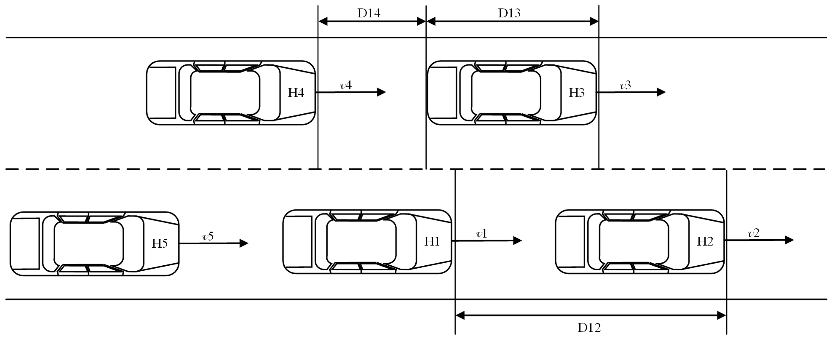
During the lane-changing process, the selection of research variables is complex due to numerous influencing factors. With the development of connected and automated vehicle technology, it has become easier to obtain vehicle trajectory information. Utilizing this real-time data allows for the study of lane-changing behavior with vehicles [32]. By analyzing both the original and target lanes, we can consider changes in the relative position of vehicles during longitudinal movement. Additionally, lane-changing behavior is influenced by vehicle speed. If the vehicle in the target lane is traveling too fast, considering only the longitudinal distance poses certain safety risks [33]. Therefore, to ensure traffic safety, this study considers factors such as headway distance, longitudinal speed, and acceleration, etc. A specific illustration of the lane-changing scenario for connected and automated vehicles is shown in Figure 1. Regardless of whether lane-changing is possible, there must be sufficient space between the preceding and following vehicles in the current lane and the vehicles in the target lane to avoid traffic accidents.

Figure 1. Diagram of a lane-changing scenario.

In Figure 1, $H_1$ is the lane-changing vehicle. On the one hand, the lane-changing space depends on the distance and speed relationship between $H_1$ and its leading vehicle $H_2$ when it leaves a lane and reaches its target lane without collision. Simultaneously, the relationship between $H_1$ and its following vehicle was not considered since the latter plays the crucial role. On the other hand, the distance and speed relationships between $H_1$ and the leading and following vehicles on the target lane also need to be considered.

According to the dynamic relationship, there may be mutual relations among variables, such as vehicle speed, headway, etc. Directly establishing a model based on these variables would affect the model accuracy. To study whether there was an interaction between the variables, the below seven parameters were ultimately selected as influencing factors for the lane-changing intention recognition model for connected and automated vehicles (see Table 1).

Table 1. The variable definitions and value ranges.

Variables	Definition	Value Range
$v_1$	Speed of the vehicle	$\ge 0$
$\Delta v_{12}$	The relative speed of the vehicle in front of it in the current lane	$-\infty \sim +\infty$
$\Delta v_{13}$	The relative speed of the vehicle in front of the target lane	$-\infty \sim +\infty$
$\Delta v_{14}$	The relative speed of the vehicle behind the target lane	$-\infty \sim +\infty$
$D_{12}$	Distance between the vehicle and the front of the current lane	$\ge 0$
$D_{13}$	Distance between the head of the vehicle and the vehicle in front of the target lane	$\ge 0$
$D_{14}$	Distance between the front of the vehicle and vehicle behind the target lane	$\ge 0$
$D_{12}·D_{13}$	Interaction between the vehicle and the vehicles ahead in the current and target lanes	$\ge 0$
$D_{12}·D_{14}$	Interaction between the vehicle ahead in the current lane and the one behind in the target lane	$\ge 0$

2.1.2. The Lane-Changing Intention Recognition Model

A logistic model is a classification and evaluation model that describes probability selection. It is suitable for the lane-changing intention recognition of connected and automated vehicles, which is a dichotomy problem, that is, when a vehicle chooses to either change its lane or keep its lane, it is denoted as $Y=1$ or $Y=0$, respectively. The core of logistic model is the sigmoid function, which takes the following form:

$$\sigma (w^{T}x+b)={\displaystyle \frac{1}{1+{exp}^{-(w^{T}x+b)}}}.$$

However, it must be noted that the mean and variance of $Y_i$ are completely determined by the explanatory variables in the traditional logistic model, namely ${\pi }_i$ represents the deterministic variables. This assumption does not fit the real traffic problem. In actuality, lane-changing behavior is not only related to vehicle parameters, such as speed and headway, but it is also related to uncertain factors, such as the weather and the influence of risky driving behavior. In addition, sometimes the sensor of connected and automated vehicles may be delayed in terms of its signal reception, which will also have a certain impact on the reliability and accuracy of detection.

Therefore, the deterministic variables affecting lane-changing behavior are $v_1,\Delta v_{12},\Delta v_{13},\Delta v_{14}$, $D_{12},D_{13},D_{14},D_{12}·D_{13}$, and $D_{12}·D_{14}$; the random effect variable is $b_i$; and ${\beta }_i$ is the coefficient of each deterministic variable, and if this is so, then the sigmoid function becomes

$$\sigma (X\beta +b_i)={\displaystyle \frac{1}{1+{exp}^{-(X\beta +b_i)}}},$$

where $X=(1,v_1,\Delta v_{12},\Delta v_{13},\Delta v_{14},D_{12},D_{13},D_{14},D_{12}·D_{13},D_{12}·D_{14})$, $\beta =({\beta }_0,{\beta }_1,{\beta }_2,\cdots ,{\beta }_9).$ The sigmoid function maps $X\beta +b_i$ to the interval (0, 1), which represents the probability that a sample belongs to a certain class. Thus, the probability of the lane changing of each vehicle is

$${\pi }_i=P(Y_i=1)=\sigma (X\beta +b_i)={\displaystyle \frac{exp(X\beta +b_i)}{1+exp(X\beta +b_i)}}.$$

(1)

The larger the $P(Y_i=1)$, the more likely the vehicle is to change lanes. Meanwhile, the non-changing probability of connected and automated vehicles is

$$P(Y_i=0)=1-{\pi }_i={\displaystyle \frac{1}{1+exp(X\beta +b_i)}}.$$

(2)

Furthermore, to facilitate the calculation of the lane-changing probability and to solve for the model parameters, we introduced the following logistic function:

$$L_i=ln[{\pi }_i/(1-{\pi }_i)].$$

(3)

Equation (1) is transformed by the logistic function

$$\begin{array}{cc}\hfill logit{\displaystyle \frac{{\pi }_i}{1-{\pi }_i}}=& {\beta }_0+{\beta }_1{v}_1+{\beta }_2\Delta v_{12}+{\beta }_3\Delta v_{13}+{\beta }_4\Delta v_{14}+{\beta }_5{D}_{12}+{\beta }_6{D}_{13}\hfill \\ & +{\beta }_7{D}_{14}+{\beta }_8{D}_{12}·D_{13}+{\beta }_9{D}_{12}·D_{14}+b_i.\hfill \end{array}$$

(4)

Therefore, the lane-changing intention recognition model is complete, where $b_i\sim N(0,{\sigma }^2)$.

The lane-changing intention recognition model can directly obtain the probability of whether the vehicle changes lanes. Compared with the traditional model, this model is proposed based on the data of the connected and automated vehicles, which can be updated in real time and can improve the accuracy of probability prediction. Additionally, to accurately estimate the parameters ${\beta }_0,{\beta }_1,{\beta }_2,\cdots ,{\beta }_9,\sigma$ in the model, this study considered using the EM algorithm [34] for solution purposes. Once this is achieved, we can calculate the lane-changing probability of each vehicle.

2.2. Decision Making for the Lane-Changing Behavior in Connected and Autonomous Vehicles

2.2.1. Driving Styles

The driving process is a closed-loop interaction between the driver, vehicle, and environment. Hence, the driver also influences the vehicle’s lane-changing decision making. To reflect the characteristics exhibited by the driver during the lane-changing process, this study used the concept of driving styles to represent the influence of the driver’s preferences on lane-changing decisions. Driving styles are a set of habits and characteristics exhibited by a driver over a long period of driving. It reflects the driver’s driving habits and preferred driving maneuvers. During lane changing, one’s driving style manifests from how and when a driver decides to change lanes in similar traffic scenarios. Therefore, different drivers have different driving styles.

There are currently two main methods for classifying driving styles: questionnaire surveys and objective driving data analysis. The questionnaire survey method mostly involves self-administered questionnaires, which tend to be highly subjective and challenging to validate; therefore, they are generally not preferred. On the other hand, the objective driving data analysis method utilizes real data for analysis, making it more reliable and widely adopted. Consequently, this study used real vehicle data to classify driving styles.

After analyzing and researching a large number of papers, this study selected the average vehicle speed and lateral acceleration as the determining factors for measuring the driving style of drivers and passengers. Using membership functions, the driving behavior styles were classified into three types: conservative, moderate, and aggressive. Conservative drivers make more cautious driving decisions during vehicle operation; aggressive drivers are easily influenced by external factors, showing characteristics of impatience and excitability; and moderate drivers fall between the two, with more stable driving behavior and decision making.

Therefore, the decision evaluation set that was established was $S=(s_1,s_2,s_3)$, where $s_1$ represents the conservative type, $s_2$ represents the moderate type, and $s_3$ represents the aggressive type. The set of influencing factors for the driving style was set as $U=(u_1,u_2)$, where $u_1$ is the average vehicle speed and $u_2$ is the lateral acceleration.

Based on the above analysis, the membership functions corresponding to the three types of driving styles for the average vehicle speed and the lateral acceleration indicators were established as detailed below.

(1) The membership function for the average vehicle speed or the lateral acceleration evaluation set corresponding to the evaluation set for conservative driving style is

$$f(x,a,b)=\left\{\begin{array}{ccc}1& & x\le a,\hfill \\ {\displaystyle \frac{b-x}{b-a}}& & a\le x\le b,\hfill \\ 0& & x\ge b.\hfill \end{array}\right.$$

(5)

(2) The membership function for the average vehicle speed or the lateral acceleration evaluation set corresponding to the evaluation set for moderate driving style is

$$f(x,a,b,c,d)=\left\{\begin{array}{ccc}0& & x\le a,\hfill \\ {\displaystyle \frac{x-a}{b-a}}& & a\le x\le b,\hfill \\ 1& & b\le x\le c,\hfill \\ {\displaystyle \frac{d-x}{d-c}}& & c\le x\le d,\hfill \\ 0& & x\ge d.\hfill \end{array}\right.$$

(6)

(3) The membership function for the average vehicle speed or the lateral acceleration evaluation set corresponding to the evaluation set for aggressive driving style is

$$f(x,a,b)=\left\{\begin{array}{ccc}0& & x\le a,\hfill \\ {\displaystyle \frac{x-a}{b-a}}& & a\le x\le b,\hfill \\ 1& & x\ge b.\hfill \end{array}\right.$$

(7)

Due to the fact that different evaluation metrics may have different membership functions for specific evaluated objects, the specific membership function values are given when analyzing actual data. The membership values for each evaluation metric are calculated based on the driving data of each vehicle, thereby establishing the evaluation relation matrix Q, which is

$$Q=\left[\begin{array}{c}{Q}_1\\ Q_2\end{array}\right]=\left[\begin{array}{ccc}{q}_{11}& q_{12}& q_{13}\\ q_{21}& q_{22}& q_{23}\end{array}\right].$$

(8)

In Equation (8), $q_{ij}$ represents the membership value of the ith driver concerning the jth evaluation metric, with $q_{ij}\in (0,1)$. To ensure that the final classification results comprehensively reflect the influence of each metric, weights w are assigned to each evaluation metric. Consequently, the final membership function is the cumulative sum of all the evaluation metrics. Thus, the fuzzy composite value of the driving style for the ith driver is obtained as follows:

$$B_i=w·Q.$$

(9)

Here, w represents the weight, reflecting the importance of each evaluation metric. Finally, according to the principle of maximum membership, the driving style category of the ith driver can be determined.

2.2.2. Lane-Changing State Information Characterization

To reflect the stochastic characteristics exhibited by drivers during lane-changing decisions, this study establishes a lane-changing behavior decision model for connected and autonomous vehicles based on a Gaussian mixture hidden Markov model [30].

(1)

Overview of GMMHMM

The hidden Markov model (HMM) is a probabilistic model that is used to describe the statistical characteristics of a random process through parameters. In an HMM, the state transition probability matrix $\mathbf{A}=\left[a_{ij}\right]$ describes the transitions between unobservable states, while the observation probability matrix $\mathbf{B}=b_i\left(O_k\right)$ describes the relationship between the states and the observations. An HMM is generally represented by the parameters $\lambda =(\pi ,$A,B).

In general, HMM is designed for discrete observation values. However, the lane-changing behavior of connected and autonomous vehicles involves continuous state vectors over time for each vehicle. If traditional HMM is used directly for modeling, it will result in the discretization of continuous vehicle operation state observations. Therefore, improvements are needed for the conventional hidden Markov model.

Considering that Gaussian mixture distributions can approximate any distribution under certain conditions, this study proposes using the probability density function of vehicle operation state observations instead of the observation probability matrix in a standard HMM model. By employing Gaussian mixture distributions, we can more accurately model the probability density function of the vehicle operation state observations. Therefore, this study introduces a lane-changing decision model for connected and autonomous vehicles based on a Gaussian mixture hidden Markov model.

(2)

Assumptions and Parameters

In actual traffic scenarios, lane-changing behavior decisions are not directly observable. Instead, they are inferred from known vehicle operation parameters and the driving style demonstrated by the driver, which serve as input observation sequences. Since these parameters are continuous over time, to avoid inaccuracies in the model results, this study utilized a continuous Gaussian mixture hidden Markov model to construct the lane-changing behavior decision model.

First, the two basic assumptions of the continuous GMMHMM were set as follows:

(I) Homogeneous Markov property: This implies that the driving behavior of the driver over time is a continuous process. Each driving behavior state follows the homogeneous Markov property, meaning it only depends on the previous driving behavior state and not on earlier states.

(II) Observational independence: This means that the observation $o\left(t\right)=\left\{v\right(t),ds(t\left)\right\}$ at any given time only depends on the state of the Markov chain at that specific time t. It is not influenced by the state or observation sequences at other times.

$$P\left(o_t\right|i_T,o_T,i_{T-1},o_{T-1},\cdots ,i_{t+1},o_{t+1},i_t,o_t,\cdots ,i_1,o_1)=P\left(o_t\right|i_t),t=1,2,\cdots ,T.$$

(10)

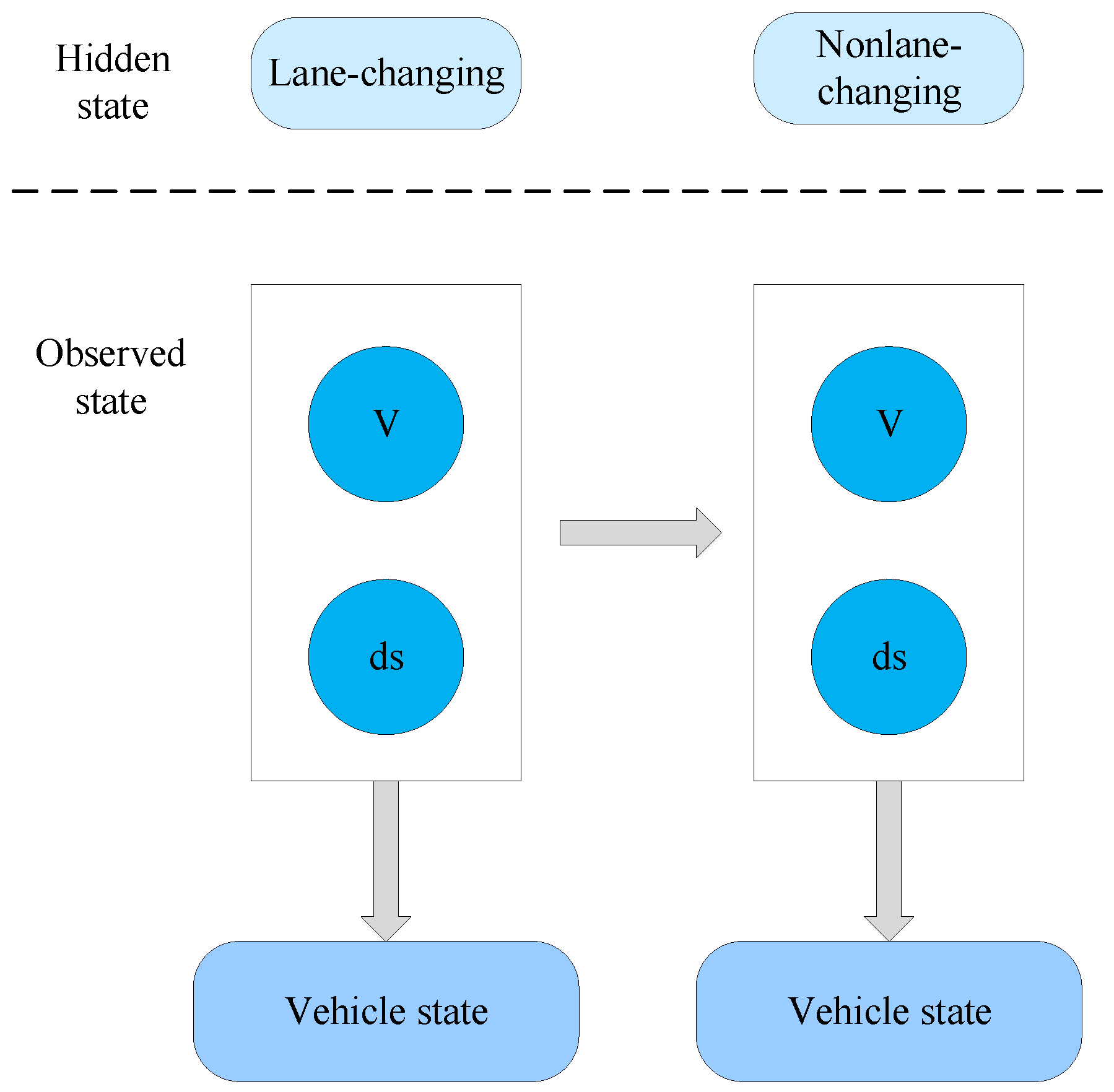
During the lane-changing process, the driving intention exhibited by the driver is an unobservable hidden state, which could be either a lane-changing state or a non-lane-changing state. This intention can be reflected through observable outputs, such as vehicle speed. For example, as shown in Figure 2, $v\left(t\right)$ represents the observable vehicle speed, and $ds\left(t\right)$ represents the driving style exhibited by the driver.

Figure 2. A diagram of lane-changing statuses.

Therefore, the information vector for the lane-changing behavior of connected and autonomous vehicles based on GMMHMM can be expressed as $\lambda =(\pi ,$A$,c,\mu ,U)$, where the following apply:

(1) The hidden state sequence $I=i_1,i_2,\cdots ,i_T$ corresponds to the sequence of observations for a sample vehicle. Each hidden state $i_t$ is drawn from a finite set of two states $S=(s_1,s_2)$, where $s_1$ represents the lane-changing state and $s_2$ represents the non-lane-changing state.

(2) The observation sequence $O=o_1,o_2,\cdots ,o_T$ consists of the observed values of the vehicle operation samples within the observation interval. Here, $o_T$ represents the two-dimensional vehicle operation feature vector observed at time T, where one dimension is the vehicle-related factor $v\left(t\right)$ and the other dimension is the driving style $ds\left(t\right)$, which represents the driver/passenger factor. Thus, the corresponding observation sequence is

$$O\left(t\right)=\left\{v\right(t),ds(t\left)\right\}.$$

(3) The state transition probability matrix $\mathbf{A}$ is defined as $\mathbf{A}=a_{ij}=P(S_{t+1}=q_j|S_t=q_i)$, where $a_{ij}$ represents the probability of transitioning from driving state i to driving state j and $i,j=1,2,\cdots ,N$. The transition probabilities between different vehicle operation states form the state transition probability matrix $\mathbf{A}$.

(4) The random distribution function of the state output events $\mathbf{B}$ is defined as follows:

$$P(o_t=v|q_t=S_j)=\sum _{m=1}^M{c}_{jm}N({\mu }_{jm},U_{jm}).$$

Here, $N({\mu }_{jm},U_{jm})$ is the multivariate Gaussian density function for the output values under vehicle operation state j, where ${\mu }_{jm}$ is the mean vector, $U_{jm}$ is the covariance matrix, and $c_{jm}$ is the Gaussian mixture weight.

(5) The initial state distribution $\pi =[{\pi }_1,{\pi }_2]$, where ${\pi }_1$ represents the probability that the vehicle’s initial hidden state is the lane-changing state, and ${\pi }_2$ represents the probability that the vehicle’s initial hidden state is the non-lane-changing state.

2.3. Lane-Changing Behavior Decision Model of Vehicles

2.3.1. Parameter Estimation of the Lane-Changing Behavior Decision Model

After determining the initial parameters $\lambda$ for the lane-changing behavior information, parameter re-estimation is necessary to optimize the decision performance of the lane-changing decision model. The principle is to maximize $P\left(O\right|\lambda )$ for a given observation sequence $O\left(t\right)=\left\{v\right(t),ds(t\left)\right\}$, thereby obtaining the optimal model parameters $\overline{\lambda }$.

Assuming O is the observation sequence data during the model training process, the unknown driving state sequence data becomes the hidden data item I. Therefore, the lane-changing decision model is a probabilistic model with hidden variables. The problem then transforms into finding the parameter values $\overline{\lambda }$ that maximize $argmaxP\left(O\right|\lambda )$.

The log-likelihood function for all observation data is $logP\left(O\right|\lambda )$, where O represents all observation data $O=(o_1,o_2,\cdots ,o_T)$, and all hidden data are $I=(i_1,i_2,\cdots ,i_T)$. The expectation function of $logP\left(O\right|\lambda )$ concerning the conditional probability distribution $P(I,O|\lambda )$ of the unknown driving state sequence data I given the observed data O and the initial lane-changing model parameters $\lambda$ is

$$Q(\lambda ,\overline{\lambda })=\sum _{I}logP(O,I|\lambda )P(O,I|\overline{\lambda }).$$

(11)

Given that $P(O,I|\lambda )={\pi }_{i_1}{b}_{i_1}\left(o_1\right)a_{i_1{i}_2}{b}_{i_2}\left(o_2\right)a_{i_2{i}_3}\cdots a_{i_{T-1}{i}_T}{b}_{i_T}\left(o_T\right)$, the expanded form of Equation (11) is

$$\begin{array}{cc}\hfill Q(\lambda ,\overline{\lambda })=& \sum _{I}log{\pi }_{i_1}P(O,I|\overline{\lambda })+\sum _I\left(\sum _{t=1}^{T-1}log{a}_{i_t{i}_{t+1}}\right)P\left(O\right|I,\overline{\lambda })\hfill \\ & +\sum _I\left(\sum _{t=1}^{T}log{b}_{i_t}\left(o_t\right)\right)P\left(O\right|I,\overline{\lambda }).\hfill \end{array}$$

(12)

At this point, to obtain the re-estimated parameters $\overline{\lambda }$ for the lane-changing decision model, it is necessary to maximize the function $Q\left(\lambda \right|\overline{\lambda })$.

Since the parameters that need to be maximized in Equation (12) appear separately in three terms, we only need to maximize each term individually [34,35]. Following this, we then optimized each item in three separate steps.

Step 1: Maximize the first term in the expanded form of $Q\left(\lambda \right|\overline{\lambda })$.

$$\begin{array}{c}\hfill \sum _{I}log{\pi }_{i_1}P(O,I|\overline{\lambda })=\sum _{i=1}^{N}log{\pi }_{i}P(O,i_1=i|\overline{\lambda }).\end{array}$$

(13)

Noting that ${\pi }_i$ in Equation (13) satisfies the constraint ${\sum }_{i=1}^N{\pi }_i=1$; thus, we can use the method of Lagrange multipliers. The Lagrangian function is given by the following:

$$\begin{array}{c}\hfill \sum _{i=1}^{N}log{\pi }_{i}P(O,i_1=i|\overline{\lambda })+\gamma \left(\sum _{i=1}^N{\pi }_i-1\right).\end{array}$$

(14)

Taking the partial derivative of Equation (14) with respect to ${\pi }_i$ and setting it to zero, we obtain

$$\begin{array}{c}\hfill {\displaystyle \frac{\partial }{\partial {\pi }_i}}\left[\sum _{i=1}^{N}log{\pi }_{i}P(O,i_1=i|\overline{\lambda })+\gamma \left(\sum _{i=1}^N{\pi }_i-1\right)\right]=0.\end{array}$$

(15)

At this point, introduce the variable ${\gamma }_t\left(i\right)$, which represents the probability of driving intention i at time t. Thus, we have

$$\begin{array}{c}\hfill {\gamma }_t\left(i\right)={\displaystyle \frac{{\alpha }_t\left(i\right){\beta }_t\left(i\right)}{P\left(O\right|\lambda )}}={\displaystyle \frac{{\alpha }_t\left(i\right){\beta }_t\left(i\right)}{{\sum }_{i=1}^N{\alpha }_t\left(i\right){\beta }_t\left(i\right)}},i=1,2,\cdots ,N,t=1,2,\cdots ,T,\end{array}$$

(16)

where ${\alpha }_t\left(i\right)$ represents the probability of observing all driving behaviors up to time t given the driving intention i at time t, and ${\beta }_t\left(i\right)$ represents the probability of observing all driving behaviors after time t given the driving intention i at time t. Therefore, we obtain

$$\widehat{\pi }={\gamma }_t\left(i\right).$$

(17)

Step 2: Maximize the second term in Equation (12):

$$\begin{array}{c}\hfill \sum _I\left(\sum _{t=1}^{T-1}log{a}_{i_t{i}_{t+1}}\right)P\left(O\right|I,\overline{\lambda })=\sum _{i=1}^N\sum _{j=1}^N\sum _{t=1}^{T-1}log{a}_{ij}P(O,i_t=i,i_{t+1}=j|\overline{\lambda }).\end{array}$$

(18)

Since $a_{ij}$ satisfies the constraint ${\sum }_{i=1}^N{\sum }_{j=1}^N{a}_{ij}=1$, we used the method of Lagrange multipliers. The Lagrangian function is given by

$$\begin{array}{c}\hfill \sum _{i=1}^N\sum _{j=1}^N\sum _{t=1}^{T-1}log{a}_{ij}P(O,i_t=i,i_{t+1}=j|\overline{\lambda })+\gamma \left(\sum _{i=1}^N\sum _{j=1}^N{a}_{ij}-1\right).\end{array}$$

(19)

Taking the partial derivative of Equation (19) with respect to $a_{ij}$ and setting it to zero, we obtain

$$\widehat{a_{ij}}={\displaystyle \frac{{\sum }_{t=1}^{T-1}{\epsilon }_t(i,j)}{{\sum }_{t=1}^{T-1}{\gamma }_t\left(i\right)}}.$$

(20)

Let the variable ${\epsilon }_t(i,j)$ represent the probability that, given $\lambda$ and O, the driving intention at time t is $s_i$ and transitions to $s_j$ at time $t+1$. Therefore, we have

$$\begin{array}{cc}\hfill {\epsilon }_t(i,j)& =P(i_t=s_i,i_{t+1}=s_j|O,\lambda )\hfill \\ \hfill & ={\displaystyle \frac{P(i_t=s_i,i_{t+1}=s_j|O,\lambda )}{P\left(O\right|\lambda )}}\hfill \\ \hfill & ={\displaystyle \frac{{\alpha }_t\left(i\right)a_{ij}{b}_j\left(o_{t+1}\right){\beta }_{t+1}\left(j\right)}{{\sum }_{i=1}^N{\alpha }_t\left(i\right){\beta }_t\left(i\right)}}\hfill \\ \hfill & ={\displaystyle \frac{{\alpha }_t\left(i\right)a_{ij}{b}_j\left(o_{t+1}\right){\beta }_{t+1}\left(j\right)}{{\sum }_{i=1}^N{\sum }_{j=1}^N{\alpha }_t\left(i\right)a_{ij}{b}_j\left(o_{t+1}\right){\beta }_{t+1}\left(j\right)}},i=1,2,\cdots ,N,j=1,2,\cdots ,N.\hfill \end{array}$$

(21)

According to Equations (16) and (21), it is easy to see that there is the following relationship between ${\gamma }_t\left(i\right)$ and ${\epsilon }_t(i,j)$:

$${\gamma }_t\left(i\right)=\sum _{j=1}^N{\epsilon }_t(i,j).$$

(22)

Step 3: Maximize the third term in Equation (12):

$$\begin{array}{c}\hfill \sum _I\left(\sum _{t=1}^{T}log{b}_{i_t}\left(o_t\right)\right)P\left(O\right|I,\overline{\lambda })=\sum _{j=1}^N\sum _{t=1}^{T}log{b}_j\left(o_t\right)P(O,i_t=j|\overline{\lambda }),\end{array}$$

(23)

where $b_j\left(o_t\right)$ satisfies the constraint ${\sum }_{j=1}^N{\sum }_{t=1}^T{b}_j\left(o_t\right)=1$. Therefore, we use the method of Lagrange multipliers, and the Lagrangian function is given by

$$\begin{array}{c}\hfill \sum _{j=1}^N\sum _{t=1}^{T}log{b}_j\left(o_t\right)P(O,i_t=j|\overline{\lambda })+\gamma \left(\sum _{j=1}^N\sum _{t=1}^T{b}_j\left(o_t\right)-1\right).\end{array}$$

(24)

Taking the partial derivative of Equation (24) and setting it to zero, we have

$$\widehat{b_j\left(k\right)}={\displaystyle \frac{{\sum }_{t=1,s.t{o}_t=v_k}^T{\gamma }_t\left(j\right)}{{\sum }_{t=1}^T{\gamma }_t\left(j\right)}}.$$

(25)

Here, $\widehat{a_{ij}}$ represents the estimated probability of transitioning from driving intention i to driving intention j, $\widehat{b_j\left(k\right)}$ represents the estimated probability of observing driving behavior k given driving intention j, $\widehat{\pi }$ is the estimated probability distribution of the initial lane-changing intention, and ${\gamma }_t\left(i\right)$ represents the probability of the complete driving observation sequence given the driving intention at time t. Since $\widehat{b_j\left(k\right)}={\sum }_{m=1}^M{c}_{jm}N(o_t,{\mu }_{jm},U_{jm})$, we obtain

$$\left\{\begin{array}{c}{\widehat{c}}_{jm}={\displaystyle \frac{{\sum }_{t=1}^T{\gamma }_t(j,m)}{{\sum }_{t=1}^T{\sum }_{m=1}^M{\gamma }_t(j,m)}},\hfill \\ {\widehat{\mu }}_{jm}={\displaystyle \frac{{\sum }_{t=1}^T{\gamma }_t(j,m)·o_t}{{\sum }_{t=1}^T{\gamma }_t(j,m)}},\hfill \\ {\widehat{U}}_{jm}={\displaystyle \frac{{\sum }_{t=1}^T{\gamma }_t(j,m)·(o_t-{\mu }_{im})(o_t-{\mu }_{jm})}{{\sum }_{t=1}^T{\gamma }_t(j,m)}}.\hfill \end{array}\right.$$

(26)

In summary, the parameters after revaluation can be obtained $\overline{\lambda }=(\widehat{\pi },\widehat{\mathbf{A}},\widehat{c},\widehat{\mu },\widehat{U})$.

2.3.2. Decision Making in Lane-Changing Behavior

Given a set of vehicle observation sequences $O\left(t\right)=\left\{v\right(t),ds(t\left)\right\}$, calculate the probabilities $P\left(O\right|\overline{{\lambda }_C})$ and $P\left(O\right|\overline{{\lambda }_K})$ under the lane-changing model LC-HMM and the lane-keeping model LK-HMM, respectively. Here, $\overline{{\lambda }_C}$ and $\overline{{\lambda }_K}$ are the optimized parameters, which are obtained by re-estimating the lane-changing behavior information vector parameters, as described in Section 2.3.1.

(1)

LC-HMM

Let us calculate the probability $P\left(O\right|\overline{{\lambda }_C})$ for a given set of vehicle observation sequences O under the lane-changing model LC-HMM. Assume the variable ${\alpha }_t\left(i\right)$ represents the probability of observing all previous driving behaviors up to time t given the driving intention i at time t. Thus, we have

$${\alpha }_t\left(i\right)=P(o_1,o_2,\cdots ,o_t,i_t=s_i|\overline{{\lambda }_C}).$$

(27)

Because ${\alpha }_T\left(i\right)=P(o_1,o_2,\cdots ,o_T,i_T=s_i|\overline{\lambda })$, there is

$$\begin{array}{cc}\hfill & {\alpha }_T\left(1\right)+{\alpha }_T\left(2\right)+\cdots +{\alpha }_T\left(N\right)\hfill \\ \hfill & =P(o_1,o_2,\cdots ,o_T,i_T=s_1|\overline{\lambda })+\cdots +P(o_1,o_2,\cdots ,o_T,i_T=s_N|\overline{\lambda })\hfill \\ \hfill & =P(o_1,o_2,\cdots ,o_T|\overline{\lambda })\hfill \\ \hfill & =P\left(O\right|\overline{\lambda }).\hfill \end{array}$$

(28)

Thus, we obtain $P\left(O\right|\overline{{\lambda }_C})={\sum }_{i=1}^N{\alpha }_T\left(i\right)={\sum }_{t=1}^{T-1}{\sum }_{i=1}^N{\alpha }_t\left(i\right)$. To determine $P\left(O\right|\overline{{\lambda }_C})$, we only need to derive the recursive formula for ${\alpha }_t\left(i\right)$.

Given the LC-HMM parameters $\overline{{\lambda }_C}$ and the observation sequence O, the joint probability of the lane-change state $i_1=q_i$ and the observation sequence $o_1$ at the initial time $t=1$ is

$$\begin{array}{cc}\hfill {\alpha }_1\left(i\right)& =P(o_1,i_1=s_i|\lambda )\hfill \\ \hfill & =P\left(o_1\right|i_1=s_i,\lambda )P(i_1=s_i|\lambda )\hfill \\ \hfill & ={\pi }_i{b}_i\left(o_1\right).\hfill \end{array}$$

(29)

Hence, it can be obtained by the recurrence formula

$$\begin{array}{cc}\hfill {\alpha }_t\left(i\right)& =P(o_1,o_2,\cdots ,o_t,i_t=s_i)\hfill \\ \hfill & =P(o_1,o_2,\cdots ,o_{t-1},i_t=s_i)·P\left(o_t\right|o_1,o_2,\cdots ,o_{t-1},i_t=s_i)\hfill \\ \hfill & =P(o_1,o_2,\cdots ,o_{t-1},i_t=s_i)·P\left(o_t\right|i_t=s_i)\hfill \\ \hfill & =\left[\sum _{j=1}^{N}P(o_1,o_2,\cdots ,o_{t-1},i_{t-1}=s_j,i_t=s_i)\right]·P\left(o_t\right|i_t=s_i)\hfill \\ \hfill & =\left[\sum _{j=1}^{N}P(o_1,o_2,\cdots ,o_{t-1},i_{t-1}=s_j)·P(i_t=s_i|i_{t-1}=s_j)\right]·P\left(o_t\right|i_t=s_i)\hfill \\ \hfill & =\left[\sum _{j=1}^N{\alpha }_{t-1}\left(j\right)a_{ij}\right]b_i\left(o_t\right).\hfill \end{array}$$

(30)

Therefore, the forward probability of observing $o_1,o_2,\cdots ,o_t,o_{t+1}$ at time $t+1$ and being in the driving state $s_i$ at $t+1$ is

$${\alpha }_{t+1}\left(i\right)=\left[\sum _{i=1}^N{\alpha }_t\left(i\right)a_{ij}\right]b_i\left(o_{t+1}\right),$$

(31)

where $a_{ij}$ represents the probability of transitioning from driving intention i to driving intention j, $b_i\left(o_{t+1}\right)$ represents the probability of the observation sequence O given the driving intention i, and ${\alpha }_t\left(i\right)$ represents the probability of observing $o_1,o_2,\cdots ,o_t$ and being in driving state $s_i$ at time t. Therefore, ${\alpha }_t\left(i\right)a_{ij}$ is the joint probability of observing $o_1,o_2,\cdots ,o_t$ at time t, being in driving state $s_i$ at time t and transitioning to driving state $s_j$ at time $t+1$. If so, then we can obtain

$$P\left(O\right|\overline{{\lambda }_C})=\sum _{t=1}^{T-1}\sum _{i=1}^N{\alpha }_t\left(i\right)=\sum _{t=1}^{T-1}\sum _{i=1}^N\left[\sum _{j=1}^N{\alpha }_t\left(j\right)a_{ij}\right]b_i\left(o_t\right).$$

(32)

(2)

LK-HMM

When calculating the probability $P\left(O\right|\overline{{\lambda }_K})$ of a given set of vehicle observation sequences O under the lane-keeping model LK-HMM, then the specific derivation process is the same as (1). As such, the following is also true:

$$P\left(O\right|\overline{{\lambda }_K})=\sum _{t=1}^{T-1}\sum _{i=1}^N{\alpha }_t\left(i\right)=\sum _{t=1}^{T-1}\sum _{i=1}^N\left[\sum _{j=1}^N{\alpha }_t\left(j\right)a_{ij}\right]b_i\left(o_t\right).$$

(33)

Finally, compare $P\left(O\right|\overline{{\lambda }_C}$ and $P\left(O\right|\overline{{\lambda }_K})$, where the larger value $max\left\{P\left(O\right|\overline{{\lambda }_C},P\left(O\right|\overline{{\lambda }_K})\right\}$ determines the final lane-changing decision.

3. Empirical Analysis

3.1. Data Preparation

In order to further illustrate the effectiveness and accuracy of the established model, this study used NGSIM vehicle trajectory data as the dataset to study the vehicle lane-changing decision. NGSIM data are collected by the US Federal Highway Administration in the Next Generation Simulation project. In the process of data collection, high-definition cameras are used to obtain the video data of the vehicle running on the road section, images are processed by video processing software, and then some vehicles’ state information are restored.

This study mainly selected data from the US-101 and I-80 sections for empirical analysis. The NGSIM dataset is composed of 18 columns, which is shown in Table 2.

Table 2. The main description of NGSIM data.

Designation	Description	Unit	Converted Unit
Vehicle_ID	The number of vehicles entering the check section	–	–
Frame_ID	Data frame number	0.1 s	0.1 s
X_Location	Distance from the locomotive center to the left side of the road	Feet	m
Y_Location	Distance from locomotive center to segment start	Feet	m
V_Length	The length of the body	Feet	m
V_Vel	Instantaneous vehicle velocity	Feet/s	m/s
V_Acc	Instantaneous acceleration of the vehicle	Feet/s2	m/s
Lane_ID	The lane of vehicle at some point	–	–

Schematic diagrams of the US-101 and I-80 sections are shown in Figure 3.

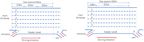
Figure 3. Diagrams of lane-changing statuses.

To ensure the accuracy of the empirical results, the data screening process was conducted as follows:

(1)

To ensure that the vehicles are being driven with the lane-changing behavior characteristics being recorded, the lane ID of the selected vehicles would need to change, and the impact of the on-ramp on lane-changing behavior should be excluded.

(2)

The vehicle type is only small cars, other types were not considered.

(3)

When vehicle $H_1$ is determined, the position of the vehicles $H_2,H_3$, and $H_4$ can also be determined accordingly.

(4)

The vehicle demonstrating lane-changing behavior is calibrated with 1, while the vehicles without lane-changing behavior are calibrated with 0.

(5)

Excluding data with implementing multiple lane-changing and continuous lane-changing behavior.

After data preprocessing, 732 groups of vehicle track data were selected from the US-101 section, including the sample data of 455 vehicles changing lanes and 277 vehicles not changing lanes. Moreover, 746 groups of samples were screened from the I-80 section, including 466 vehicles changing lanes and 280 vehicles not changing lanes. These selected data were randomly divided into training samples and test samples according to a ratio of 7:3. The former was used for parameter estimation of the IR-Logistic model, and the latter was used for validation. The filtered sample vehicle trajectory data are shown in Table 3 and Table 4.

Table 3. The sample vehicle trajectory data for US-101.

v	$\mathbf{\Delta }{\mathit{v}}_{12}$	$\mathbf{\Delta }{\mathit{v}}_{13}$	$\mathbf{\Delta }{\mathit{v}}_{14}$	${\mathit{D}}_{12}$	${\mathit{D}}_{13}$	${\mathit{D}}_{14}$	Lane-Changing Behavior Status
18.29	2.13	−0.61	0.31	29.48	19.56	16.91	1
15.85	2.13	0.31	3.66	10.36	37.17	33.87	1
7.92	17.68	5.18	15.09	3.35	2.13	1.83	0
12.49	−2.44	−0.91	2.13	17.96	22.66	14.25	1
18.89	37.96	5.55	8.82	0.91	2.44	2.13	0
13.72	2.13	1.52	1.83	16.26	28.05	47.27	1
15.85	65.14	9.29	9.92	3.66	6.09	6.71	0
8.23	1.22	−0.61	−1.52	14.04	12.00	20.13	1
10.93	0.88	1.08	3.04	10.23	15.68	13.79	0
24.08	3.35	2.44	6.71	23.31	77.11	19.09	1

Table 4. The sample vehicle trajectory data for I-80.

v	$\mathbf{\Delta }{\mathit{v}}_{12}$	$\mathbf{\Delta }{\mathit{v}}_{13}$	$\mathbf{\Delta }{\mathit{v}}_{14}$	${\mathit{D}}_{12}$	${\mathit{D}}_{13}$	${\mathit{D}}_{14}$	Lane-Changing Behavior Status
6.72	0.62	0.52	0.98	32.54	12.93	15.51	1
7.38	0.12	5.86	4.33	23.82	7.75	6.37	0
11.99	1.52	1.11	0.73	21.77	23.61	21.51	1
6.19	0.74	0.45	1.27	8.04	7.91	8.24	0
8.21	0.59	−2.46	−2.45	12.05	13.88	5.59	0
13.57	−0.15	4.05	2.67	19.47	22.67	35.91	1
10.05	0.92	1.48	2.76	19.21	13.16	42.26	1
9.11	1.92	−0.04	1.49	63.10	10.06	15.81	0
12.59	0.16	0.43	3.81	18.26	18.22	16.92	1
8.46	3.55	3.33	1.14	49.36	10.28	9.06	0

3.2. Results and Analysis

3.2.1. Parameter Estimation of the Lane-Changing Intention Recognition Model

The parameters of the proposed lane-changing intention recognition model were estimated, and the estimated parameter values stabilized after continuous iterations. The results are shown in Table 5 and Table 6.

Table 5. Parameter estimation of the US-101 section.

Variable	Parameter Estimation
v	0.3009
$\Delta v_{12}$	0.5001
$\Delta v_{13}$	0.68
$\Delta v_{14}$	0.55
$D_{12}$	0.08
$D_{13}$	0.08
$D_{14}$	0.2001
$D_{12}·D_{13}$	−0.0199
$D_{12}·D_{14}$	1.5
Constant	−3.279
Random	2.8529

Table 6. Parameter estimation of the I-80 section.

Variable	Parameter Estimation
v	0.3002
$\Delta v_{12}$	0.3604
$\Delta v_{13}$	0.6797
$\Delta v_{14}$	0.4598
$D_{12}$	0.03
$D_{13}$	0.4
$D_{14}$	0.5001
$D_{12}·D_{13}$	0.7999
$D_{12}·D_{14}$	−1.499
Constant	−0.6002
Random	1.494

For the US-101 section, the lane-changing intention recognition model of the CAVs’ lane-changing intention recognition was

$$\begin{array}{cc}\hfill logit{\displaystyle \frac{{\pi }_i}{1-{\pi }_i}}=& -3.279+0.3009v_1+0.5001\Delta v_{12}+0.68\Delta v_{13}+0.55\Delta v_{14}+0.08D_{12}+0.08D_{13}\hfill \\ \hfill & +0.2001D_{14}-0.0199D_{12}·D_{13}+1.5D_{12}·D_{14}+b_i,\hfill \end{array}$$

where $b_i\sim N(0,2.{8529}^2)$.

For the I-80 section, the lane-changing intention recognition model of the CAVs’ lane-changing intention recognition was

$$\begin{array}{cc}\hfill logit{\displaystyle \frac{{\pi }_i}{1-{\pi }_i}}=& -0.6002+0.3002v_1+0.3604\Delta v_{12}+0.6797\Delta v_{13}+0.4598\Delta v_{14}+0.03D_{12}+0.4\hfill \\ & D_{13}+0.5001D_{14}+0.7999D_{12}·D_{13}-1.499D_{12}·D_{14}+b_i,\hfill \end{array}$$

where $b_i\sim N(0,1.{494}^2)$.

3.2.2. Parameter Estimation of Lane-Changing Intention Recognition Model

Based on the vehicle lane-changing data from the US-101 and I-80 segments selected, the driving styles were classified using the average speed and lateral acceleration indicators. The membership functions corresponding to the three types of driving styles for the average speed were established separately for the US-101 and I-80 segments as follows:

(1) The membership function for the average vehicle speed corresponding to the evaluation set for the conservative driving style is

$$f_{US-101}(x,a,b)=\left\{\begin{array}{cc}1\hfill & x\le 1.2\hfill \\ {\displaystyle \frac{12.5-x}{12.5-1.2}}\hfill & 1.2\le x\le 12.5,\hfill \\ 0\hfill & x\ge 12.5\hfill \end{array}{f}_{I-80}(x,a,b)=\left\{\begin{array}{cc}1\hfill & x\le 3.8\hfill \\ {\displaystyle \frac{12.5-x}{12.5-3.8}}\hfill & 3.8\le x\le 12.5\hfill \\ 0\hfill & x\ge 12.5\hfill \end{array}\right.\right..$$

(2) The membership function for the average vehicle speed corresponding to the evaluation set for the moderate driving style is

$$f_{US-101}(x,a,b)=\left\{\begin{array}{cc}0\hfill & x\le 0,\hfill \\ {\displaystyle \frac{x-0}{6.8-0}}\hfill & 0\le x\le 6.8,\hfill \\ 1\hfill & 6.8\le x\le 16.8,f_{I-80}(x,a,b)\hfill \\ {\displaystyle \frac{20.5-x}{20.5-16.8}}\hfill & 16.8\le x\le 20.5,\hfill \\ 0\hfill & x\ge 20.5.\hfill \end{array}=\left\{\begin{array}{cc}0\hfill & x\le 0,\hfill \\ {\displaystyle \frac{x-0}{6.8-0}}\hfill & 0\le x\le 6.8,\hfill \\ 1\hfill & 6.8\le x\le 18.8\hfill \\ {\displaystyle \frac{23.5-x}{23.5-18.8}}\hfill & 18.8\le x\le 23.5,\hfill \\ 0\hfill & x\ge 23.5.\hfill \end{array}\right.\right.$$

(3) The membership function for the average vehicle speed corresponding to the evaluation set for the aggressive driving style is

$$f_{US-101}(x,a,b)=\left\{\begin{array}{cc}0\hfill & x\le 1.2,\hfill \\ {\displaystyle \frac{x-1.2}{20.5-1.2}}\hfill & 1.2\le x\le 20.5,\hfill \\ 1\hfill & x\ge 20.5.\hfill \end{array}{f}_{I-80}(x,a,b)=\left\{\begin{array}{cc}0\hfill & x\le 3.8,\hfill \\ {\displaystyle \frac{x-3.8}{23.5-3.8}}\hfill & 3.8\le x\le 23.5,\hfill \\ 1\hfill & x\ge 23.5.\hfill \end{array}\right.\right.$$

The membership functions corresponding to the three types of driving styles for the lateral acceleration indicators were established separately for the US-101 and I-80 segments as follows:

(1) The membership function corresponding to the lateral acceleration evaluation set for the conservative driving style is

$$f_{US-101}(x,a,b)=\left\{\begin{array}{cc}1\hfill & x\le 0.23,\hfill \\ {\displaystyle \frac{0.78-x}{0.78-0.23}}\hfill & 0.23\le x\le 0.78,\hfill \\ 0\hfill & x\ge 0.78.\hfill \end{array}{f}_{I-80}(x,a,b)=\left\{\begin{array}{cc}1\hfill & x\le 0.23,\hfill \\ {\displaystyle \frac{0.78-x}{0.78-0.23}}\hfill & 0.23\le x\le 0.78,\hfill \\ 0\hfill & x\ge 0.78.\hfill \end{array}\right.\right.$$

(2) The membership function corresponding to the lateral acceleration evaluation set for the moderate driving style is

$$f_{US-101}(x,a,b)=\left\{\begin{array}{cc}0\hfill & x\le 0,\hfill \\ {\displaystyle \frac{x-0}{0.38-0}}\hfill & 0\le x\le 0.38,\hfill \\ 1\hfill & 0.38\le x\le 0.85,\hfill \\ {\displaystyle \frac{1.02-x}{1.02-0.85}}\hfill & 0.85\le x\le 1.02,\hfill \\ 0\hfill & x\ge 1.02.\hfill \end{array}{f}_{I-80}(x,a,b)=\left\{\begin{array}{cc}0\hfill & x\le 0,\hfill \\ {\displaystyle \frac{x-0}{0.38-0}}\hfill & 0\le x\le 0.38,\hfill \\ 1\hfill & 0.38\le x\le 0.85,\hfill \\ {\displaystyle \frac{1.02-x}{1.02-0.85}}\hfill & 0.85\le x\le 1.02,\hfill \\ 0\hfill & x\ge 1.02.\hfill \end{array}\right.\right.$$

(3) The membership function corresponding to the lateral acceleration evaluation set for the aggressive driving style is

$$f_{US-101}(x,a,b)=\left\{\begin{array}{cc}0\hfill & x\le 0.23,\hfill \\ {\displaystyle \frac{x-0.23}{1.02-0.23}}\hfill & 0.23\le x\le 1.02,\hfill \\ 1\hfill & x\ge 1.02.\hfill \end{array}{f}_{I-80}(x,a,b)=\left\{\begin{array}{cc}0\hfill & x\le 0.23,\hfill \\ {\displaystyle \frac{x-0.23}{1.02-0.23}}\hfill & 0.23\le x\le 1.02,\hfill \\ 1\hfill & x\ge 1.02.\hfill \end{array}\right.\right.$$

In real traffic scenarios, both the average speed and lateral acceleration indicators are influenced by the traffic environment at the time, which can interfere with the characterization of the driver’s driving style. Therefore, based on the analysis in the existing literature, the weight values assigned to these two indicators were $w_1=0.5$ and $w_2=0.5$. Then, according to the maximum membership principle, the final driving style classification results were obtained, as shown in Table 7.

Table 7. Driving style classification.

Vehicle_ID	Driving Style	Vehicle_ID	Driving Style
01	Aggressive driving	09	Moderate driving
02	Conservative driving	10	Moderate driving
03	Aggressive driving	11	Aggressive driving
04	Aggressive driving	12	Moderate driving
05	Moderate driving	13	Moderate driving
06	Aggressive driving	14	Aggressive driving
07	Conservative driving	15	Moderate driving
08	Aggressive driving	16	Conservative driving

Next, the lane-changing probability values $\pi$ derived from the lane-changing intention recognition model were used as initial parameters for the lane-changing behavior decision model. Then, we chose the Gaussian mixture number $m=4.$ The lane-changing behavior decision model was trained, and the resulting model parameters was stored in the model library. The specific parameter results for this are as follows:

The training parameters for the LC-HMM model on the US-101 section are

$$\begin{array}{cc}\hfill & \pi =[1,0],A=\left[\begin{array}{cc}0.987& 0.013\\ 0.033& 0.967\end{array}\right],c=\left[\begin{array}{cccc}0.243& 0.298& 0.157& 0.302\\ 0.136& 0.376& 0.286& 0.202\end{array}\right],\hfill \\ \hfill & \mu =\left[\begin{array}{cccc}[15.1,2.0]& [13.01,2.0]& [15.77,2.0]& [14.26,2.0]\\ [13.75,1.0]& [15.7,1.0]& [15.07,1.0]& [9.87,1.0]\end{array}\right],U=\left[\begin{array}{cc}[14.59,0.001]& [0.001,0.02]\\ [7.84,0.003]& [0.003,0.02]\end{array}\right].\hfill \end{array}$$

The training parameters for the LK-HMM model under US-101 are

$$\begin{array}{cc}\hfill & \pi =[0,1],A=\left[\begin{array}{cc}0.977& 0.023\\ 0.002& 0.98\end{array}\right],c=\left[\begin{array}{cccc}0.26& 0.344& 0.06& 0.335\\ 0.062& 0.348& 0.129& 0.46\end{array}\right],\hfill \\ \hfill & \mu =\left[\begin{array}{cccc}[12.5,1.0]& [11.4,1.0]& [12.9,1.0]& [12.12,1.0]\\ [0.71,0.001]& [13.23,2.0]& [5.56,2.0]& [13.81,2.0]\end{array}\right],U=\left[\begin{array}{cc}[8.94,-0.068]& [-0.068,0.056]\\ [8.22,0.001]& [0.001,0.02]\end{array}\right].\hfill \end{array}$$

The training parameters for the LC-HMM model on the I-80 section are

$$\begin{array}{cc}\hfill & \pi =[1,0],A=\left[\begin{array}{cc}0.95& 0.05\\ 0.043& 0.957\end{array}\right],c=\left[\begin{array}{cccc}0.226& 0.366& 0.239& 0.169\\ 0.697& 0.036& 0.238& 0.029\end{array}\right],\hfill \\ \hfill & \mu =\left[\begin{array}{cccc}[8.19,0.97]& [5.58,0.72]& [8.63,0.97]& [7.86,0.96]\\ [7.64,2.0]& [19.38,2.0]& [8.38,2.0]& [20.38,2.0]\end{array}\right],U=\left[\begin{array}{cc}[6.64,0.25]& [0.25,0.09]\\ [7.03,0.003]& [0.003,0.02]\end{array}\right].\hfill \end{array}$$

The training parameters for the LK-HMM model under I-80 are

$$\begin{array}{cc}\hfill & \pi =[0,1],A=\left[\begin{array}{cc}0.921& 0.079\\ 0.018& 0.982\end{array}\right],c=\left[\begin{array}{cccc}0.000238& 0.97& 0.0248& 0.00489\\ 0.000316& 0.0956& 0.809& 0.0947\end{array}\right],\hfill \\ \hfill & \mu =\left[\begin{array}{cccc}[21.3,0]& [3.8,0]& [21.3,0]& [2.53,1.0]\\ [7.3,2.0]& [18.67,2.0]& [8.16,1.0]& [7.39,2.0]\end{array}\right],U=\left[\begin{array}{cc}[5.9,0.001]& [0.001,0.01]\\ [11.64,0.001]& [0.001,0.002]\end{array}\right].\hfill \end{array}$$

3.2.3. The Results of the Decision Making in Lane-Changing Behavior

Further, given a set of vehicle observation test samples, we substituted them into both the LC-HMM and LK-HMM models to calculate the probability values. The data in Table 8 and Table 9 show the logarithm of the probabilities calculated for each sample by the two models. According to the principle of selecting the class with the highest conditional probability as the lane-changing decision result, we chose the largest values in each row as the final decision result, which are highlighted in bold. The accuracy rates of the LC-HMM and LK-HMM decision results for the test set data on the US-101 section were $91.41\%$ and $90.3\%$, respectively, and, for the I-80 section, they were $90.33\%$ and $90.6\%$, respectively.

Table 8. Decision results for a single test sample for the US-101 section.

Sample Number	LC-HMM	LK-HMM
1	−1.22	−41.11
2	−5.97	−54.10
3	−115.99	−5.75
4	−114.43	−4.39
5	−10.925	−50.66
6	−4.82	−51.17
7	−4.13	−49.24
8	−10.80	−8.78
9	−2.19	−45.26
10	−116.14	−5.9

Table 9. Decision results for a single test sample for the I-80 section.

Sample Number	LC-HMM	LK-HMM
1	−19.89	−22.63
2	−16.9	−2.18
3	−4.97	−20.26
4	−9.86	−22.67
5	−17.24	−2.53
6	−6.45	−21.93
7	−95.42	53.56
8	−25.45	−120.45
9	−17.83	2.95
10	−33.98	−16.09

4. Conclusions and Discussion

This paper investigated the lane-changing behavior decision making of the vehicles. First, we capitalized on the vehicle-to-vehicle communication capabilities of the vehicles to develop a logistic model that incorporates both interaction and random effects for lane-changing intention recognition. Next, to account for the influence of the driver behavior on lane-changing decisions, we introduced driving styles as an indicator of the driver preferences during lane changes. This driving style was classified into three distinct categories—conservative, moderate, and aggressive—using membership functions. Subsequently, we employed a mixed Gaussian hidden Markov model to construct a lane-changing behavior decision-making model that integrates driving styles. Finally, we conducted empirical analysis using real-world traffic data from the US-101 and I-80 corridors in the NGSIM database. The results demonstrate that our proposed lane-changing behavior decision-making model achieves high accuracy in identifying lane-changing behaviors.

There were some interesting limitations in this study. For example, factors such as communication delays and information transmission errors in the vehicles will increase the uncertainty in vehicle decision-making analysis. These factors were not considered in this model. In the future, we can incorporate these factors to construct a more comprehensive vehicle lane-changing behavior decision-making model.

References

- Bocklisch, F.; Bocklisch, S.F.; Beggiato, M.; Krems, J.F. Adaptive fuzzy pattern classification for the online detection of driver lane change intention. Neurocomputing 2017, 262, 148–158. [Google Scholar] [CrossRef]
- Birrell, S.A.; Wilson, D.; Yang, C.P.; Dhadyalla, G.; Jennings, P. How driver behaviour and parking alignment affects inductive charging systems for electric vehicles. Transp. Res. Part C Emerg. Technol. 2015, 58, 721–731. [Google Scholar] [CrossRef]
- Deng, J.H.; Feng, H.H. A multilane cellular automaton multi-attribute lane-changing decision model. Phys. A Stat. Mech. Its Appl. 2019, 529, 121545. [Google Scholar] [CrossRef]
- Peng, J.; Wang, C.; Fu, R.; Yuan, W. Extraction of parameters for lane change intention based on driver’s gaze transfer characteristics. Saf. Sci. 2020, 126, 104647. [Google Scholar] [CrossRef]
- Xing, Y.; Lv, C.; Wang, H.; Cao, D.; Velenis, E. An ensemble deep learning approach for driver lane change intention inference. Transp. Res. Part C Emerg. Technol. 2020, 115, 102615. [Google Scholar] [CrossRef]
- Wen, J.; Wu, C.; Zhang, R.; Xiao, X.; Nv, N.; Shi, Y. Rear-end collision warning of connected automated vehicles based on a novel stochastic local multivehicle optimal velocity model. Accid. Anal. Prev. 2020, 148, 105800. [Google Scholar] [CrossRef]
- Yang, Z.; Zhang, W.; Feng, J. Predicting multiple types of traffic accident severity with explanations: A multi-task deep learning framework. Saf. Sci. 2022, 146, 105522. [Google Scholar] [CrossRef]
- Cafiso, S.; Pappalardo, G. Safety effectiveness and performance of lane support systems for driving assistance and automation–Experimental test and logistic regression for rare events. Accid. Anal. Prev. 2020, 148, 105791. [Google Scholar] [CrossRef]
- Sharma, O.; Sahoo, N.; Puhan, N.B. Dynamic Planning of Optimally Safe Lane-change Trajectory for Autonomous Driving on Multi-lane Highways Using a Fuzzy Logic–based Collision Estimator. J. Auton. Transp. Syst. 2024, 1, 1–50. [Google Scholar] [CrossRef]
- Wu, F.W.; Fu, R.; Niu, Z.L. Driver’s Fixation Transition Mode during Lane Changing Process. J. Transp. Syst. Eng. Inf. Technol. 2014, 14, 68. [Google Scholar]
- Kauffmann, N.; Winkler, F.; Naujoks, F.; Vollrath, M. “What Makes a Cooperative Driver?” Identifying parameters of implicit and explicit forms of communication in a lane change scenario. Transp. Res. Part Traffic Psychol. Behav. 2018, 58, 1031–1042. [Google Scholar] [CrossRef]
- Du, L.; Chen, W.; Ji, J.; Pei, Z.; Tong, B.; Zheng, H. A Novel Intelligent Approach to Lane-Change Behavior Prediction for Intelligent and Connected Vehicles. Comput. Intell. Neurosci. 2022, 2022, 9516218. [Google Scholar] [CrossRef] [PubMed]
- Wang, W.; Qie, T.; Yang, C.; Liu, W.; Xiang, C.; Huang, K. An Intelligent Lane-Changing Behavior Prediction and Decision-Making Strategy for an Autonomous Vehicle. IEEE Trans. Ind. Electron. 2022, 69, 2927–2937. [Google Scholar] [CrossRef]
- Ali, Y.; Hussain, F.; Bliemer, M.C.; Zheng, Z.; Haque, M.M. Predicting and explaining lane-changing behaviour using machine learning: A comparative study. Transp. Res. Part C Emerg. Technol. 2022, 145, 103931. [Google Scholar] [CrossRef]
- Hu, X.; Chen, S.; Zhao, J.; Wang, R.; Liu, W. Risk identification and prediction model for continuous-lane-change vehicles considering driving style. Expert Syst. Appl. 2025, 259, 125292. [Google Scholar] [CrossRef]
- Xu, T.; Zhang, Z.; Wu, X.; Qi, L.; Han, Y. Recognition of lane-changing behaviour with machine learning methods at freeway off-ramps. Phys. A Stat. Mech. Its Appl. 2021, 567, 125691. [Google Scholar] [CrossRef]
- David, R.; Rothe, S.; Soffker, D. Lane changing behavior recognition based on Artificial Neural Network-based State Machine approach. In Proceedings of the 2021 IEEE International Intelligent Transportation Systems Conference (ITSC), Indianapolis, IN, USA, 19–22 September 2021; pp. 3444–3449. [Google Scholar]
- Gipps, P.G. A model for the structure of lane-changing decisions. Transp. Res. B Part Methodol. 1986, 20, 403–414. [Google Scholar] [CrossRef]
- Schakel, W.J.; Knoop, V.L.; Van Arem, B. Integrated lane change model with relaxation and synchronization. Transp. Res. Rec. 2012, 2316, 47–57. [Google Scholar] [CrossRef]
- Ulbrich, S.; Maurer, M. Probabilistic online POMDP decision making for lane changes in fully automated driving. In Proceedings of the 16th International IEEE Conference on Intelligent Transportation Systems (ITSC 2013), Hague, The Netherlands, 6–9 October 2013; pp. 2063–2067. [Google Scholar]
- Li, K.; Wang, X.; Xu, Y.; Wang, J. Lane changing intention recognition based on speech recognition models. Transp. Res. Part C Emerg. Technol. 2016, 69, 497–514. [Google Scholar] [CrossRef]
- Jia, S.; Hui, F.; Wei, C.; Zhao, X.; Liu, J. Lane-Changing Behavior Prediction Based on Game Theory and Deep Learning. J. Adv. Transp. 2021, 2021, 6634960. [Google Scholar] [CrossRef]
- Xia, Y.; Qu, Z.; Sun, Z.; Li, Z. A human-like model to understand surrounding vehicles’ lane changing intentions for autonomous driving. IEEE Trans. Veh. Technol. 2021, 70, 4178–4189. [Google Scholar] [CrossRef]
- Yu, K.; Lin, L.; Alazab, M.; Tan, L.; Gu, B. Deep learning-based traffic safety solution for a mixture of autonomous and manual vehicles in a 5G-enabled intelligent transportation system. IEEE Trans. Intell. Transp. Syst. 2021, 22, 4337–4347. [Google Scholar] [CrossRef]
- Khelfa, B.; Ba, I.; Tordeux, A. Predicting highway lane-changing maneuvers: A benchmark analysis of machine and ensemble learning algorithms. Phys. A Stat. Mech. Its Appl. 2023, 612, 128471. [Google Scholar] [CrossRef]
- David, R.; Söffker, D. A review on machine learning-based models for lane-changing behavior prediction and recognition. Front. Future Transp. 2023, 4, 950429. [Google Scholar] [CrossRef]
- Li, Z.; Wang, Y.; Zuo, Z.; Hu, C. A Hierarchical Intention Inference Model for Connected and Automated Vehicles. IEEE Trans. Intell. Veh. 2024. [Google Scholar] [CrossRef]
- Xia, J.; Wu, X.; Wang, Y.; Li, D. Personalized Lane Changing Decision-Making Based On Vehicle Environment Interaction. In Proceedings of the 2024 8th CAA International Conference on Vehicular Control and Intelligence (CVCI), Chongqing, China, 25–27 October 2024; pp. 1–6. [Google Scholar]
- Wang, T.; Ma, M.; Liang, S.; Yang, J.; Wang, Y. Robust lane change decision for autonomous vehicles in mixed traffic: A safety-aware multi-agent adversarial reinforcement learning approach. Transp. Res. Part C Emerg. Technol. 2025, 172, 105005. [Google Scholar] [CrossRef]
- Jin, H.; Duan, C.; Liu, Y.; Lu, P. Gauss mixture hidden Markov model to characterise and model discretionary lane-change behaviours for autonomous vehicles. IET Intell. Transp. Syst. 2020, 14, 401–411. [Google Scholar] [CrossRef]
- Sharma, O.; Sahoo, N.C.; Puhan, N.B. Highway lane-changing prediction using a hierarchical software architecture based on support vector machine and continuous hidden markov model. Int. J. Intell. Transp. Syst. Res. 2022, 20, 519–539. [Google Scholar] [CrossRef]
- Sun, K.; Zhao, X.; Wu, X. A cooperative lane change model for connected and autonomous vehicles on two lanes highway by considering the traffic efficiency on both lanes. Transp. Res. Interdiscip. Perspect. 2021, 9, 100310. [Google Scholar] [CrossRef]
- Wang, Z.; Zhao, X.; Chen, Z.; Li, X. A dynamic cooperative lane-changing model for connected and autonomous vehicles with possible accelerations of a preceding vehicle. Expert Syst. Appl. 2021, 173, 114675. [Google Scholar] [CrossRef]
- Wu, D.; Ma, J. An effective EM algorithm for mixtures of Gaussian processes via the MCMC sampling and approximation. Neurocomputing 2019, 331, 366–374. [Google Scholar] [CrossRef]
- Yang, M.S.; Lai, C.Y.; Lin, C.Y. A robust EM clustering algorithm for Gaussian mixture models. Pattern Recognit. 2012, 45, 3950–3961. [Google Scholar]
Disclaimer/Publisher’s Note: The statements, opinions and data contained in all publications are solely those of the individual author(s) and contributor(s) and not of MDPI and/or the editor(s). MDPI and/or the editor(s) disclaim responsibility for any injury to people or property resulting from any ideas, methods, instructions or products referred to in the content. |
© 2025 by the authors. Licensee MDPI, Basel, Switzerland. This article is an open access article distributed under the terms and conditions of the Creative Commons Attribution (CC BY) license (https://creativecommons.org/licenses/by/4.0/).