Article

A Surrogate-Assisted Gray Prediction Evolution Algorithm for High-Dimensional Expensive Optimization Problems

1
School of Information and Mathematics, Yangtze University, Jingzhou 434023, China
2
School of Information Engineering, Jiaxing Nanhu University, Jiaxing 314001, China
*
Authors to whom correspondence should be addressed.
Mathematics 2025, 13(6), 1007; https://doi.org/10.3390/math13061007
Submission received: 20 February 2025 / Revised: 9 March 2025 / Accepted: 10 March 2025 / Published: 20 March 2025

Abstract

:
Surrogate-assisted evolutionary algorithms (SAEAs), which combine the search capabilities of evolutionary algorithms (EAs) with the predictive capabilities of surrogate models, are effective methods for solving expensive optimization problems (EOPs). However, the over-reliance on the accuracy of the surrogate model causes the optimization performance of most SAEAs to decrease drastically with the increase in dimensionality. To tackle this challenge, this paper proposes a surrogate-assisted gray prediction evolution (SAGPE) algorithm based on gray prediction evolution (GPE). In SAGPE, both the global and local surrogate model are constructed to assist the GPE search alternately. The proposed algorithm improves optimization efficiency by combining the macro-predictive ability of the even gray model in GPE for population update trends and the predictive ability of surrogate models to synergistically guide population searches in promising directions. In addition, an inferior offspring learning strategy is proposed to improve the utilization of population information. The performance of SAGPE is tested on eight common benchmark functions and a speed reducer design problem. The optimization results are compared with existing algorithms and show that SAGPE has significant performance advantages in terms of convergence speed and solution accuracy.

1. Introduction

Evolutionary algorithms (EAs) [1] have received much attention for their ability to provide effective solutions in complex optimization problems. However, the large number of function evaluations required by EAs to find the optimal value makes it expensive or even unacceptable in terms of time cost in solving optimization problems that require time-consuming computer simulations. Computationally expensive optimization problems are commonly referred to as EOPs [2]. To reduce the computational cost of EAs for solving EOPs, researchers have investigated surrogate-assisted evolutionary algorithms (SAEAs) [3]. The basic idea of SAEAs is to reduce computational cost by using surrogate models instead of true fitness evaluation functions and defining prescreening strategies to select individuals from the search population that need to be evaluated with the true function [4]. Polynomial regression (PR) [5], radial basis function (RBF) [6], Kriging model [7], and support vector regression (SVR) [8] are commonly used surrogate models.
Almost all traditional EAs have the potential to solve EOPs with the assistance of surrogate models [9]. In SAEAs, the most commonly used EAs are particle swarm optimization (PSO) [10] and differential evolution (DE) [11], in addition to competitive swarm optimizer (CSO) [12], gray wolf optimization (GWO) [13], and others. Depending on the surrogate model, the existing SAEAs can be broadly categorized into three types, i.e., global-model-assisted EAs [14], local-model-assisted EAs [15], and hybrid-model-assisted EAs [16]. Global surrogate models, which focus on exploring the entire search space, are often used to approximate the entire landscape of a problem. Di Nuovo et al. [17] presented a study on the use of inexpensive fuzzy function approximation models in selecting promising candidates for true function evaluation in multiobjective optimization problems. Li et al. [18] proposed a fast surrogate-assisted particle swarm algorithm (FSAPSO) for medium dimensional problems, which designs a prescreening criterion that considers both the predicted fitness value and the distance. Local surrogate models aim to make accurate predictions within a small search area, focusing on the development of promising search areas. Ong et al. [19] constructed a local RBF model based on the principle of transformational inference and then used a trust domain approach to cross-use the true function and RBF for the objective and constraint functions. Li et al. [20] defined a number of subproblems in each search generation and constructs a local surrogate to optimize each of them. Due to the limited number of training examples available, a single global or local model cannot effectively fit a variety of problem landscapes, making it often difficult for single-model SAEAs to effectively address different EOPs [11]. To balance exploration and exploitation, there is a growing interest in hybrid surrogate models. Hybrid surrogate models typically consist of a global surrogate model and a local surrogate model and have been shown to outperform single surrogate models on most problems. Wang et al. [21] proposed an evolutionary sampling-assisted optimization (ESAO) for high-dimensional EOPs, which performs global and local searches alternately based on whether the current optimal value is improved or not. A surrogate-assisted competitive swarm optimization (SACSO), which uses global search, local search, and dyadic-based search as three different criteria to select suitable particles for true evaluation, was proposed in Pan et al. [22]. A generalized surrogate-assisted DE (GSDE) [23] was proposed to solve the optimal design problem of turbomachinery vane grids. In a GSDE, an RBF is introduced into the population to update the process to achieve a good balance between global and local searches. Recently, Zhang et al. [24] developed a hierarchical surrogate framework for hybrid evolutionary algorithms. In the global search phase, RBF surrogates are used to guide the teaching–learning-based optimization to locate promising subregions. In the local search phase, a new dynamic surrogate set is proposed to assist differential evolution to speed up the convergence process.
All of the above methods have good performance in solving EOPs. The effectiveness of using surrogate models to help EAs reduce the computational costs is demonstrated in them. However, due to the over-reliance on surrogate models, most existing SAEAs still require extensive true function evaluation before finding a high-quality solution. The powerful search capability of traditional EAs lies in the fact that they do not need the gradient information of the objective function and search for the optimal value by means of information interaction through mutation and crossover operations between current or historical individuals [25]. It is well known that surrogate models are the main source of population fitness information in the SAEAs framework. The “curse of dimensionality” makes it difficult to establish accurate surrogate models with limited samples as the dimension of the problem increases. Inaccurate surrogates may provide unreliable fitness information to the search population, mislead the population search, and waste computational resources [13]. Therefore, in the design of SAEAs, how to reduce the risk of inaccurate surrogate models misleading the direction of the population search and efficiently find a good solution is an urgent problem that needs to be solved.
EAs that utilize population prediction information for searches provide a potential opportunity to address the above problem. They use a prediction model as a reproduction operator to predict the next generation of the population based on the iterative information of the historical population. During the optimization process, all individuals search in the promising direction predicted by the prediction model based on the historical iteration information rather than by moving closer to or farther away from specific individuals. This feature can effectively reduce the risk that the search direction of the population is misdirected by inaccurate surrogate models. In addition, the ability of the reproduction operator in EAs designed based on predictive models to predict population renewal trends has the potential to synergize with surrogate models to guide the population search in promising directions, thereby improving the efficiency of finding optimal values. Therefore, EAs that utilize population prediction information for searching have great potential for development in the design of SAEAs.
Gray prediction evolution (GPE) [26] has attracted considerable attention for its excellent performance among EAs that use population prediction information to search. Based on GPE, several improved algorithms with excellent performance have been successfully developed and applied in various fields [27]. The advantage that the even gray model (EGM(1,1)) operator in GPE can make accurate predictions on small sample data makes it very suitable for EOPs with scarce computational resources. Based on the considerations above, a surrogate-assisted method on the basis of the GPE is proposed in this paper. To the best of our knowledge, this study is the first attempt to combine the predictive information of search populations with surrogate models to solve EOPs. The proposed method is called the surrogate-assisted gray prediction evolution (SAGPE) algorithm. In order to balance exploration and exploitation, SAGPE constructs a global RBF model and a local RBF model alternately to assist GPE in the search. During the optimization process, surrogate models are used to predict the fitness values of offspring generated by the GPE reproduction operator, and the individual with the best surrogate model value is selected for true function evaluation. Individuals in the offspring whose model values are better than those of the parental individuals are retained by greedy selection. If the global search does not find a better solution than the current global optimal value, it switches to a local search and vice versa. In addition, greedy selection only retains the individuals with good fitness values in each search of EAs and directly discards the information of individuals with poor fitness values, which results in the loss of information. To improve the use of population information, this paper designed an inferior offspring learning strategy in the global search phase to improve the quality of candidate individuals. Experiments for SAGPE compared with five other SAEAs were conducted on eight commonly used benchmark functions and a real world optimization problem. The experimental results show that SAGPE outperforms other algorithms in terms of optimization effectiveness and convergence speed on most problems.
The main works of this paper are as follows:
A gray prediction technique is introduced to solve expensive optimization problems (EOPs). In this work, an even gray model (EGM(1,1)) operator is adopted in concert with a surrogate model to guide the population to search in a promising direction.
We verified that predictive model operators can be better combined with surrogate models to search for optimal solutions compared to the traditional conventional mutation and crossover operators.
An inferior individual offspring strategy is proposed to improve the quality of candidate individuals used for true function evaluation.
We have proposed a surrogate-assisted gray prediction evolution algorithm (SAGPE) for solving EOPs.
The remainder of this paper is organized as follows. Section 2 describes several relevant technologies. Section 3 explains the details of the proposed SAGPE. Section 4 demonstrates the performance of SAGPE in solving EOPs through numerical experiments. Section 5 is a discussion of future work and includes concluding remarks.

2. Related Techniques

2.1. GPE Algorithm

In this paper, GPE is used as the underlying search algorithm. As a novel population-intelligent optimization algorithm with strong global search capability, GPE takes the results of EGM(1,1) prediction of population updating trends as offspring. Specifically, the prediction of the EGM(1,1) consists of the following three steps: (1) transforming irregular discrete data into a dataset with an exponential growth pattern by data accumulation, (2) constructing an exponential function from the accumulated dataset and then predicting the next element of the transformed dataset, and (3) obtaining the predicted elements of the raw discrete data by backward derivation. The computational flow of EGM(1,1) is described as follows.
Let a raw data sequence exist as X ( 0 ) = ( x ( 0 ) ( 1 ) , x ( 0 ) ( 2 ) , , x ( 0 ) ( n ) ) . The first-order accumulation operation of X ( 0 ) generates the transformed data sequence as follows:
X ( 1 ) = ( x ( 1 ) ( 1 ) , x ( 1 ) ( 2 ) , , x ( 1 ) ( n ) ) ,
where
x ( 1 ) ( k ) = i = 1 k x ( 0 ) ( i ) , k = 1 , 2 , n .
The immediate neighboring mean sequence Z ( 1 ) of X ( 1 ) is generated as follows:
Z ( 1 ) = ( z ( 1 ) ( 2 ) , z ( 1 ) ( 3 ) , , z ( 1 ) ( n ) ) ,
where
z ( 1 ) ( k ) = 0.5 x ( 1 ) ( k ) + 0.5 x ( 1 ) ( k 1 ) , k = 2 , 3 , , n .
We establish the following first-order linear ordinary differential equation for X ( 0 ) as follows:
d x ( 1 ) / d t + α x ( 1 ) = β ,
where α and β are the parameters to be estimated. We then discretize Equation (3) to obtain x ( 0 ) ( k ) + α z ( 1 ) ( k ) = β , k = 2 , 3 , , n , i.e., EGM(1,1). We write this equation in matrix form as Y = B u ^ . Therein,
Y = [ x ( 0 ) ( 2 ) , x ( 0 ) ( 3 ) , , x ( 0 ) ( n ) ] T , B = z ( 1 ) 2 1 z ( 1 ) 3 1 z ( 1 ) n 1 , u ^ = [ α , β ] .
The least squares method is utilized to solve for the parameter u ^ . The following equation is obtained:
[ α , β ] T = [ B T , B ] 1 B T Y .
We obtain the values of α and β . Solving Equation (3) with α and β gives x ( 1 ) ( t ) = ( x ( 1 ) ( 1 ) β / α ) e x p α t + β / α . It is then discredited to obtain the following prediction equation:
x ^ ( 1 ) ( k + 1 ) = ( x ( 0 ) ( 1 ) β / α ) e x p α k + β / α , k = 0 , 1 , , n 1 .
Therein, x ^ ( 1 ) ( k + 1 ) denotes the prediction sequence of the transformed data sequence. Then, the predicted value of the raw sequence is obtained by backward derivation. The specific formula is as follows:
x ^ ( 0 ) ( k + 1 ) = x ^ ( 1 ) ( k + 1 ) x ^ ( 1 ) ( k )
Finally, substituting x ^ ( 1 ) ( k + 1 ) = ( x ( 0 ) ( 1 ) β / α ) e x p α k + β / α and x ^ ( 1 ) ( k ) = ( x ( 0 ) ( 1 ) β / α ) e x p α ( k 1 ) + β / α into (6) gives the following equation:
x ^ ( 0 ) ( k + 1 ) = ( x ( 0 ) ( 1 ) β / α ) ( 1 e x p α ) e x p α k , k = 1 , 2 , , n 1 .
Note that the GPE requires information from three generations of populations for the next generation of population prediction. Therefore, it is necessary to randomly generate three populations in the initialization phase and perform selection operations on the offspring by using the third-generation population as the parent in all subsequent searches. In addition, an exponential function cannot be constructed for the EGM(1,1) prediction when two identical data exist. Therefore, to facilitate the population search, the GPE generates offspring during the search according to the following rules:
(i)
If the maximum Euclidean distance between three individuals in the data sequence is less than a given threshold η , the GPE generate offspring by random perturbation.
(ii)
If the distance between any two values of the sequence is less than a given threshold η , it uses linear fitting to generate offspring.
(iii)
Otherwise, it uses EGM(1,1) to generate offspring.
Ref. [26] is provided for readers interested in detailed information on GPE.

2.2. RBF Model

The RBF [28] is a commonly used surrogate model, and studies have shown that the RBF performs well on both low-dimensional and high-dimensional problems [29]; additionally, the time of modeling the RBF does not rise significantly with the increase in dimension [9]. In this study, the RBF is used to build a surrogate model to assist in the GPE search.
Let x 1 , x 2 , , x n and f ( x 1 ) , f ( x 2 ) , , f ( x n ) denote n input points in N-dimensional space and their corresponding output values in output space, respectively. The definition formula of the RBF is
f ^ ( x ) = i = 1 n ω i φ ( x x i ) + p ( x ) ,
in which f ^ ( x ) denotes the function value obtained by RBF interpolation fitting, ω i denotes the weight coefficient, and φ ( · ) denotes kernel function. In this paper, the cubic function represented by φ ( r ) = r 3 serves as the kernel function. · denotes the Euclidean distance between c and c i , that is, the input points and the centroid. p ( x ) is a linear function. For the unknown parameter ω = ( ω 1 , ω 2 , , ω n ) T , it can be obtained by the solution of the equation below:
Φ P P T 0 w b = F 0 ,
where Φ is the n × n matrix having elements Φ i j = φ ( x i x j ) , i , j = 1 , 2 , , n . P is the kernel function matrix of the linear function p ( x ) . b = ( b 1 , b 2 , b D + 1 ) T is the vector of coefficients for p ( x ) , and F = ( f ( x 1 ) , f ( x 2 ) , , f ( x n ) ) T . If rank (P) = D + 1, then the matrix Φ P P T 0 is non-singular. Then, the system has a unique solution. In other words, the RBF model can be uniquely determined.

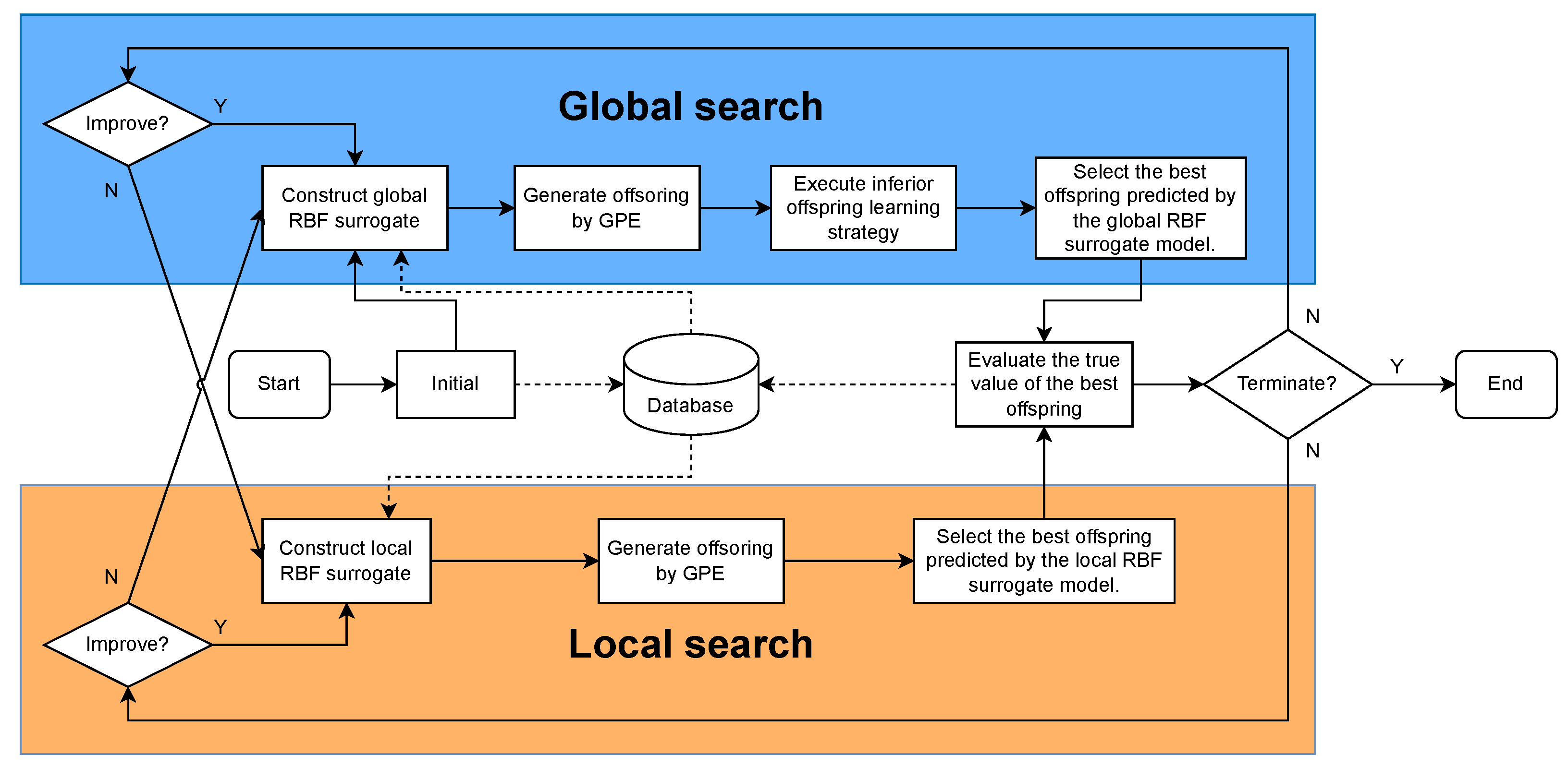
3. Surrogate-Assisted Gray Prediction Evolution Algorithm

The use of predictive information from populations as offspring makes SAGPE different from other SAEAs. The framework and main components of SAGPE are described in detail as follows.

3.1. Overall Framework

Through the predictive search capabilities of GPE as well as the prediction ability for populations’ true fitness values of RBF models, SAGPE is able to efficiently find good solutions. SAGPE searches for optimal solutions by alternately performing global and local searches. Both search components include GPE and an RBF surrogate model. The surrogate model in the global search is constructed based on all existing samples in the database. The best τ fitness values in the current database are used to construct the surrogate model for local search. The main framework of SAGPE is shown in Figure 1, and the solid and dashed lines in it represent the operation flow and data flow of the algorithm, respectively. Initial samples are generated by means of Latin Hypercube Sampling (LHS) [30]. All samples obtained by LHS are evaluated by true function value and added to the database as the initial dataset for training surrogate models. Since three generations of populations are required for the reproduction operation of the GPE, this paper obtained three populations by performing three random samples during the initialization population stage and used the third population as the parent population. After initialization, SAGPE starts the optimization process from the global search phase, and the search mode will be changed to local search if it cannot successfully find a solution better than the global optimal value. Similarly, the search mode will be changed from local to global search if it cannot successfully obtain a solution that improves the global optimal value. The search process ends and the optimization results are output when the maximum amount of true function evaluations is exhausted.

3.2. Global Search

The pseudo-code for performing a global search is presented in Algorithm 1. The global RBF model is trained to predict the fitness value of the offspring by using all the samples in the database. The model generates offspring using GPE and predicts fitness values of the offspring using a global RBF model. The offspring with the best model predicted fitness value is selected for true evaluation. The global search continues if the current optimal function value is improved. If no individual is found that is better than the current best sample, the search is switched to a local search. To ensure convergence of the search population, only individuals with better model predictions than their parents are retained in the offspring population. Considering that each search retains only the individual whose predicted fitness values are better than those of the parent, information about the individual whose predicted fitness values are worse than those of the parent is lost. This paper designed an inferior offspring learning strategy for offspring with worse predicted fitness values than their parents for improving the utilization of population information. Specifically, during the global search phase, those individuals in the offspring population whose predicted fitness values have not improved relative to their parents will learn from the current optimal sample. Algorithm 2 gives the pseudo-code for the inferior offspring learning strategy. It should be emphasized that the population should always search in the direction predicted by EGM(1,1), thus fully combining the predictive search capability of EGM(1,1) with the predictive capability of the surrogate model. Therefore, any offspring that has performed an inferior offspring learning strategy will not be retained even if its predicted fitness value exceeds that of the parent.
Algorithm 1 Pseudo-code of the global search
  1:
Input: Current best sample x g b e s t ; Current global optimal value f ( x g b e s t ) ; Database, including sample points and their true function values;
  2:
repeat
  3:
   Construct a global RBF model ( f ^ g ) using all samples;
  4:
   Generate offspring by GPE;
  5:
   Obtain predicted fitness values of offspring using f ^ g ;
  6:
   Preserve offspring with better predicted fitness values than the parent;
  7:
   Run Algorithm 2 to get new offspring;
  8:
   Obtain predicted fitness values of new offspring using f ^ g ;
  9:
   Select the individual with the best prediction of new offspring, x g , and calculate its true function value, f ( x g ) ;
10:
    Store x g and f ( x g ) in the database;
11:
    if  f ( x g ) < f ( x g b e s t )  then
12:
       Replace f ( x g ) with f ( x g b e s t ) as the current global optimal value;
13:
       Replace x g with x g b e s t as the current best sample;
14:
    end if
15:
until Step 11 is false
16:
Output:  x g b e s t , f ( x g b e s t ) ;

3.3. Local Search

Unlike a global surrogate model that focuses on exploration, a local surrogate model is constructed for increasing the searching speed in regions of promise. In SAGPE, the best τ solutions evaluated by true function value are used to construct a local surrogate model for local searching. The offspring is generated by GPE, and then the local RBF model is used to evaluate the offspring. Only individuals in the offspring population with better model predictions than the previous generation are retained. The offspring with the best model-predicted adaptation values are selected for true evaluation. If the function value of a sample added to the database is not better than the current optimal function value, it switches to a global search. The pseudo-code of the local search is noted in Algorithm 3.
Algorithm 2 Pseudo-code of the inferior offspring learning strategy
  1:
Input: Current best sample x b e s t ; Population size P s i z e ;
       Offspring N e w and their predicted fitness values N e w v a l u e ;
       Parent O l d and their predicted fitness values O l d v a l u e .
  2:
Set i = 1;
  3:
while  i < P s i z e   do
  4:
   if  N e w v a l u e ( i ) > O l d v a l u e ( i ) then
  5:
       N e w ( i ) = N e w ( i ) + r a n d ( x b e s t N e w ( i ) ) ;
  6:
   end if
  7:
    i = i + 1 ;
  8:
end while
  9:
Output:  N e w ;
Algorithm 3 Pseudo-code of the local search
  1:
Input: Current best sample x g b e s t ; Current global optimal value f ( x g b e s t ) ; Database, including sample points and their true function values;
  2:
repeat
  3:
   Construct a local RBF model ( f l ^ ) using τ best samples in the database;
  4:
   Generate offspring by GPE;
  5:
   Predicted fitness values for all offspring are obtained by using f l ^ ;
  6:
   Preserve offspring with better predicted fitness values than the parent;
  7:
   Select the individual with the best prediction of new offspring, x l , and calculate its true function value, f ( x l ) ;
  8:
   Store x g and f ( x g ) in the database;
  9:
   if  f ( x l ) < f ( x g b e s t )  then
10:
      Replace f ( x l ) with f ( x g b e s t ) as the current global optimal value;
11:
      Replace x l with x g b e s t as the current best sample;
12:
   end if
13:
until Step 9 is false
14:
Output:  x g b e s t , f ( x g b e s t ) ;

4. Experimental Studies

In this paper, the performance of SAGPE for solving high-dimensional EOPs is tested on eight commonly used benchmark functions for 30D, 50D, and 100D, and the optimization results are compared with five SAEAs. Table 1 shows the details of the benchmark functions. For ease of reading, simplified names are used for benchmark functions. For example, SRR stands for Shifted Rotated Rastrigin Problem, and other simplified names are given in Table 1. The five SAEAs compared are AutoSAEA [11], LSADE [31], IDRCEA [32], ESAO [21], and SHPSO [33]. The use of multiple surrogate models to assist in the search for EAs is a common feature of all the SAEAs compared. Among them, AutoSAEA, LSADE, and IDRCEA were recently proposed. AutoSAEA employs DE’s mutation and crossover operators to generate new solutions and uses a two-level reward approach to collaboratively select alternative models and filling criteria online. The LSADE uses a combination of Lipschitz-based surrogate models, RBF surrogate models, and a local optimization procedure to assist in the search for the DE. The IDRCEA based on DE design uses individual distribution search strategy (IDS) and a regression categorization-based prescreening (RCP) mechanism to enhance the capability of solving high-dimensional EOPs. ESAO adaptively selects the best individual among the offspring generated by DE using alternating global and local search. SHPSO uses an RBF-assisted social learning PSO to explore the entire decision space and an RBF-assisted PSO to develop promising regions.

4.1. Experimental Setup

In SAGPE, the initial sample size and population size were set to 2*D. The optimal sample size τ used to construct the local RBF model was set to 2*D. The threshold η in the GPE was set to 1 × 10 7 . The parameter settings for AutoSAEA, LSADE, and IDRCEA are consistent with the original recommended values. Since the source codes of ESAO and SHPSO were not obtained, their experimental data were extracted from the original literature. The maximum true function evaluation number was set to 1000 for each benchmark function. In this paper, all table data and convergence curves were averaged by results of 30 independent runs. The performance of SAGPE was compared with other algorithms by Wilcoxon rank sum test, and symbols “+”, “−” and “=” indicate whether the proposed SAGPE is significantly better than the compared algorithms, significantly worse than the compared algorithms, or comparable to the compared algorithms respectively. All algorithms were run in MATLAB R2023b with 12th Gen Intel(R) Core(TM) i7-12700H 2.30 GHz.

4.2. Parameter Sensitivity Analysis

The main parameters in this study are the threshold η of GPE and the population size NP. The effects of them on unimodal, multimodal, and complex multimodal problems of different dimensions are discussed in terms of Ellipsoid, Ackley, and SRR functions in this subsection.
Firstly, the population size was set to a fixed value of N P = 100 for all test problems of different dimensions, and η was allowed to vary from 1 × 10 1 to 1 × 10 10 . As described in the related work section of this paper, during the GPE search, if the distance between any two of the three individuals used for the prediction search was greater than η , the EGM(1,1) operator was used for reproduction; otherwise, the linear prediction operator or random perturbation operator was used. The experimental results are shown in Figure 2. For SRR, there was a significant difference in the optimization results between η = 1 × 10 1 and η = 1 × 10 3 only in 30D, while it was insensitive to the value of η in the 50D and 100D cases. In comparison, the setting of η for Ellipsoid and Ackley affected the optimization results to a large extent. It is worth noting that the optimization results for Ellipsoid and Ackley became better and then worse as η decreased. The reason may be that as η decreases, the exploitation ability of the algorithm increases and the exploration ability decreases. Meanwhile, when η was too small, the population converged prematurely and fell into the local optimum. To balance exploration and exploitation, all experiments in this paper set η to 1 × 10 7 under comprehensive consideration.
Secondly, the effect of N P on problems with different dimensions was analyzed under the setting of η = 1 × 10 7 . Considering that the setting of the population size not only affects the optimization effect but also affects the time required for optimization, this paper set the value range of N P to the interval [D, 2*D] in each dimension test in order to balance the optimization effect and the optimization time. The results are shown in Figure 3. It can be seen that the optimization results of SAGPE for each type of function were generally improved with the increase in N P . The larger the NP, the greater the diversity and the better the optimization performance. Thus, N P = 2*D was set for a good performance of SAGPE.

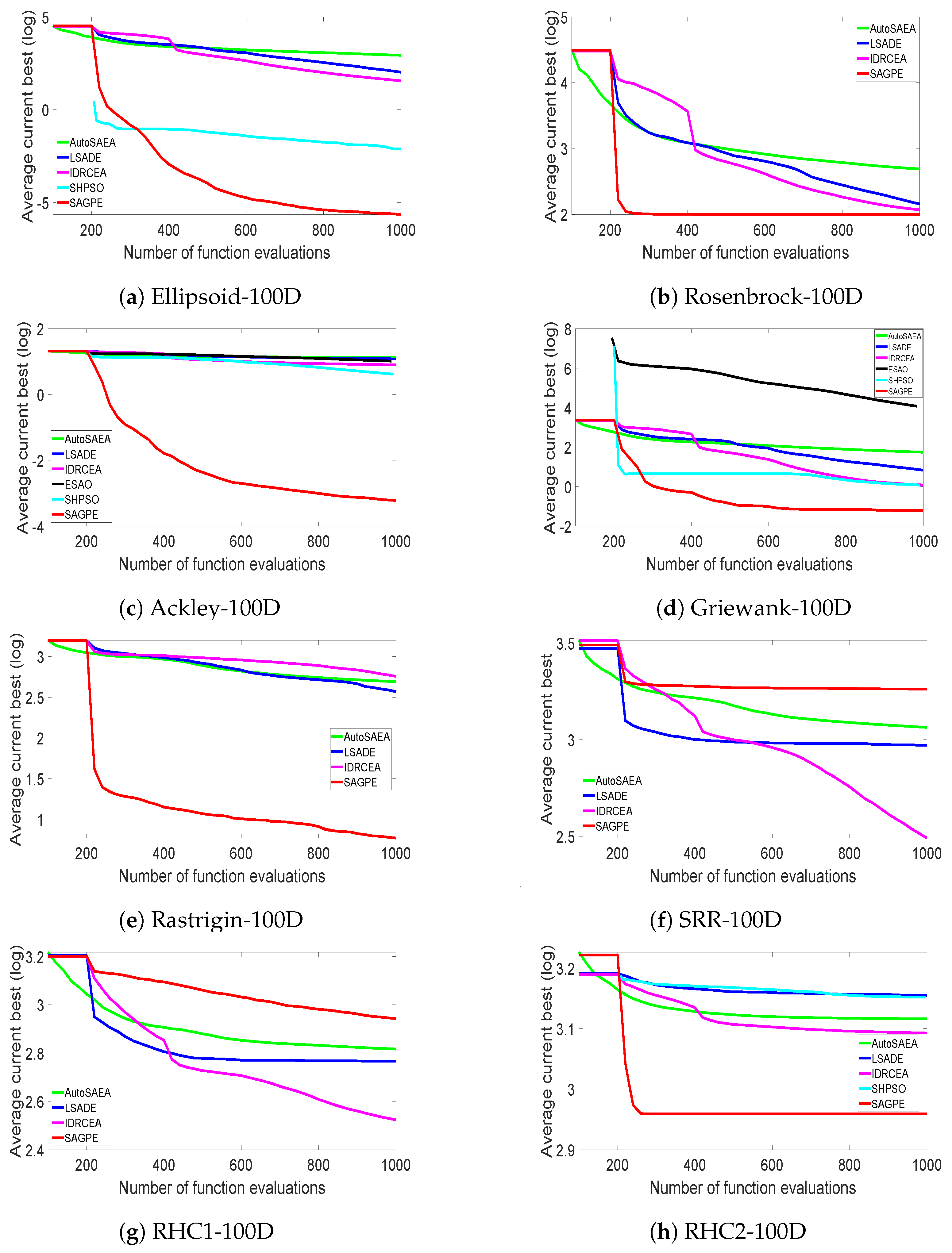
4.3. Experimental Results on 30D, 50D, and 100D Benchmark Functions

To examine the performance of SAGPE, it was tested on commonly used benchmark functions and compared to the five SAEAs mentioned above at 30D, 50D, and 100D, respectively. For all the algorithms, the average values of fitness and corresponding standard deviations are shown in Table 2. For ease of observation, the best value for each test function is recorded using black bold font in the table. As can be seen from Table 2, the overall optimization performance of SAGPE is better than the other five compared algorithms. SAGPE has better average values than the other five algorithms in 14 of the 24 problems tested. Table 2 shows that SAGPE has the best optimization results on 30D for Ellipsoid, Ackley, and Rastrigin; on 50D for Ellipsoid, Ackley, Griewank, Rastrigin, and RHC2; and on 100D for Ellipsoid, Rosenbrock, Ackley, Griewank, Rastrigin, and RHC2. As the dimensionality increased, the number of benchmark functions on which SAGPE outperformed the other five algorithms increased.
SAGPE outperformed IDRCEA in 15 of 24 problems. IDRCEA generates offspring by IDS and uses RCP to select promising individuals for true functional evaluate. Compensating for the shortcomings of regression models that easily lead to population search stagnation in complex landscapes by using categorical models allows IDECEA to have superior performance on complicated multimodal problems such as SRR and RHC1. Comparatively speaking, the advantages of SAGPE are reflected in solving unimodal and multimodal problems. For the complicated multimodal problems, EGM(1,1) may not be able to accurately capture the population update trend during the search process. It is noteworthy that SAGPE achieved the optimal average value on both 50D and 100D of the complicated multimodal function RHC2. The reason may be that RHC2 is a complicated multimodal function with a narrow basin, and EGM(1,1) can accurately capture the update trend of the population in the narrow basin, thus guiding the population to find a good solution efficiently. Compared to ESAO, SAGPE yielded better averages on 13 out of 18 problems. A global RBF model and a local RBF model are used alternately in both SAGPE and ESAO. As can be seen in Table 2, ESAO has superior performance in solving medium-dimensional problems. For example, Rosenbrock’s 30D and 50D both achieved better optimization results than SAGPE. This may be due to the fact that the local search of ESAO selects the local model optima for the true evaluation, which allows ESAO to find good solutions in a narrow domain. However, it is difficult to construct accurate local models in promising regions as dimensionality increases, which ultimately leads to poor optimization performance of ESAO in high-dimensional problems. The EGM(1,1) operator in GPE has the ability to predict the trend of population updates, which can synergize with the surrogate model to assist the population search. This feature allows SAGPE to guide the population search to promising areas by predicting the population update trend through EGM(1,1), even when an accurate surrogate model cannot be constructed. Compared to AutoSAEA, SAGPE has better averages on 15 out of 24 problems. AutoSAEA improves the quality of candidate individuals by automatically configuring surrogate models and prescreening strategies during optimization, and it has the average on 30D Griewank. However, the reliance on surrogates makes AutoSAEA poor at solving high-dimensional problems, although it solves low-dimensional problems well. Comparatively, the predictive search mechanism of GPE in SAGPE reduces the dependence of population search on surrogate models and does not drastically degrade optimization performance in high-dimensional problems due to the difficulty of constructing accurate surrogate models. As a result, AutoSAEA optimized Rosenbrock, Griewank, and RHC2 better than SAGPE at 30D, but not as well as SAGPE at 50D and 100D. The predictive search mechanism of GPE in SAGPE has a more powerful global search capability than traditional EAs. Although SHPSO uses a multipopulation strategy with PSO and SL-PSO working in tandem to enhance the global search capability, SAGPE outperformed SHPSO on average in 14 out of 21 problems. In addition, the inferior offspring learning strategy in SAGPE can significantly improve the search capability of the population. The average values of LSADE are mostly inferior to those of SAGPE due to its weak exploration and exploitation capabilities. Overall, the proposed SAGPE has better optimization results compared to all the above algorithms.
To evaluate the overall performance of all algorithms, Friedman’s test was used to rank the optimization performance of each algorithm on each dimension (the lower, the better). Table 3 records the results of Friedman’s statistical analysis. Table 3 shows that SAGPE has the best overall performance among the eight commonly used benchmark functions, with an average ranking of 2.39. SAGPE ranks first in the 50D and 100D cases, demonstrating its superior performance in solving high-dimensional functions. In the 30D case, SAGPE ranks third and is still competitive.
In addition to the optimization results, the convergence speed is also one of the metrics to judge the performance of an algorithm. From the convergence curves in Figure 4 show that, except for SRR and RHC1, the proposed SAGPE was faster than the other five algorithms in all dimensions of the remaining benchmark functions. This proves that SAGPE is more suitable than other algorithms for optimization with less available resources. It is worth noting from the SRR convergence curve in Figure 4 that SAGPE quickly fell into local optima in the early stages of optimization. The main reason may be the existence of a large number of local minima in the SRR and the large discrepancy between the function values of the locally optimal solution and those of the surrounding region. In GPE, each individual in the population searches in its promising direction as predicted by EGM(1,1). Although the feature that each individual in the population has its unique search direction enhances the global search capability of the algorithm, it is easy to make the individuals in the population scatter in the local optimal region for searching when solving functions with a large number of local minima such as SRR. At the same time, the SRR function has the characteristic that the function value of the local optimal solution differs greatly from the function value of the surrounding area, which makes it difficult for the GPE to jump out of the local search area using the random perturbation operator within the limited computational resources. Therefore, although SAGPE has superior performance on unimodal and multimodal problems, its optimization performance on complex multimodal problems needs to be strengthened.

4.4. Effects of Inferior Offspring Learning Strategy

To analyze the impact of the proposed inferior offspring learning strategy on the performance of the optimization algorithm, the proposed SAGPE was compared with SAGPE-W without the inferior offspring learning strategy on eight commonly used benchmark functions. The optimization results of the two methods after 30 independent runs are shown in Table 4. From Table 4, it can be seen that SAGPE yielded better optimization results than SAGPE-W on most of the benchmark problems, which proves that the inferior offspring learning strategy can effectively enhance the performance of SAGPE.
In addition, the contributions of global and local search of the two algorithms to the search for good solutions were investigated. Table 4 records the average number of true function evaluations (NFEs) and true improvements (NTIs) over all benchmark functions for the two search phases of SAGPE and SAGPE-W. It can be seen that the NFE of the global search for both SAGPE and SAGPE-W was always higher than the NFE of the local search, but this difference is not very large. To some extent, this phenomenon is a reflection of the fact that both SAGPE and SAGPE-W are well balanced between the exploration capability of the global model and the development capability of the local model. For SAGPE-W, except for F1-50D, the NTI in the global search was always greater than the NTI in the local search. This is reasonable because both global and local searches select the offspring with the best predicted fitness values for true evaluation. The local model focuses on accurate prediction in a small area without covering the entire search space. The local model will not be able to provide accurate prediction results for the offspring if the offspring is not within the accurate prediction region of the local model, which affects the search efficiency. It is worth noting that both the NFE and NTI of the global search were higher in SAGPE than in SAGPE-W. This may be due to the fact that the inferior offspring learning strategy in the global search of SAGPE improves the population’s ability to search for good solutions, and the NFE improves with increasing NTI. This presents further evidence for the effectiveness of the inferior offspring learning strategy.

4.5. Comparison of Different EAs

To test the superiority of GPE in the framework of SAEAs, this paper compared GPE with traditional EAs that search by mutation and crossover. The most commonly used EAs in SAEAs are DE and PSO [9]. Therefore, DE and PSO were selected as the comparison EAs. In the following, the reproduction operations of the DE and the PSO used for the comparison are described.
Suppose there is a population X = ( x 1 , x 2 , , x n ) , where each x represents a D-dimensional vector. The DE generates the mutation vector v by the following mutation operation:
v i = x i 1 + F ( x i 2 x i 3 ) , i = 1 , 2 , , n .
Therein, subscripts i 1 , i 2 , and i 3 are randomly generated integers in [1, n], which differ from each other, and none is equal to i. F is a scaling factor in the range [0, 1]. Then, the reproduction operation is completed by generating a new x i by combining x i and v i by following the crossover operator:
x i j = v i j , if j = j rand or r i j C r x i j , otherwise , i = 1 , 2 , , n .
Therein, j = j rand is a random integer between [1, D] and r i j = r a n d ( 0 , 1 ) . C r is the crossover probability in the range [0, 1].
For PSO, the reproduction operation is performed using the following formulas:
v i = v i + c 1 × r a n d ( p b e s t i x i ) + c 2 × r a n d ( g b e s t x i ) , i = 1 , 2 , , n .
x i = x i + v i , i = 1 , 2 , , n .
In the above two formulas, v i is the individual’s velocity, x i is the individual’s current position, and c 1 and c 2 are learning factors. p b e s t i is the historical optimal position of the ith individual, and g b e s t is the global optimal position.
To test the fairness of the test, this paper simply replaced the GPE in the above SAGPE-W with DE and PSO, respectively, and the rest of the conditions remained unchanged. GPE, DE, and PSO were tested as basic algorithms in the same SAEAs framework on the CEC2014 [34] function set of 50D, respectively. In DE, F was set to 0.6, and C r was set to 0.8. c 1 and c 2 were both set to 2 in PSO. Table 5 shows the average results of 30 independent runs. The results of the Wilcoxon rank sum test show that GPE achieved better optimization results than DE for 18 out of 30 test functions and similar results for 4 test functions. GPE outperformed PSO in 21 of the tested functions and showed similar results on 4 of the tested functions. The above results show that GPE, which searches through population prediction information, performs better in the SAEAs framework than DE and PSO, which search through the interaction of information from current or historical individuals.

4.6. Application on the Speed Reducer Design

In this subsection, the proposed SAGPE was applied to solve the speed reducer design problem to test its performance in dealing with real engineering problems. The problem consists of seven variables, where x 1 is the width of the tooth surface, x 2 is the module of the tooth, x 3 is the number of teeth on the pinion, x 4 is the length of the first shaft between the bearings, x 5 is the length of the second shaft between the bearings, x 6 is the diameter of the first shaft, and x 7 is the diameter of the second shaft. The design goal is to minimize the weight of the speed reducer. The mathematical model of the problem is described as follows:
f ( x 1 , x 2 , x 3 , x 4 , x 5 , x 6 , x 7 ) =   0.7854 x 1 x 2 2 3.3333 x 3 2 + 14.9334 x 3 43.0934   1.508 x 1 x 6 2 + x 7 2 + 7.4777 x 6 3 + x 7 3 +   0.7854 x 4 x 6 2 + x 5 x 7 2 ,
where 2.6 ≤ x 1 ≤ 3.6, 0.7 ≤ x 2 ≤ 0.8, 17 ≤ x 3 ≤ 28, 7.3 ≤ x 4 ≤ 8.3, 7.3 ≤ x 5 ≤ 8.3, 2.9 ≤ x 6 ≤ 3.9, and 5.0 ≤ x 7 ≤ 5.5.
Table 6 records the experimental results obtained after 30 independent runs using SAGPE and the compared results with those previously reported by Pan et al. [22]. From the statistical results in Table 6, it can be seen that the mean values and worst values obtained by SAGPE are superior to the other five methods. The best results and standard deviations obtained by SAGPE are competitive with the other algorithms. It can be seen that the application of the proposed SAGPE to the speed reducer design problem is effective and proves the practical application value of SAGPE.

5. Conclusions and Future Work

A surrogate-assisted gray prediction evolution algorithm (SAGPE) which can be used to solve EOPs was proposed in this article. The algorithm exploits the predictive power of the even gray model (EGM(1,1)) operator in the gray prediction evolution algorithm (GPE) to effectively balance the speed and effectiveness of optimization. In addition, an inferior offspring learning strategy is included in the global search phase to enhance the exploitation of population information. The performance of SAGPE was validated by comparing it with five state-of-the-art SAEAs on 30D, 50D, and 100D using eight benchmark functions. The superiority of SAGPE in solving EOPs was confirmed by the experimental results. The optimization performance of GPE was compared with that of classical DE and PSO with the same surrogate model and prescreening strategy through extended experiments.
The preliminary experimental results indicate that the search by the predictive information of the population has superiority in the optimization framework of SAEAs. The core of the superior performance of the proposed algorithm is the predictive power of the EGM(1,1). Therefore, it can be considered to further improve the performance of the algorithm by increasing the predictive ability of the EGM(1,1), such as increasing the number of data sequences. On this basis, adaptive selection of the number of data sequences is also a promising direction for improvement. In addition, it is also significant to combine GPE with other EAs that have strong exploitation capabilities to solve complicated multimodal problems.

Author Contributions

Conceptualization, Q.Z.; Methodology, X.H.; Software, X.H.; Validation, X.H.; Formal analysis, H.L. and Q.S.; Data curation, X.H.; Writing—original draft, X.H.; Writing—review & editing, X.H.; Visualization, X.H.; Supervision, H.L., Q.Z. and Q.S.; Project administration, H.L. and Q.Z. All authors have read and agreed to the published version of the manuscript.

Funding

This research received no external funding.

Data Availability Statement

The original contributions presented in this study are included in the article. Further inquiries can be directed to the corresponding author.

Conflicts of Interest

The authors declare no conflicts of interest.

References

  1. Xiang, X.; Su, Q.; Huang, G.; Hu, Z. A simplified non-equidistant grey prediction evolution algorithm for global optimization. Appl. Soft Comput. 2022, 125, 109081. [Google Scholar] [CrossRef]
  2. Zhu, H.; Shi, L.; Hu, Z.; Su, Q. A multi-surrogate multi-tasking genetic algorithm with an adaptive training sample selection strategy for expensive optimization problems. Eng. Appl. Artif. Intell. 2024, 130, 107684. [Google Scholar] [CrossRef]
  3. Jin, Y.; Wang, H.; Chugh, T.; Guo, D.; Miettinen, K. Data-driven evolutionary optimization: An overview and case studies. IEEE Trans. Evol. Comput. 2018, 23, 442–458. [Google Scholar] [CrossRef]
  4. Zhen, H.; Gong, W.; Wang, L.; Ming, F.; Liao, Z. Two-Stage Data-Driven Evolutionary Optimization for High-Dimensional Expensive Problems. IEEE Trans. Cybern. 2023, 53, 2368–2379. [Google Scholar] [CrossRef]
  5. Pan, J.S.; Liu, N.; Chu, S.C.; Lai, T. An efficient surrogate-assisted hybrid optimization algorithm for expensive optimization problems. Inf. Sci. 2021, 561, 304–325. [Google Scholar] [CrossRef]
  6. Hardy, R.L. Multiquadric equations of topography and other irregular surfaces. J. Geophys. Res. 1971, 76, 1905–1915. [Google Scholar] [CrossRef]
  7. Liu, B.; Zhang, Q.; Gielen, G.G. A Gaussian process surrogate model assisted evolutionary algorithm for medium scale expensive optimization problems. IEEE Trans. Evol. Comput. 2013, 18, 180–192. [Google Scholar] [CrossRef]
  8. Herrera, M.; Guglielmetti, A.; Xiao, M.; Filomeno Coelho, R. Metamodel-assisted optimization based on multiple kernel regression for mixed variables. Struct. Multidiscip. Optim. 2014, 49, 979–991. [Google Scholar] [CrossRef]
  9. Huang, K.; Zhen, H.; Gong, W.; Wang, R.; Bian, W. Surrogate-assisted evolutionary sampling particle swarm optimization for high-dimensional expensive optimization. Neural Comput. Appl. 2023, 1–17. [Google Scholar] [CrossRef]
  10. Tian, J.; Tan, Y.; Zeng, J.; Sun, C.; Jin, Y. Multiobjective infill criterion driven Gaussian process-assisted particle swarm optimization of high-dimensional expensive problems. IEEE Trans. Evol. Comput. 2018, 23, 459–472. [Google Scholar] [CrossRef]
  11. Xie, L.; Li, G.; Wang, Z.; Cui, L.; Gong, M. Surrogate-Assisted Evolutionary Algorithm with Model and Infill Criterion Auto-Configuration. IEEE Trans. Evol. Comput. 2023, 28, 1114–1126. [Google Scholar] [CrossRef]
  12. Nguyen, B.H.; Xue, B.; Zhang, M. A constrained competitive swarm optimizer with an SVM-based surrogate model for feature selection. IEEE Trans. Evol. Comput. 2022, 28, 2–16. [Google Scholar] [CrossRef]
  13. Dong, H.; Dong, Z. Surrogate-assisted grey wolf optimization for high-dimensional, computationally expensive black-box problems. Swarm Evol. Comput. 2020, 57, 100713. [Google Scholar] [CrossRef]
  14. Li, G.; Zhang, Q.; Lin, Q.; Gao, W. A three-level radial basis function method for expensive optimization. IEEE Trans. Cybern. 2021, 52, 5720–5731. [Google Scholar] [CrossRef]
  15. Li, G.; Wang, Z.; Gong, M. Expensive optimization via surrogate-assisted and model-free evolutionary optimization. IEEE Trans. Syst. Man. Cybern. Syst. 2022, 53, 2758–2769. [Google Scholar] [CrossRef]
  16. Wang, H.; Jin, Y.; Doherty, J. Committee-based active learning for surrogate-assisted particle swarm optimization of expensive problems. IEEE Trans. Cybern. 2017, 47, 2664–2677. [Google Scholar] [CrossRef]
  17. Di Nuovo, A.G.; Ascia, G.; Catania, V. A study on evolutionary multi-objective optimization with fuzzy approximation for computational expensive problems. In Proceedings of the Parallel Problem Solving from Nature-PPSN XII: 12th International Conference, Taormina, Italy, 1–5 September 2012; Springer: Berlin/Heidelberg, Germany, 2012. Part II. pp. 102–111. [Google Scholar] [CrossRef]
  18. Li, F.; Shen, W.; Cai, X.; Gao, L.; Wang, G.G. A fast surrogate-assisted particle swarm optimization algorithm for computationally expensive problems. Appl. Soft Comput. 2020, 92, 106303. [Google Scholar] [CrossRef]
  19. Ong, Y.S.; Nair, P.B.; Keane, A.J. Evolutionary optimization of computationally expensive problems via surrogate modeling. AIAA J. 2003, 41, 687–696. [Google Scholar] [CrossRef]
  20. Li, G.; Zhang, Q. Multiple penalties and multiple local surrogates for expensive constrained optimization. IEEE Trans. Evol. Comput. 2021, 25, 769–778. [Google Scholar] [CrossRef]
  21. Wang, X.; Wang, G.G.; Song, B.; Wang, P.; Wang, Y. A novel evolutionary sampling assisted optimization method for high-dimensional expensive problems. IEEE Trans. Evol. Comput. 2019, 23, 815–827. [Google Scholar] [CrossRef]
  22. Pan, J.S.; Liang, Q.; Chu, S.C.; Tseng, K.K.; Watada, J. A multi-strategy surrogate-assisted competitive swarm optimizer for expensive optimization problems. Appl. Soft Comput. 2023, 147, 110733. [Google Scholar] [CrossRef]
  23. Guo, Z.; Zhang, Z.; Chen, Y.; Ma, G.; Song, L.; Li, J.; Feng, Z. An efficient surrogate-assisted differential evolution algorithm for turbomachinery cascades optimization with more than 100 variables. Aerosp. Sci. Technol. 2023, 142, 108675. [Google Scholar] [CrossRef]
  24. Zhang, J.; Li, M.; Yue, X.; Wang, X.; Shi, M. A hierarchical surrogate assisted optimization algorithm using teaching-learning-based optimization and differential evolution for high-dimensional expensive problems. Appl. Soft Comput. 2024, 152, 111212. [Google Scholar] [CrossRef]
  25. Meng, Z.; Yang, C. Hip-DE: Historical population based mutation strategy in differential evolution with parameter adaptive mechanism. Inf. Sci. 2021, 562, 44–77. [Google Scholar] [CrossRef]
  26. Hu, Z.; Xu, X.; Su, Q.; Zhu, H.; Guo, J. Grey prediction evolution algorithm for global optimization. Appl. Math. Model. 2020, 79, 145–160. [Google Scholar] [CrossRef]
  27. Li, W.; Su, Q.; Hu, Z. A grey prediction evolutionary algorithm with a surrogate model based on quadratic interpolation. Expert Syst. Appl. 2024, 236, 121261. [Google Scholar] [CrossRef]
  28. Jin, R.; Chen, W.; Simpson, T.W. Comparative studies of metamodelling techniques under multiple modelling criteria. Struct. Multidiscip. Optim. 2001, 23, 1–13. [Google Scholar] [CrossRef]
  29. Díaz-Manríquez, A.; Toscano, G.; Coello Coello, C.A. Comparison of metamodeling techniques in evolutionary algorithms. Soft Comput. 2017, 21, 5647–5663. [Google Scholar] [CrossRef]
  30. Stein, M. Large sample properties of simulations using Latin hypercube sampling. Technometrics 1987, 29, 143–151. [Google Scholar] [CrossRef]
  31. Kuudela, J.; Matousek, R. Combining Lipschitz and RBF surrogate models for high-dimensional computationally expensive problems. Inf. Sci. 2023, 619, 457–477. [Google Scholar] [CrossRef]
  32. Li, G.; Xie, L.; Wang, Z.; Wang, H.; Gong, M. Evolutionary algorithm with individual-distribution search strategy and regression-classification surrogates for expensive optimization. Inf. Sci. 2023, 634, 423–442. [Google Scholar] [CrossRef]
  33. Yu, H.; Tan, Y.; Zeng, J.; Sun, C.; Jin, Y. Surrogate-assisted hierarchical particle swarm optimization. Inf. Sci. 2018, 454, 59–72. [Google Scholar] [CrossRef]
  34. Liang, J.J.; Qu, B.Y.; Suganthan, P.N. Problem definitions and evaluation criteria for the CEC 2014 special session and competition on single objective real-parameter numerical optimization. Comput. Intell. Lab. Zhengzhou Univ. Zhengzhou China Tech. Rep. Nanyang Technol. Univ. Singap. 2013, 635, 2014. [Google Scholar]
Figure 1. Framework of the proposed SAGPE.
Mathematics 13 01007 g001
Figure 2. Results for (a) Ellipsoid, (b) Ackley, and (c) SRR functions for different values of η .
Mathematics 13 01007 g002
Figure 3. Results for different population sizes for (a) Ellipsoid, (b) Ackley, and (c) SRR functions.
Mathematics 13 01007 g003
Figure 4. Convergence curves of AutoSAEA, LSADE, IDRCEA, EASO, SHPSO, and SAGPE on 100D functions.
Mathematics 13 01007 g004
Table 1. Characteristics of eight benchmark functions.
FunctionDimensionOptimunProperty
F1Ellipsoid30 50 1000Unimodal
F2Rosenbrock30 50 1000Multimodal with narrow valley
F3Ackley30 50 1000Multimodal
F4Griewank30 50 1000Multimodal
F5Rastrigin30 50 1000Multimodal
F6Shifted Rotated Rastrigin (SRR)30 50 100 330 Very complicated multimodal
F7Rotated Hybrid Composition function (RHC1)30 50 100120Very complicated multimodal
F8Rotated Hybrid Composition function (RHC2)30 50 10010Very complicated multimodal with a narrow basin
Table 2. Comparison of results of five SAEAs on 30D, 50D, and 100D functions.
Algorithm AutoSAEA (Mean/Std)LSADE (Mean/Std)IDRCEA (Mean/Std)ESAO (Mean/Std)SHPSO (Mean/Std)SAGPE (Mean/Std)
FunD
F1302.01 × 10 5 /2.03 × 10 5 (+)1.49 × 10 2 /2.27 × 10 2 (+)4.48 × 10 4 /4.24 × 10 4 (+)2.75 × 10 2 /6.96 × 10 2 (+)2.12 × 10 1 /1.52 × 10 1 (+)9.40 × 10 8 /5.18 × 10 8
F2302.58 × 10 1 /1.02 × 10 0 (−)2.69 × 10 1 /1.04 × 10 0 (−)2.64 × 10 1 /5.56 × 10 1 (−)2.50 × 10 1 /1.57 × 10 0 (−)2.86 × 10 1 /4.04 × 10 1 (+)2.73 × 10 1 /1.89 × 10 1
F3301.90 × 10 1 /4.39 × 10 1 (+)1.57 × 10 0 /1.07 × 10 0 (+)1.25 × 10 0 /7.20 × 10 1 (+)2.52 × 10 0 /8.40 × 10 1 (+)1.44 × 10 0 /7.74 × 10 1 (+)7.12 × 10 5 /1.46 × 10 5
F4301.40 × 10 3 /3.10 × 10 3 (−)5.45 × 10 2 /2.58 × 10 2 (+)4.38 × 10 3 /6.30 × 10 3 (−)9.53 × 10 1 /5.04 × 10 2 (+)9.21 × 10 1 /8.81 × 10 2 (+)2.55 × 10 2 /4.79 × 10 2
F5304.27 × 10 1 /2.15 × 10 1 (+)8.11 × 10 1 /1.89 × 10 1 (+)3.54 × 10 1 /2.13 × 10 1 (+)NaNNaN4.67 × 10 0 /6.15 × 10 1
F630−2.55 × 10 2 /2.85 × 10 1 (−)−2.11 × 10 2 /3.75 × 10 1 (−)−2.78 × 10 2 /1.45 × 10 1 (−)6.33 × 10 0 /2.65 × 10 1 (−)−8.25 × 10 1 /2.25 × 10 1 (−)1.65 × 10 2 /4.50 × 10 1
F7303.82 × 10 2 /1.56 × 10 2 (−)4.37 × 10 2 /1.58 × 10 2 (−)3.47 × 10 2 /1.72 × 10 2 (−)NaN4.64 × 10 2 /8.51 × 10 1 (−)6.01 × 10 2 /7.54 × 10 1
F8309.34 × 10 2 /8.38 × 10 0 (−)9.63 × 10 2 /4.24 × 10 1 (+)9.50 × 10 2 /9.00 × 10 0 (+)9.32 × 10 2 /8.94 × 10 0 (−)9.40 × 10 2 /9.02 × 10 0 (−)9.48 × 10 2 /7.24 × 10 1
F1508.48 × 10 1 /7.79 × 10 1 (+)1.26 × 10 0 /8.75 × 10 1 (+)3.22 × 10 1 /2.69 × 10 1 (+)7.40 × 10 1 /5.55 × 10 1 (+)4.03 × 10 0 /2.06 × 10 0 (+)8.72 × 10 7 /3.76 × 10 7
F2504.95 × 10 1 /9.73 × 10 0 (+)4.91 × 10 1 /7.62 × 10 0 (+)4.75 × 10 1 /7.58 × 10 1 (−)4.74 × 10 1 /1.71 × 10 0 (−)5.08 × 10 1 /3.03 × 10 0 (+)4.81 × 10 1 /4.75 × 10 1
F3502.31 × 10 0 /6.78 × 10 1 (+)7.47 × 10 0 /3.22 × 10 0 (+)3.78 × 10 0 /6.46 × 10 1 (+)1.43 × 10 0 /2.49 × 10 1 (+)1.84 × 10 0 /5.64 × 10 1 (+)1.51 × 10 4 /4.56 × 10 5
F4502.22 × 10 1 /7.08 × 10 2 (+)8.11 × 10 1 /1.36 × 10 1 (+)1.36 × 10 1 /6.53 × 10 2 (+)9.40 × 10 1 /4.21 × 10 2 (+)9.45 × 10 1 /6.14 × 10 2 (+)6.60 × 10 3 /3.60 × 10 2
F5501.01 × 10 2 /2.73 × 10 1 (+)1.54 × 10 2 /3.51 × 10 1 (+)8.11 × 10 1 /4.94 × 10 1 (+)NanNaN1.67 × 10 0 /3.85 × 10 0
F650−1.48 × 10 2 /4.27 × 10 1 (−)−1.03 × 10 2 /5.40 × 10 1 (−)−2.19 × 10 2 /3.08 × 10 1 (−)1.98 × 10 2 /4.58 × 10 1 (−)1.34 × 10 2 /3.25 × 10 1 (−)7.06 × 10 2 /8.12 × 10 1
F7503.03 × 10 2 /8.59 × 10 1 (−)3.64 × 10 2 /1.07 × 10 2 (−)2.75 × 10 2 /1.05 × 10 2 (−)NaN4.74 × 10 2 /4.20 × 10 1 (−)7.33 × 10 2 /9.77 × 10 1
F8501.04 × 10 3 /4.38 × 10 1 (+)1.04 × 10 3 /6.95 × 10 1 (+)1.03 × 10 3 /2.08 × 10 1 (+)9.57 × 10 2 /3.71 × 10 1 (+)9.97 × 10 2 /2.21 × 10 1 (+)9.10 × 10 2 /4.41 × 10 6
F11008.69 × 10 2 /2.09 × 10 2 (+)1.06 × 10 2 /2.68 × 10 1 (+)3.66 × 10 1 /1.37 × 10 1 (+)1.28 × 10 3 /1.34 × 10 2 (+)7.61 × 10 1 /2.14 × 10 1 (+)9.29 × 10 5 /6.83 × 10 5
F21004.88 × 10 2 /7.86 × 10 1 (+)1.42 × 10 2 /1.88 × 10 1 (+)1.17 × 10 2 /1.14 × 10 1 (+)5.78 × 10 2 /4.48 × 10 1 (+)1.66 × 10 2 /2.64 × 10 1 (+)9.87 × 10 1 /1.62 × 10 1
F31001.35 × 10 1 /6.03 × 10 1 (+)1.21 × 10 1 /1.63 × 10 0 (+)7.95 × 10 0 /7.88 × 10 1 (+)1.04 × 10 1 /2.11 × 10 1 (+)4.11 × 10 0 /5.92 × 10 1 (+)6.03 × 10 4 /1.39 × 10 4
F41005.52 × 10 1 /1.46 × 10 1 (+)6.75 × 10 0 /1.49 × 10 0 (+)1.21 × 10 0 /9.80 × 10 2 (+)5.73 × 10 1 /5.84 × 10 0 (+)1.07 × 10 0 /2.05 × 10 2 (+)3.32 × 10 2 /7.27 × 10 2
F51004.92 × 10 2 /7.55 × 10 1 (+)3.71 × 10 2 /7.54 × 10 1 (+)5.72 × 10 2 /1.35 × 10 2 (+)NaNNaN6.0 × 10 0 /5.75 × 10 0
F61001.16 × 10 3 /9.96 × 10 1 (−)9.34 × 10 2 /1.02 × 10 2 (−)3.10 × 10 2 /8.42 × 10 1 (−)7.13 × 10 2 /2.65 × 10 1 (−)8.02 × 10 2 /7.23 × 10 1 (−)1.83 × 10 3 /6.99 × 10 1
F71006.55 × 10 2 /6.07 × 10 1 (−)5.84 × 10 2 /3.66 × 10 1 (−)3.34 × 10 2 /2.60 × 10 1 (−)NaN5.16 × 10 2 /3.21 × 10 1 (−)8.76 × 10 2 /1.21 × 10 2
F81001.31 × 10 3 /2.16 × 10 1 (+)1.43 × 10 3 /3.44 × 10 1 (+)1.24 × 10 3 /3.18 × 10 1 (+)1.37 × 10 3 /2.75 × 10 1 (+)1.42 × 10 3 /3.82 × 10 1 (+)9.10 × 10 2 /2.51 × 10 4
+/−/= 15/9/017/7/015/9/013/5/014/7/0NaN/NaN/NaN
Table 3. Friedman test results for all functions.
MothodsDAvg. RankOverall Rank
30D50D100D
AutoSAEA1.833.584.833.423
LSADE4.334.254.334.315
IDRCEA2.832.502.172.502
ESAO4.004.254.674.316
SHPSO4.674.423.174.084
SAGPE3.332.001.832.391
Table 4. Experimental results of SAGPE and SAGPE-W for 30D, 50D, and 100D functions.
MothodsSAGPESAGPE-W
FunGlobal Search
(NFE/NTI)
Local Search
(NFE/NTI)
Mean/StdGlobal Search
(NFE/NTI)
Local Search
(NFE/NTI)
Mean/Std
F1-30D472.9/27.4467.6/22.19.40 × 10 8 /5.18 × 10 8 473.1/23.9467.5/18.48.88 × 10 8 /4.60 × 10 8
F2-30D486.6/48.4453.9/15.82.73 × 10 1 /1.89 × 10 1 474.6/2.73 × 10 1 465.7/18.42.78 × 10 1 /3.48 × 10 1
F3-30D470.2/17.9470.3/18.17.12 × 10 5 /1.46 × 10 5 468.6/13.7471.9/16.97.67 × 10 5 /1.63 × 10 5
F4-30D475.6/22.6464.9/11.82.55 × 10 2 /4.79 × 10 2 472.9/16.8467.5/11.41.79 × 10 2 /6.09 × 10 2
F5-30D475.2/24.9465.4/15.14.67 × 10 0 /6.15 × 10 0 471.4/17.7468.1/15.53.30 × 10 0 /5.52 × 10 0
F6-30D474.3/9.00466.4/1.171.65 × 10 2 /4.50 × 10 0 471.7/6.30468.8/3.472.13 × 10 2 /4.88 × 10 1
F7-30D487.6/37.3452.8/2.436.01 × 10 2 /7.54 × 10 1 475.4/25.3465.3/15.36.82 × 10 2 /6.74 × 10 1
F8-30D475.6/23.3464.9/12.79.48 × 10 2 /7.24 × 10 1 471.0/16.2469.4/14.69.14 × 10 2 /2.27 × 10 1
F1-50D451.6/24.4448.7/21.57.69 × 10 7 /3.78 × 10 7 450.1/18.7450.5/19.08.74 × 10 7 /4.59 × 10 7
F2-50D464.7/45.1435.7/16.14.76 × 10 1 /4.10 × 10 1 455.8/31.7444.8/20.74.81 × 10 1 /3.12 × 10 1
F3-50D451.2/19.8449.5/18.11.39 × 10 4 /3.37 × 10 5 450.7/16.9449.8/15.91.43 × 10 4 /4.05 × 10 5
F4-50D459.3/24.6441.1/6.475.24 × 10 2 /7.14 × 10 2 456.7/19.6443.8/4.735.30 × 10 2 /2.91 × 10 2
F5-50D456.9/20.8443.7/7.631.99 × 10 0 /1.97 × 10 0 453.6/15.4446.9/8.778.57 × 10 1 /7.22 × 10 1
F6-50D455.2/11.0445.3/1.176.48 × 10 2 /7.62 × 10 1 452.4/8.40448.2/4.207.02 × 10 2 /8.86 × 10 1
F7-50D466.0/33.3434.7/1.936.44 × 10 2 /5.23 × 10 1 453.1/16.8447.5/11.37.17 × 10 2 /8.98 × 10 1
F8-50D452.6/23.6447.7/18.79.10 × 10 2 /2.92 × 10 6 451.1/18.7449.3/16.99.10 × 10 2 /4.28 × 10 6
F1-100D402.2/16.9398.2/12.99.29 × 10 5 /6.83 × 10 5 402.4/16.0398.0/11.61.55 × 10 4 /9.69 × 10 5
F2-100D405.8/23.3394.7/12.19.87 × 10 1 /1.62 × 10 1 401.7/15.3398.7/12.39.88 × 10 1 /6.86 × 10 2
F3-100D405.8/24.3394.7/13.26.03 × 10 4 /1.39 × 10 4 404.5/18.7396.1/10.46.45 × 10 4 /1.67 × 10 4
F4-100D410.7/27.7389.8/6.803.32 × 10 2 /7.27 × 10 2 408.0/21.0392.5/5.531.79 × 10 4 /3.41 × 10 4
F5-100D404.9/14.4395.6/5.126.01 × 10 0 /5.75 × 10 0 405.0/14.3395.5/4.832.60 × 10 1 /8.57 × 10 0
F6-100D403.0/7.07397.6/1.701.83 × 10 3 /6.99 × 10 1 401.2/5.27399.4/3.501.90 × 10 3 /4.89 × 10 1
F7-100D411.3/24.2389.1/1.978.76 × 10 2 /1.21 × 10 2 401.6/11.9398.9/9.179.83 × 10 2 /1.58 × 10 2
F8-100D406.0/23.3394.7/11.99.10 × 10 2 /2.51 × 10 4 4.3.1/16.5397.5/10.99.10 × 10 2 /3.00 × 10 4
Table 5. Experimental results of different surrogate-assisted EAs in the 50-D CEC2014 test set.
Algorithm GPE (Mean/Std)DE (Mean/Std)PSO (Mean/Std)
FunD
F1507.48 × 10 8 /1.48 × 10 8 1.76 × 10 9 /3.14 × 10 8 (+)4.76 × 10 9 /1.25 × 10 9 (+)
F2502.34 × 10 10 /5.57 × 10 9 5.10 × 10 8 /6.67 × 10 8 (−)1.12 × 10 11 /9.58 × 10 9 (+)
F3501.66 × 10 5 /2.45 × 10 4 3.46 × 10 5 /5.45 × 10 4 (+)1.45 × 10 5 /2.49 × 10 4 (−)
F4503.60 × 10 3 /1.11 × 10 3 5.40 × 10 3 /2.16 × 10 3 (+)2.07 × 10 4 /1.38 × 10 3 (+)
F5505.21 × 10 2 /6.46 × 10 2 5.21 × 10 2 /4.77 × 10 2 (=)5.21 × 10 2 /5.46 × 10 2 (=)
F6506.70 × 10 2 /2.16 × 10 0 6.80 × 10 2 /1.73 × 10 0 (+)6.69 × 10 2 /3.10 × 10 0 (−)
F7509.97 × 10 2 /8.04 × 10 1 8.40 × 10 2 /1.10 × 10 2 (−)1.77 × 10 3 /7.43 × 10 1 (+)
F8501.47 × 10 3 /3.94 × 10 1 1.37 × 10 3 /3.19 × 10 1 (−)1.49 × 10 3 /3.89 × 10 1 (+)
F9501.58 × 10 3 /3.45 × 10 1 1.55 × 10 3 /3.93 × 10 1 (−)1.60 × 10 3 /4.69 × 10 1 (+)
F10501.58 × 10 4 /6.68 × 10 2 1.62 × 10 4 /5.12 × 10 2 (+)1.68 × 10 4 /9.14 × 10 2 (+)
F11501.62 × 10 4 /4.91 × 10 2 1.67 × 10 4 /4.67 × 10 2 (+)1.59 × 10 4 /7.04 × 10 2 (−)
F12501.21 × 10 3 /6.00 × 10 1 1.21 × 10 3 /5.97 × 10 1 (=)1.21 × 10 3 /7.64 × 10 1 (=)
F13501.31 × 10 3 /1.54 × 10 1 1.31 × 10 3 /7.90 × 10 1 (=)1.31 × 10 3 /2.71 × 10 1 (=)
F14501.65 × 10 3 /1.69 × 10 1 1.57 × 10 3 /3.33 × 10 1 (−)1.66 × 10 3 /2.38 × 10 1 (+)
F15508.71 × 10 5 /2.76 × 10 6 2.83 × 10 6 /1.85 × 10 6 (+)4.75 × 10 5 /8.36 × 10 4 (−)
F16501.62 × 10 3 /2.00 × 10 1 1.62 × 10 3 /1.81 × 10 1 (=)1.62 × 10 3 /2.15 × 10 1 (=)
F17501.86 × 10 8 /6.01 × 10 7 2.36 × 10 8 /8.78 × 10 7 (+)6.89 × 10 8 /2.06 × 10 8 (+)
F18501.37 × 10 9 /5.04 × 10 8 3.31 × 10 9 /8.10 × 10 8 (+)1.71 × 10 10 /8.30 × 10 8 (+)
F19502.35 × 10 3 /5.35 × 10 1 2.59 × 10 3 /1.29 × 10 2 (+)3.61 × 10 3 /3.64 × 10 1 (+)
F20502.32 × 10 5 /8.91 × 10 4 2.43 × 10 6 /1.47 × 10 6 (+)2.37 × 10 6 /1.25 × 10 7 (+)
F21504.79 × 10 7 /1.68 × 10 7 1.05 × 10 8 /2.84 × 10 7 (+)4.22 × 10 7 /3.89 × 10 7 (−)
F22502.37 × 10 4 /1.47 × 10 4 6.13 × 10 3 /6.57 × 10 2 (−)4.16 × 10 5 /2.41 × 10 5 (+)
F23502.53 × 10 3 /2.78 × 10 1 3.67 × 10 3 /1.64 × 10 2 (+)3.48 × 10 3 /2.91 × 10 1 (+)
F24502.60 × 10 3 /1.43 × 10 0 3.00 × 10 3 /2.95 × 10 1 (+)2.73 × 10 3 /7.86 × 10 0 (+)
F25502.70 × 10 3 /8.92 × 10 2 2.97 × 10 3 /4.22 × 10 1 (+)2.76 × 10 3 /7.40 × 10 0 (+)
F26502.77 × 10 3 /2.53 × 10 1 2.93 × 10 3 /1.18 × 10 1 (+)2.81 × 10 3 /1.71 × 10 1 (+)
F27505.06 × 10 3 /5.65 × 10 1 5.01 × 10 3 /5.12 × 10 1 (−)6.02 × 10 3 /4.32 × 10 2 (+)
F28507.39 × 10 3 /1.65 × 10 3 1.12 × 10 4 /1.27 × 10 3 (+)2.00 × 10 4 /1.34 × 10 3 (+)
F29504.05 × 10 3 /3.43 × 10 3 5.94 × 10 8 /2.14 × 10 8 (+)2.22 × 10 9 /4.11 × 10 8 (+)
F30501.10 × 10 5 /4.65 × 10 5 6.50 × 10 6 /2.20 × 10 6 (+)5.65 × 10 7 /1.63 × 10 7 (+)
+/−/= NaN/NaN/NaN18/8/421/5/4
Table 6. Comparison of the experimental results of the speed reducer design.
AlgorithmsBestMeanWorstStd
SACSO2.2440347 × 10 3 2.5049590 × 10 3 2.3863303 × 10 3 8.7915776 × 10 1
SA-QUATRE2.3946554 × 10 3 2.3946554 × 10 3 2.3946554 × 10 3 7.7292187 × 10 13
IKAEA2.3946554 × 10 3 2.4840309 × 10 3 2.4215750 × 10 3 2.1957428 × 10 3
FSAPSO2.3946554 × 10 3 2.3946555 × 10 3 2.3946554 × 10 3 2.0117613 × 10 5
SADE-AMSS2.3946554 × 10 3 2.5626630 × 10 3 2.4813014 × 10 3 8.0224357 × 10 1
SAGPE2.3524529 × 10 3 2.3524854 × 10 3 2.3525687 × 10 3 2.8563084 × 10 2
Disclaimer/Publisher’s Note: The statements, opinions and data contained in all publications are solely those of the individual author(s) and contributor(s) and not of MDPI and/or the editor(s). MDPI and/or the editor(s) disclaim responsibility for any injury to people or property resulting from any ideas, methods, instructions or products referred to in the content.

